- 1U.S. Geological Survey, Northern Rocky Mountain Science Center, Bozeman, MT, United States
- 2Department of Mathematical Sciences, Montana State University, Bozeman, MT, United States
- 3Gage Cartographics, Bozeman, MT, United States
- 4U.S. Geological Survey, Wyoming-Montana Water Science Center, Helena, MT, United States
- 5Monterey Bay Aquarium Research Institute, Moss Landing, CA, United States
Autonomous, robotic environmental (e)DNA samplers now make it possible for biological observations to match the scale and quality of abiotic measurements collected by automated sensor networks. Merging these automated data streams may allow for improved insight into biotic responses to environmental change and stressors. Here, we merged eDNA data collected by robotic samplers installed at three U.S. Geological Survey (USGS) streamgages with gridded daily weather data, and daily water quality and quantity data into a cloud-hosted database. The eDNA targets were a rare fish parasite and a more common salmonid fish. We then used computationally expedient Bayesian hierarchical occupancy models to evaluate associations between abiotic conditions and eDNA detections and to simulate how uncertainty in result interpretation changes with the frequency of autonomous robotic eDNA sample collection. We developed scripts to automate data merging, cleaning and analysis steps into a chained-step, workflow. We found that inclusion of abiotic covariates only provided improved insight for the more common salmonid fish since its DNA was more frequently detected. Rare fish parasite DNA was infrequently detected, which caused occupancy parameter estimates and covariate associations to have high uncertainty. Our simulations found that collecting samples at least once per day resulted in more detections and less parameter uncertainty than less frequent sampling. Our occupancy and simulation results together demonstrate the advantages of robotic eDNA samplers and how these samples can be combined with easy to acquire, publicly available data to foster real-time biosurveillance and forecasting.
Introduction
Timely, up-to-date information concerning harmful invasive species and pathogens is critical for minimizing negative outcomes to ecosystem and human health (Stohlgren and Schnase, 2006; Bohan et al., 2017; Cordier et al., 2020). Assimilating this information has been challenging because the abiotic and biotic processes that drive invasive species and pathogen distributions and abundances from benign to harmful levels often occur at different spatiotemporal scales (Collins et al., 2006; Gallien et al., 2010; Uden et al., 2015). These challenges make measurement, integration, and rapid analysis difficult (Michener and Jones, 2012). For example, marine harmful algal bloom alert bulletins and early warning systems require integrating information about phytoplankton, toxin concentrations within shellfish, water temperature and wind speeds, and ocean or lake circulation forecasts (e.g., Glibert et al., 2018). Automated sensor networks, such as the U.S. Geological Survey’s (USGS) streamgage network and National Oceanic and Atmospheric Administration’s (NOAA) weather station network, have made it much easier to track changing abiotic conditions with both high and broad spatiotemporal resolution (Sepulveda et al., 2015; Al-Chokhachy et al., 2017; Kovach et al., 2019), but automated, collection of comparable biological data remains a challenge (Sugai, 2020).
Environmental (e)DNA sample collection and subsequent analyses have revolutionized biosurveillance because inferences can be made about species occurrences sight-unseen (e.g., Cristescu and Hebert, 2018). More recently, autonomous robotic eDNA samplers have made it possible to make biological observations match the scale and quality of in situ physical and chemical measurements (Yamahara et al., 2019; Sepulveda et al., 2020). Autonomous robots placed within the environment can conduct high frequency (sub-daily) sampling, regardless of location, weather, or the availability of human resources. Satellite communication ports allow results to be uploaded to end-users. Hence, biological data collection at relevant scales is no longer the bottleneck.
One current challenge is rapidly integrating the high frequency data streams produced by autonomous robotic eDNA samplers with the high frequency data streams produced by automated sensor networks tracking abiotic conditions. This integration should enable timely, up-to-date information about biological hazards. Each data stream has nuances (e.g., unique attribute fields); however, the structure of eDNA data streams presents additional complications. This molecular method provides indirect inference about species presence, so occurrence probability must be modeled (Stratton et al., 2020). For eDNA analyses, multiple samples are collected at a location and multiple replicates from each sample are analyzed for the presence of the target organism DNA. Samples taken at the location occupied by a species may not necessarily contain DNA of that target species, just like replicates may lack target DNA even if the DNA is present in the sample (Darling, 2019; Sepulveda et al., 2020). Thus, each sample and replicate may detect the organism’s DNA, if present, with some probability. Occupancy models provide a useful framework for the analysis of eDNA results (Stratton et al., 2020), in that these models account for the multiple nested levels of sampling that characterize eDNA surveys. Occupancy models also provide a useful framework for linking data streams describing abiotic conditions to those describing biological data, such as target taxa DNA (Pilliod et al., 2019; Sepulveda et al., 2019).
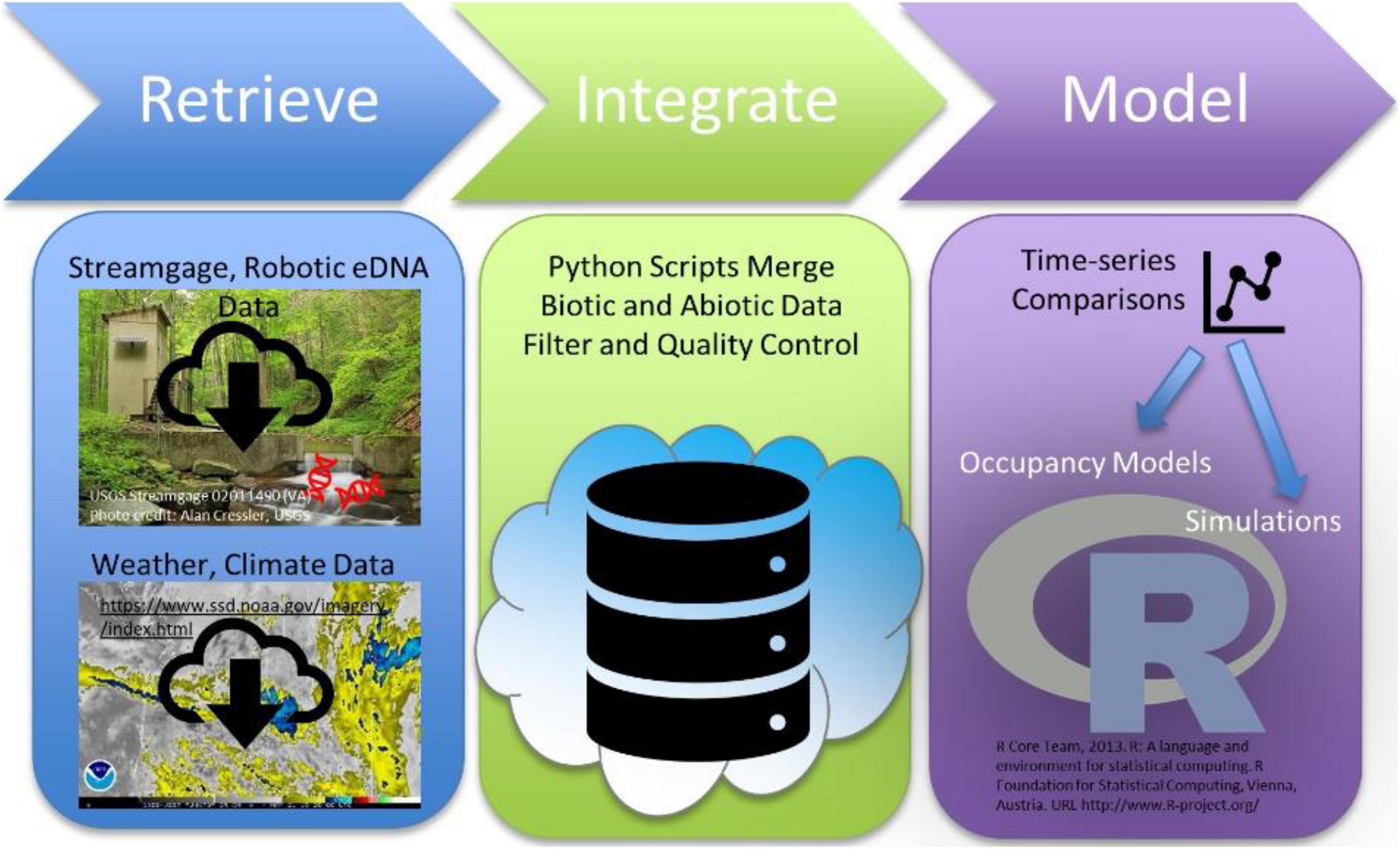
Here, we present the constituent parts of a cloud-based, data science pipeline for using Bayesian hierarchical occupancy models to analyze relationships between the high frequency data streams produced by autonomous robotic eDNA samplers and the high frequency data streams produced by automated sensor networks tracking abiotic conditions (Figure 1). To demonstrate the general applicability of this workflow, we applied it to a dataset typical of an eDNA early detection program, where target taxa DNA was rarely detected, and to a dataset typical of an eDNA monitoring program, where target taxa DNA detections were more common. To evaluate the added value of high frequency, autonomous samples, we also evaluated how uncertainty in result interpretation changes with the frequency of autonomous robotic eDNA sample collection for each dataset. Our workflow is intended to serve as a prototype for how high-throughput eDNA data can be combined with easy to acquire, publicly available data to foster real-time biosurveillance and forecasting.
Materials and Methods
eDNA Datasets
We applied the data science workflow to two datasets described in Sepulveda et al. (2020). In the first dataset used as an example of eDNA early detection programs, autonomous robotic eDNA samplers collected samples at two USGS streamgage sites in the Yellowstone River of Montana (United States): USGS 06191500 Yellowstone River at Corwin Springs MT and USGS 06192500 Yellowstone River near Livingston MT, described below as Corwin Springs and Carters Bridge, respectively (Figure 2). Robotic eDNA samplers were programmed to collect 1-L samples every 12 h, from July 24 to August 26, 2018, and every 3 h from August 27 to September 7, 2018. Samples were analyzed for DNA of the fish pathogen, Tetracapsuloides bryosalmonae, the causative agent of salmonid fish Proliferative Kidney Disease (PKD), which has resulted in large salmonid mortality events in this region and also in Europe (Hutchins et al., in press). Detections of T. bryosalmonae DNA were rare, as only 5 of 256 samples were scored as positive (Sepulveda et al., 2020).
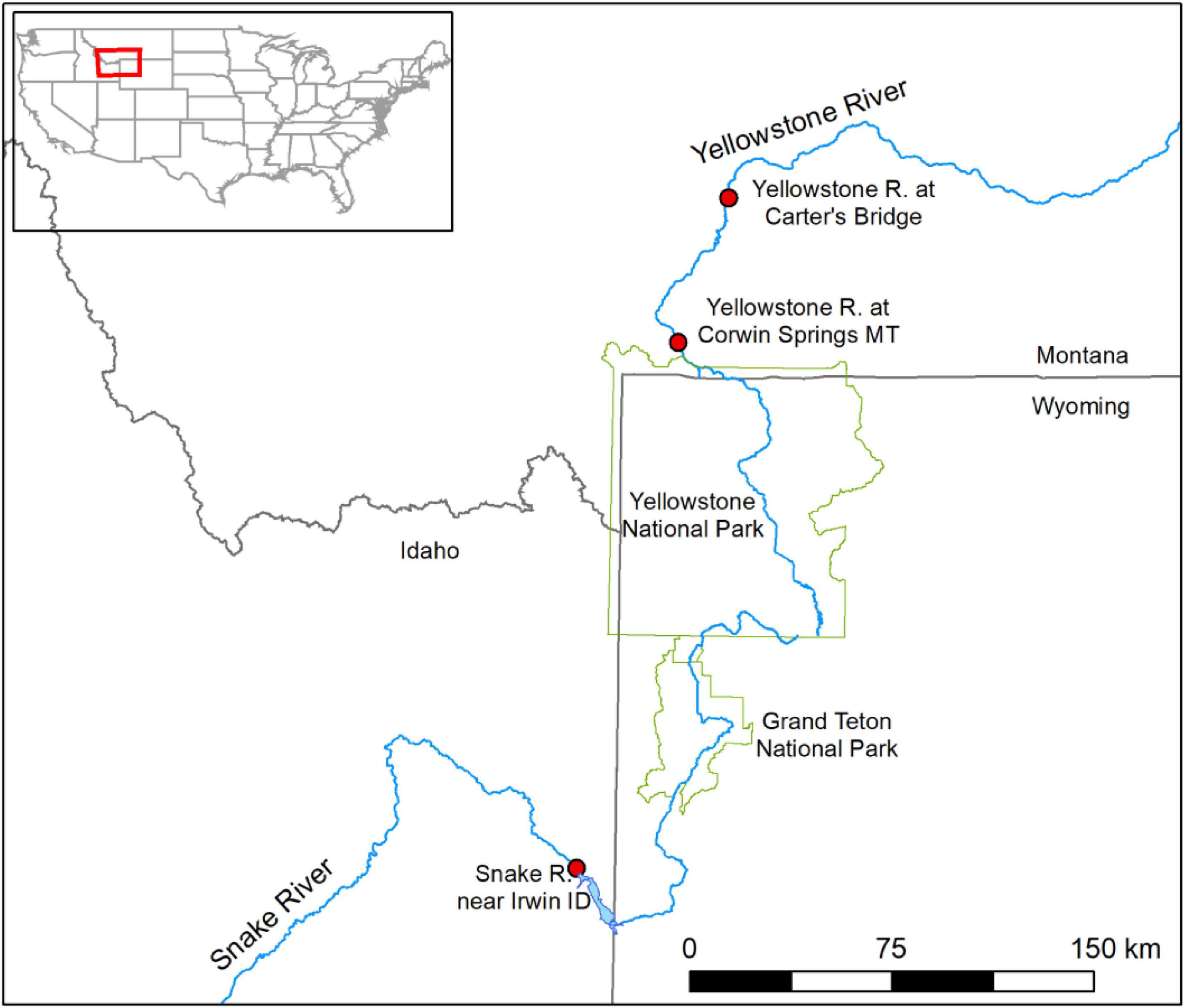
Figure 2. Map of ESP water sampling locations. The red box in the inset map shows the location of the Upper Yellowstone River and Upper Snake River in the United States. The larger map shows the sample site locations (filled red circles) on each river relative to Yellowstone National Park and Grand Teton National Park (outlined in green).
In the second dataset used as an example of eDNA monitoring programs for more common species, an autonomous robotic eDNA sampler collected water samples at one USGS streamgage on the Snake River of Idaho (United States): USGS 13032500 Snake River near Irwin ID (Figure 2). This streamgage is 1.5 km downstream of Palisades Reservoir (WY/ID). The robotic eDNA sampler was programmed to collect 2-L samples every 12 h from July 17 to September 09 and then every 4 h from September 10 to October 01, 2019. Samples were analyzed for Oncorhynchus nerka (kokanee salmon) DNA; O. nerka occur upstream in Palisades Reservoir. Thirty-five of 128 samples were scored as positive for O. nerka DNA (Sepulveda et al., 2020).
The Monterey Bay Aquarium Research Institute’s (MBARI) robotic instrument, the Environmental Sample Processor (ESP), was used to collect eDNA samples in both datasets. The ESP is a robotic device that can be programmed to automate water sample filtration and preservation of the captured material or homogenize it for immediate analyses in situ. Various iterations of the instrument have been realized over the past 25 years; eDNA samples in both datasets were collected using the “second-generation” (2G) ESP and its archival capabilities to filter water samples and preserve the collected material for later analysis in the laboratory (Scholin et al., 2017).
Details of the ESPs’ operation and eDNA analysis methods used to generate the two data sets are summarized here as they were described in Scholin et al. (2017 and references therein) and Sepulveda et al. (2020). The ESP operated autonomously, needing only power, communications and fluid connections through a waterproof pressure housing. At the initiation of sampling, a small container (a “puck”) loaded with 1.2-μm cellulose nitrate filter material was placed within a clamp. Valves opened to the outside, allowing a syringe to sequentially pull water through the puck. Once the target volume was filtered, or the filter was loaded with biomass (i.e., “clogged”), filtering stopped, and excess water was cleared. Five mL’s of RNAlater preservative was then added to the puck, soaking the filter for 10 min before excess was evacuated and the puck was returned to storage. To reduce carry-over contamination, the sampling pump, tubing and external sampling module were flushed with river water for 10 min prior to every sample collection. The sampling port of the ESP itself was cleaned with 10% bleach and a 10% Tween-20 solution between samples. Two negative controls (1 L of molecular grade water) were run through each ESP prior to and at the conclusion of each deployment to assess for contamination. Metadata associated with each sample were communicated via telemetry after each sampling point.
At the end of each ESP deployment, pucks were removed, and filters were aseptically recovered into 2.0-mL screw cap centrifuge tubes, and then shipped frozen to the USGS Upper Midwest Environmental Science Center (La Crosse, WI, United States) for DNA extraction and quantitative PCR analyses. All samples were analyzed in four replicate 25-μL reactions and tested for PCR inhibition. Samples were scored as positive when one or more PCR replicates amplified for the target DNA. Field, extraction and PCR negative controls were analyzed as regular samples; no negative controls amplified.
Abiotic Data Streams
We collated spatially and temporally explicit data from three data streams: (1) 800-m gridded climate data served from Oregon State University’s PRISM, (2) water quality data served from the National Water Quality Portal, and (3) water quantity and quality data served from the USGS water services portal. Data attributes are described in Table 1 and python scripts are available in the Supplementary Material. Spatial components of these data were delineated by the location of the eDNA sampling at USGS streamgage sites. Temporal components were reduced to daily time steps.
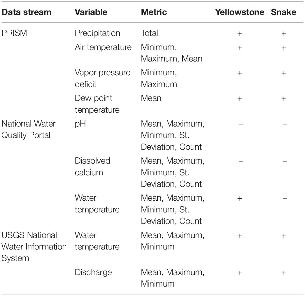
Table 1. Physical data available at daily time steps that were collated on a cloud-hosted database and then integrated with raw eDNA data in multi-scale occupancy models.
We processed and corrected the downloaded datasets. Sites with multiple observations for each day were aggregated, resulting in one average value for each site for each day. Additionally, some sites used different units of measurement such as temperature in Fahrenheit and Celsius so we standardized units across all sites and dates. In some cases, we removed white spaces from data entries to create usable numeric values. Additional columns not used in analyses were dropped from the datasets before importing data into the database.
Occupancy Analyses
We used Bayesian multi-scale occupancy models in the msocc package (Stratton et al., 2020; R version 3.5.2) to estimate the detection probability of T. bryosalmonae and O. nerka DNA, to gain insight about covariates associated with eDNA detection probability, and to estimate the effort needed for confident and high-probability detection of target eDNA. These models allow for the analysis of occupancy with three levels of hierarchical sampling, while also accounting for false negatives in detection. Models were used to estimate (1) ψ, the probability of occurrence of target eDNA at each of three streamgage sites; (2) θ the conditional probability of occurrence of target eDNA in each sample given that target eDNA was present at that site; and (3) p, the conditional probability of detection of target eDNA in each qPCR replicate of an eDNA sample given that target eDNA was present in the sample.
We used python scripts (described in the Supplementary Material) to merge our eDNA datasets with the abiotic data streams and to format and download the input data frames (detection data, site-level data with covariates, sample-level data with covariates, and replication-level data) required by the msocc package. Site-level covariates were streamgage site and date. Sample-level covariates were streamgage site, date, time, eDNA sample volume and the climate, water quality and quantity data listed in Table 1. We also added a 1-day lag to the variables listed in Table 1 to assess if eDNA detections were associated with the prior day’s conditions. We modeled p as constant since DNA extraction methods and laboratory analyses were the same for all samples.
We tested simple models that fit ψ and/or θ by each individual covariate or by combinations of covariates that were not correlated (R < 0.7, p > 0.5). We used the Watanabe-Akaike Information criterion (WAIC) to compare support for models fitted with and without covariates; models with lower WAIC values are favored (Gelman et al., 2014). We then computed estimates of the derived parameters ψ and θ for the most favored model. These estimates and their standard errors were computed using a Markov chain containing 10,000 iterations (excluding the first 1000 warm-up iterations).
Finally, we ran post-hoc power analyses to evaluate how sample size (i.e., the number of water samples and the number of PCR replicates) influenced the precision of θ estimates (msocc package, msocc_sim() as described in Stratton et al., 2020). We used the estimates of ψ, θ, and p from the most supported models of each dataset to simulate detection data. For these simulations, we varied the number of samples collected at each sampling event and the PCR replicates analyzed per sample. We then replicated this process 100 times and assessed whether the 95% credibility intervals for each parameter captured the value that generated the data. We also recorded the width of the credibility intervals. The sample sizes at which the proportion of the 95% credibility intervals that contained the original parameters stabilize and the average width of the credibility intervals stabilize provide insight about the point of diminishing returns, beyond which increasing sample size provides little benefit.
Simulations
We ran three types of simulations to assess how robotic eDNA sampling strategies can result in more detections of rare organisms and more precise estimates. In simulation 1 and 2, we explored whether high-frequency sampling can better detect target taxa DNA than lower-frequency sampling when controlling for the total number of samples. High-frequency sampling consisted of daily samples for 8 weeks; whereas lower-frequency sampling consisted of a batch of seven samples on a single day once per week for 8 weeks. We modeled two ways to think about collecting a batch of seven samples on a single day. The first approach treats the batch of samples as subsamples; in other words, the organism is present, or not, and each subsample has a probability of detecting the organism, given that it is present. The second approach treats the seven samples as independent samples, where for each sample the organism is present or not, and the sample can be detected with a given probability of the organism being present. In practice, either scenario is plausible, but it likely depends on the underlying ecological processes and how samples are collected. If the sampling process involves collecting a set of water samples at an individual location and time point, then the first approach, subsampling, may be relevant. However, if samples could be spread out over the day, and potentially space, then using independent samples may be reasonable. Data were simulated from an occupancy model framework where,
where Zi is the latent occupancy at site i, ψi is the probability that the species is present at site i, Yitj is the observed occupancy at site i, time t, and for the jth replicate, and ρit is the probability that the species will be detected at site i and time t, given presence.
Each simulated data set was summarized by whether or not a rare species was detected at least once.
In simulation 1, we used a fixed occupancy probability (ψ) and fixed detection probability (ρ) and explored the impact of different levels of ψ = {0.05, 0.10, 0.15}, ρ = {0.05, 0.10, 0.15}, and the total number of samples on a high-frequency vs. lower-frequency sampling approach. Simulation 2 was related to simulation 1 but allowed the detection probability (ρ) to vary for subsamples collected on the same day. For these subsamples, ρ varied stochastically on a day-to-day basis. Formally, Xμβ = β0 was simulated from a biased random walk such that ρ had a median value of either {0.05, 0.10, 0.15}. Code to recreate the simulations and figures is available in the Supplementary Material. The detection probability was the same for all independent samples within a day. We compared the total frequency of the sampling regimes, either daily samples for a certain number of weeks or seven samples collected for a certain number of weeks, that result in at least one detection in simulations 1 and 2.
In simulation 3, we randomly selected eDNA samples from each of the Yellowstone and Snake River datasets using the following temporal frequencies: 1 or 2 samples per day; 1, 2, or 3 samples per week; and 1 sample per month. The total number of samples differed for each time step. We replicated the random selection 100 times per time step. For each random selection, we used the msocc package to estimate θ using the null model without covariates: ψ(.), θ(.), and p(.). We compared the distributions of the 95% credibility interval widths of the θ estimates for each temporal frequency scheme.
Results
Rare Species Detection Sites
Target DNA was detected in three of 128 ESP samples at Corwin Springs and in two of 128 ESP samples at Carters Bridge. Sampling date was significantly correlated with river discharge (R = 0.90, p < 0.05). Mean air temperature was significantly correlated with minimum and maximum air temperatures (R = 0.9, p < 0.05). Models lacking time lags were more supported than those with lags.
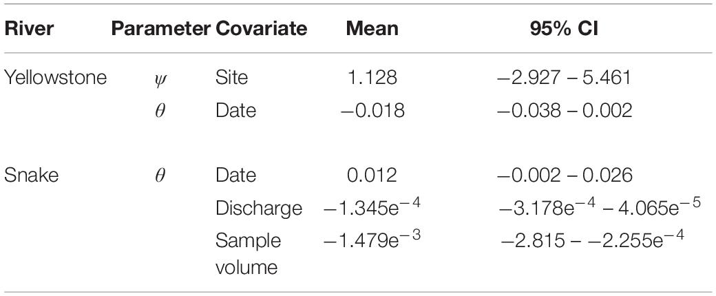
The most supported model was ψ(Site), θ(Date), p(.) (Table 2). Posterior mean estimates of ψ were higher for Corwin Springs (0.87) than for Carter’s Bridge (0.83), though confidence intervals had large overlap (Table 3). Raw estimates of the site coefficient were positive, but confidence intervals overlapped zero (Table 4). Posterior mean estimates of θ were near zero (0.02 – 0.04), but were highest on Aug 16 and lowest on Aug 08 (Table 3). There was no discernable temporal pattern in θ. Raw estimates of the date coefficient were negative, but confidence intervals overlapped zero (Table 4).
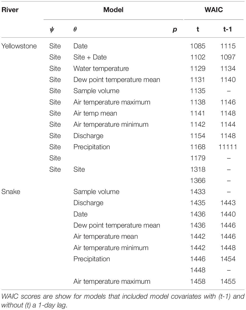
Table 2. Watanabe-Akaike information criterion (WAIC) scores of the Yellowstone and Snake river candidate models.

Table 3. Posterior mean estimates (±95% CI) of ψ, θ, and p from the candidate models with the lowest WAIC scores.
Power analyses indicated seven PCR replicates are required to reduce uncertainty in θ; the width of 95% credibility intervals for θ decreased from 0.59 at four PCR replicates to 0.05 at seven PCR replicates.
Common Species Detection Site
Target DNA was detected in 35 of 128 ESP samples. Sample date was significantly correlated with river discharge (R = −0.8, P < 0.05) and sample volume (R = −0.8, P < 0.05); river discharge and sample volume declined with sample date. River discharge and sample volume were also significantly correlated (R = 0.8, P < 0.05); smaller volumes of water were sampled when discharge was lower later in the study. Models with time lags were less supported than those without.
The most supported models included water sample volume, river discharge, or date as covariates of θ. These covariates were correlated with one another and could not be combined into a single model. Posterior mean estimates of θ increased, as water sample volume decreased, river discharge decreased, and date increased (Figure 3). Posterior mean estimates of θ ranged from 0.18 (0.08 – 0.33) to 0.58 (0.35 – 0.81) when sample volumes were 0.6 L. Raw estimates of the date coefficient were positive, while raw estimates of the discharge and sample volume coefficients were negative (Table 4). Only confidence intervals for the sample volume coefficient did not overlap zero (Table 4). Power analyses using parameters from the top three models indicated that more PCR replicates did not result in θ estimate precision gains.
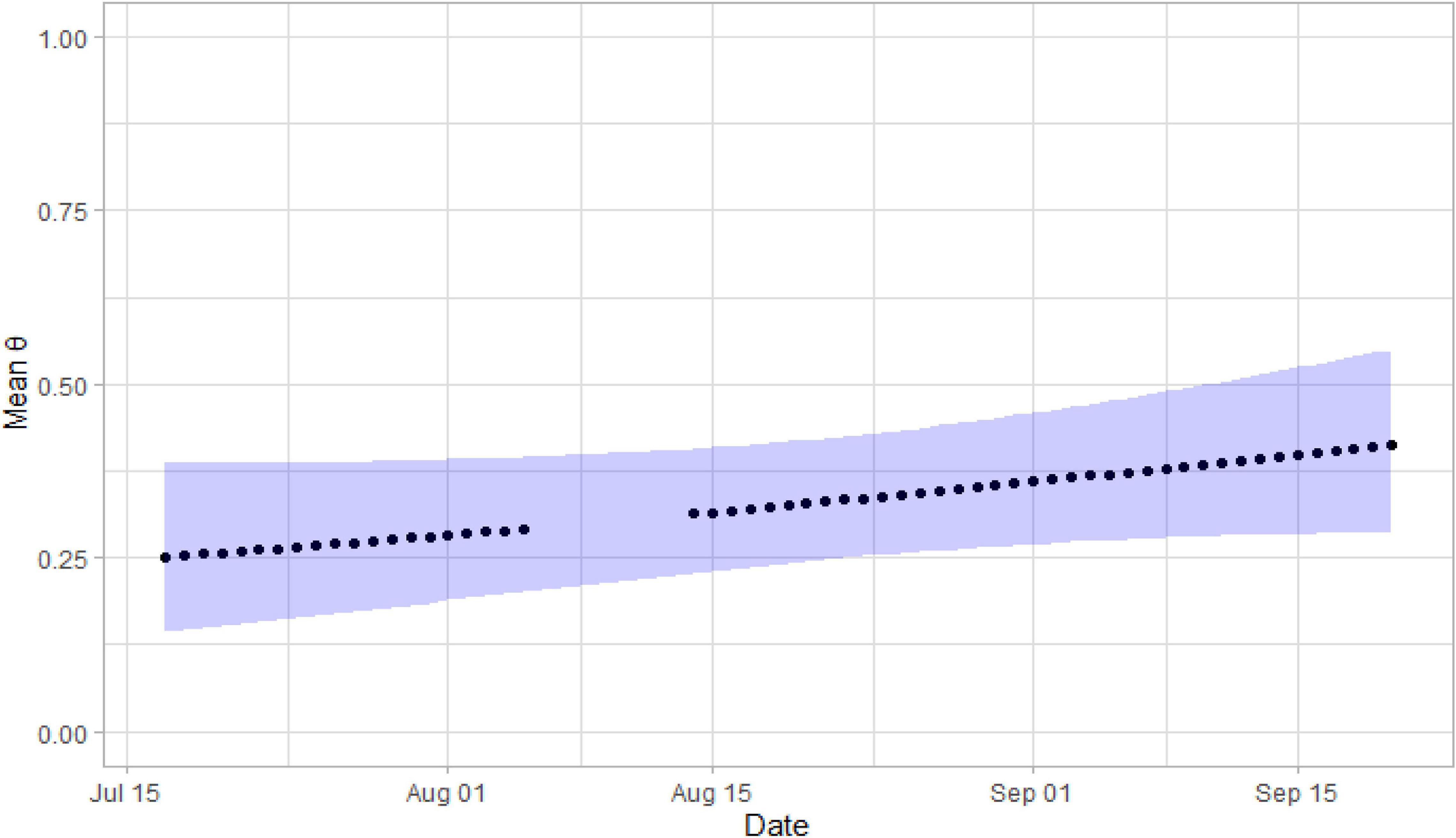
Figure 3. Posterior mean estimates of θ relative to Julian date for O. nerka DNA in the Snake River, 2019. The purple band indicates the width of the 95% confidence intervals. No sampling occurred in early August because of ESP mechanical difficulties.
Simulations
For Simulation 1, when the batch of weekly samples were considered as subsamples, high frequency sampling (i.e., daily samples) had a larger proportion of sampling schemes that resulted in at least one positive detection than lower frequency sampling (i.e., weekly samples) (Figure 4). The probability of at least one detection for daily samples was still 1−(1−ψρ)7n, but the probability of at least one detection for weekly samples is 1-[1−ψ[1−(1−ρ)7]]n. When the batch of weekly samples was considered independent, there were no discernable differences between the detection outcomes of higher vs. lower frequency sampling (Figure 5). For both daily samples and weekly batches of samples, the probability of no detection for a single sample is 1−ψρ; hence, the probability of at least one detection is 1−(1−ψρ)7n, where n is the number of weeks of sampling.
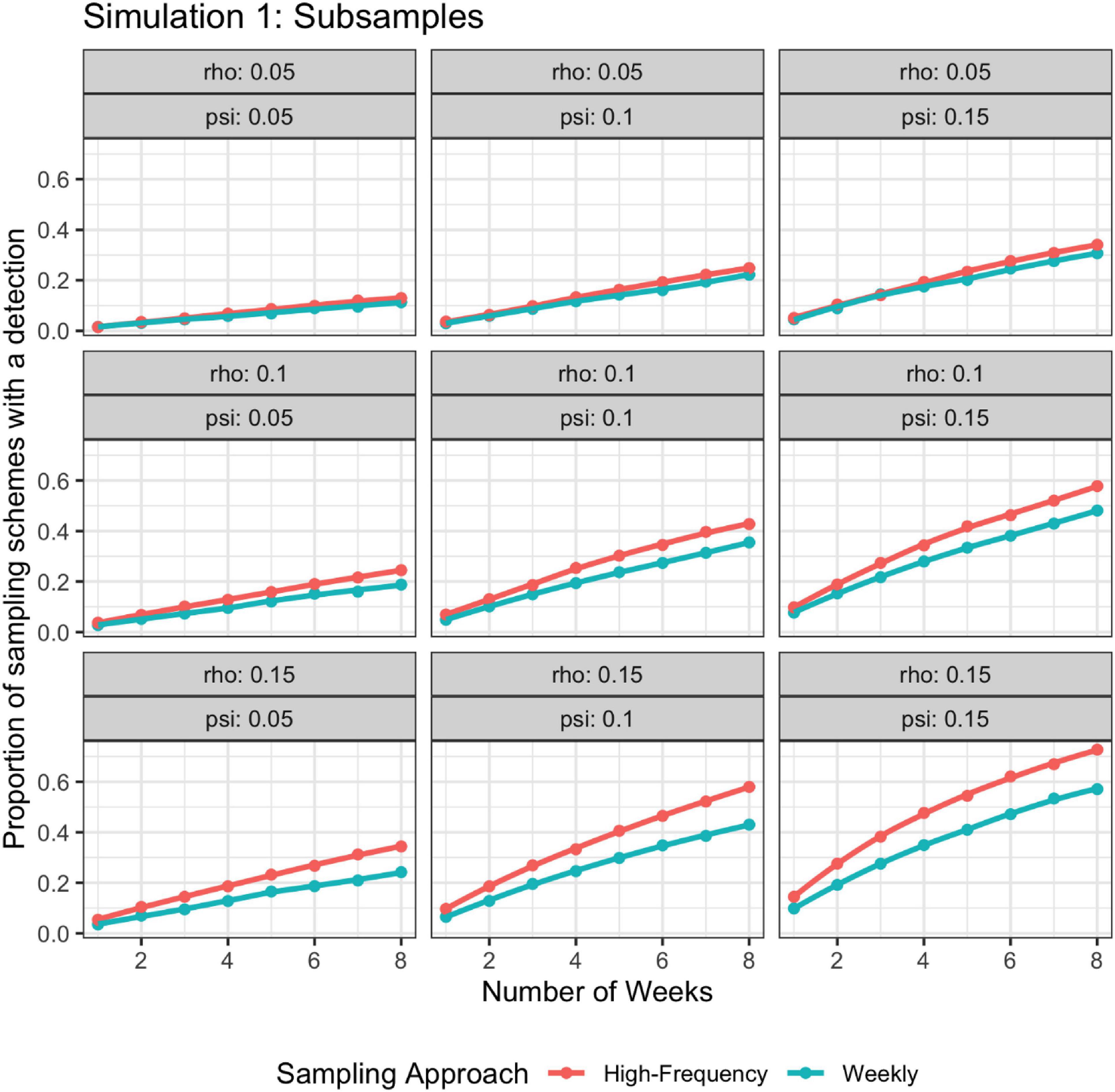
Figure 4. Probability of detection as a function of rho, psi, and number of weeks; rho does not vary by time. The high-frequency approach collects samples daily and the weekly approach takes seven samples once a week. Weekly samples are modeled as non-independent subsamples.
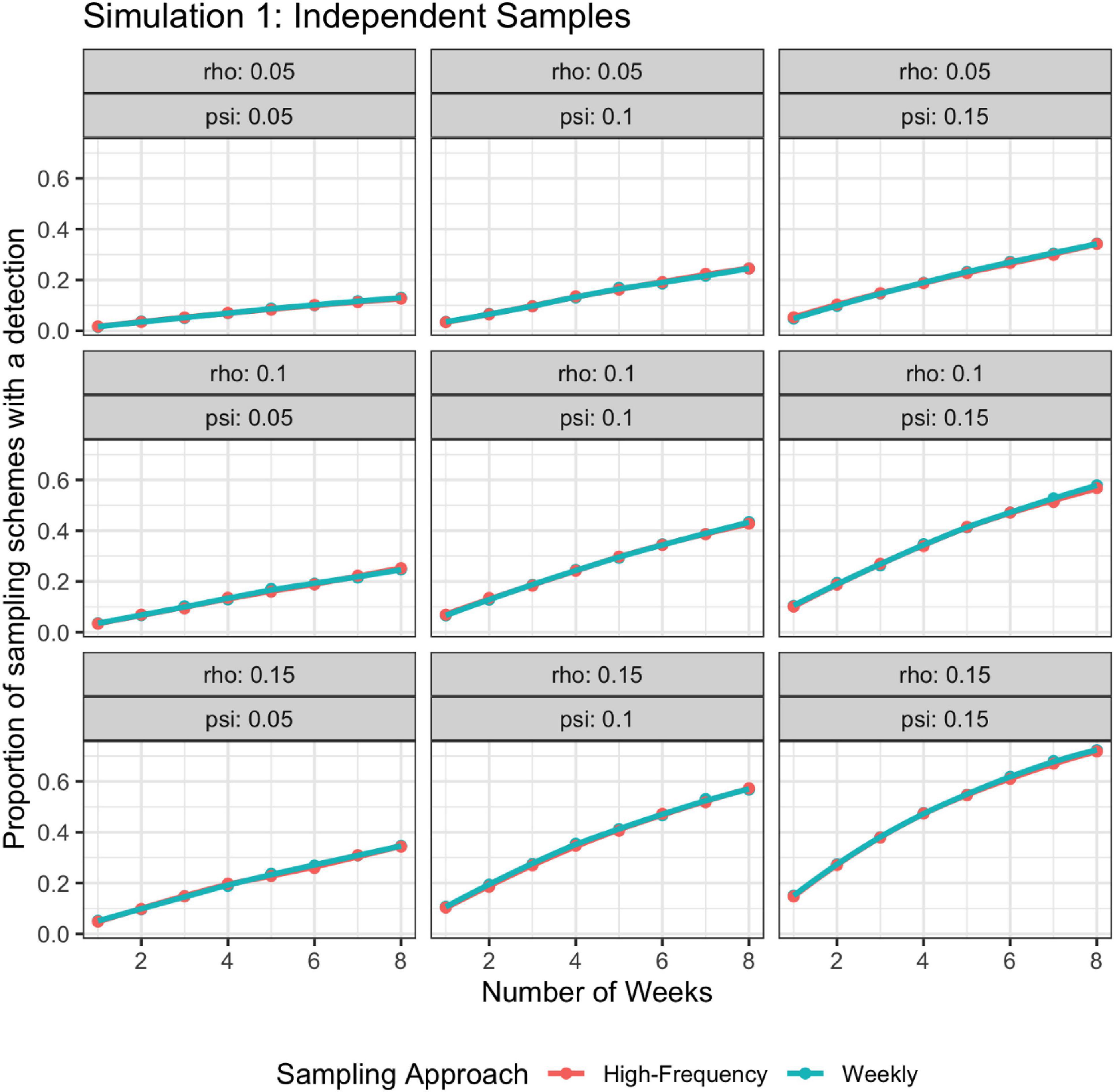
Figure 5. Probability of detection as a function of rho, psi, and number of weeks; rho does not vary by time. The high-frequency approach collects samples daily and the weekly approach takes seven samples once a week. Weekly samples are modeled as independent samples.
For simulation 2, when detection probability changed with time, the higher frequency sampling approach had a higher detection rate than the lower frequency approach regardless of if the batch of weekly samples were modeled as subsamples or independent (Figures 6, 7).
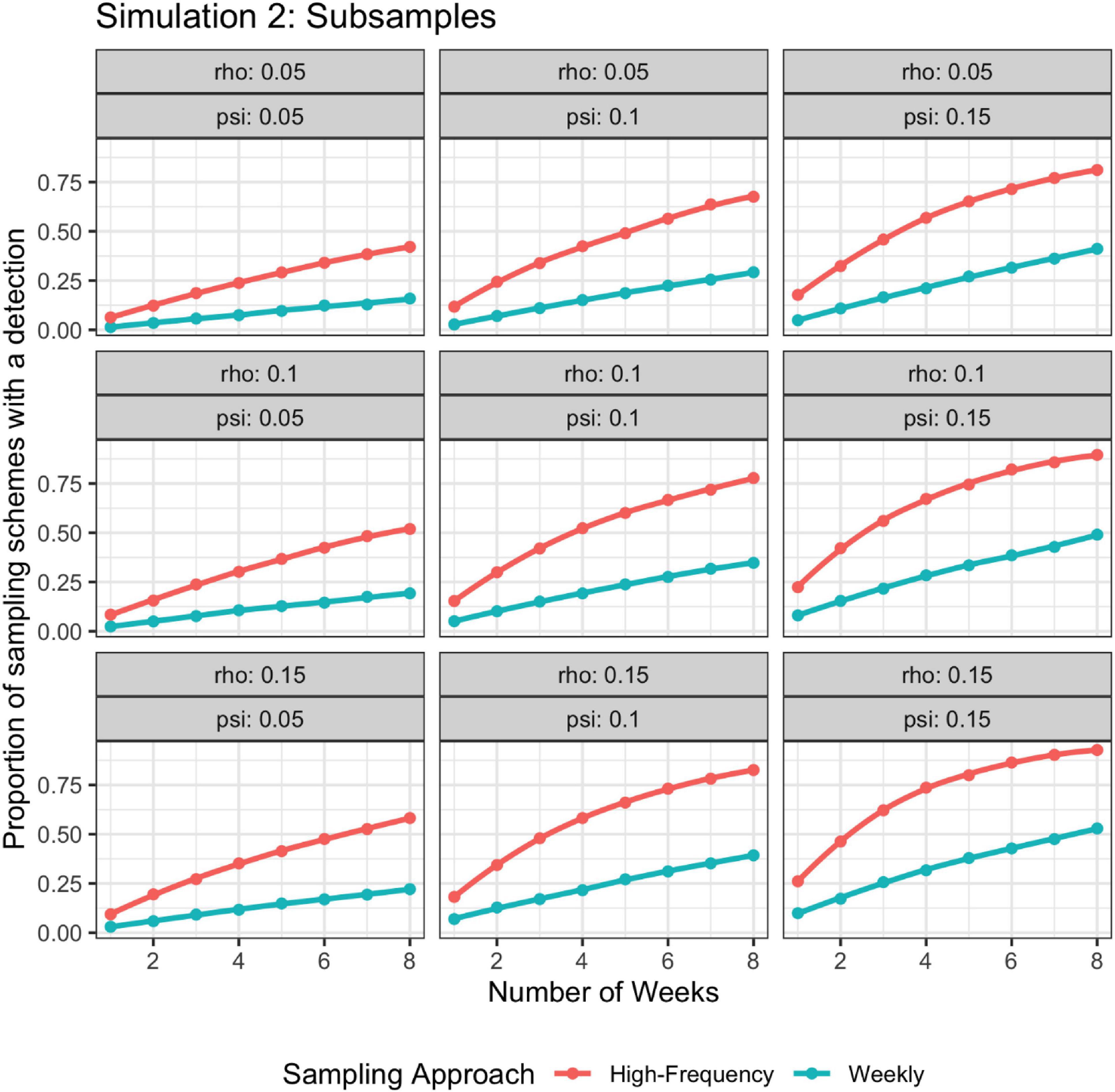
Figure 6. Probability of detection as a function of rho, psi, and number of weeks; rho varies stochastically on a day-to-day basis. The high-frequency approach collects samples daily and the weekly approach takes seven samples once a week. Weekly samples are modeled as non-independent subsamples.
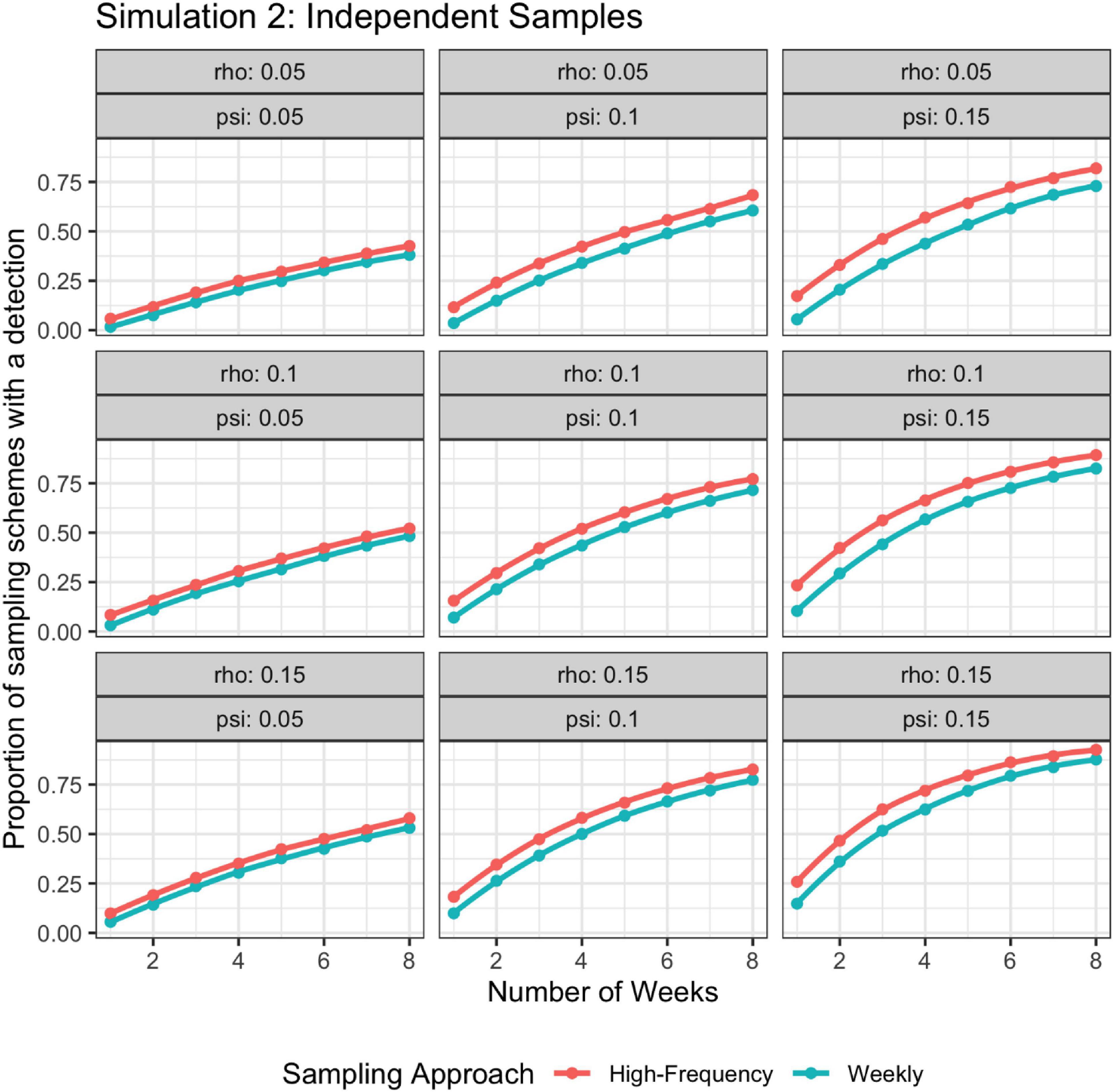
Figure 7. Probability of detection as a function of rho, psi, and number of weeks; rho varies stochastically on a day-to-day basis. The high-frequency approach collects samples daily and the weekly approach takes seven samples once a week. Weekly samples are modeled as independent samples.
For simulation 3, precision of the posterior mean θ estimates was highest (i.e., lower confidence interval width) when ESP samples were collected at least once per day in the Yellowstone River, where there were very few positive detections of the target (Figure 8). However, many of the precision values associated with these higher-frequency samples were still extremely low (i.e., higher confidence interval width), indicating that even high frequency sampling cannot reduce θ estimate uncertainty when target taxa are infrequently detected. In the Snake River, where positive detections of the target were more common, higher frequency sampling did increase precision (Figure 8). Sampling three times per week increased precision compared to sampling less frequently and sampling at least once per day increased precision compared to sampling three times per week. There were no gains in precision when sampling once vs. twice per day.
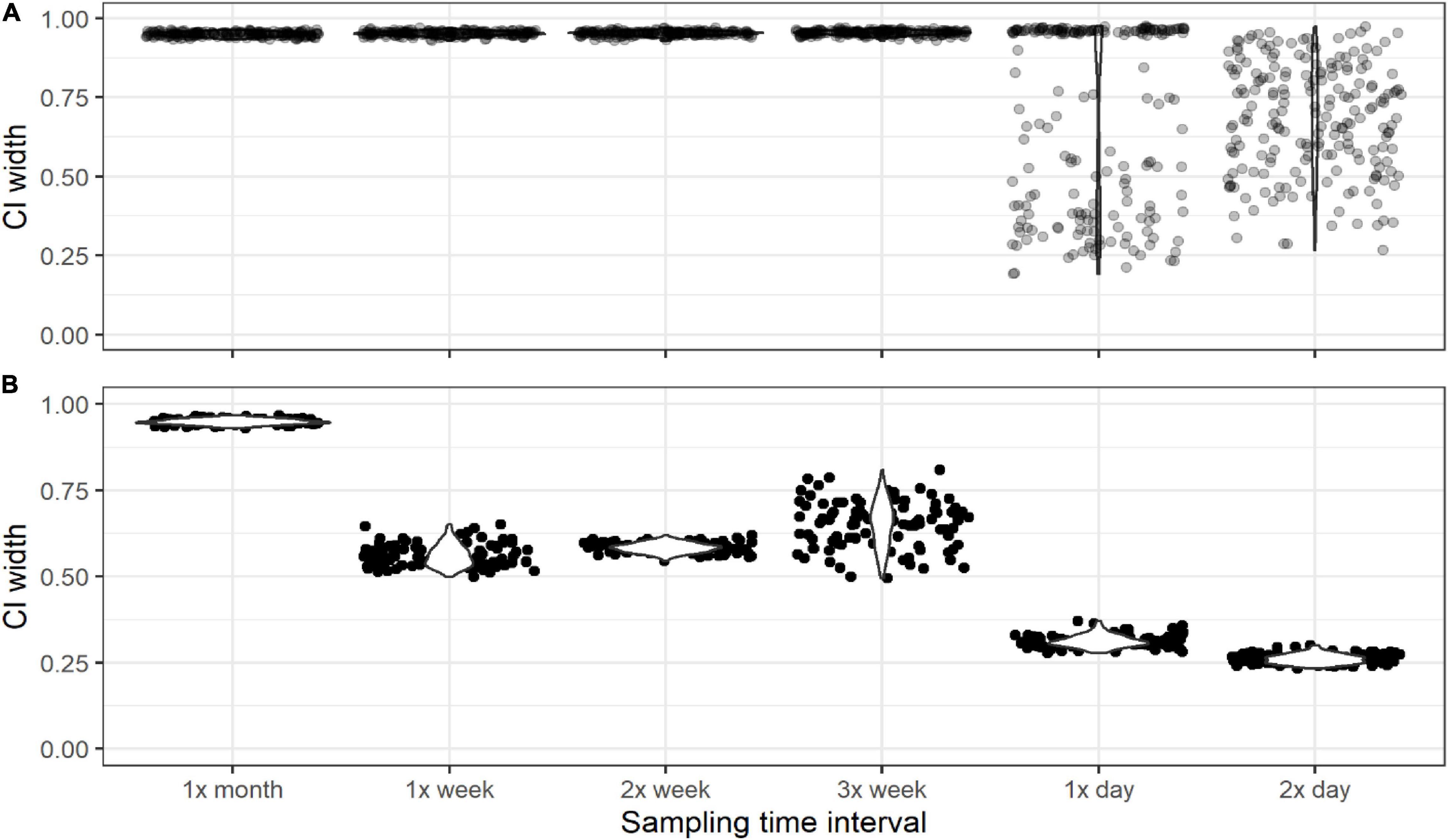
Figure 8. The difference between the 95% and 5% confidence intervals (CI width) of the posterior mean of θ for simulations of Yellowstone River (A) and Snake River (B) targets when eDNA samples were collected at different daily and weekly frequencies.
Discussion
We used data from the Yellowstone River, Montana, and the Snake River, Idaho, to demonstrate how real-time data collected by autonomous samplers and automated sensors could be integrated into a data science pipeline to provide timely information about aquatic ecosystem health. Furthermore, through simulations, we showed that data collected from autonomous samplers that enable high frequency eDNA sampling improved the accuracy and precision of inferences. Taken together, our field results and simulations indicate that rare species can be difficult to detect via eDNA sampling, and considerably more sampling may be required for detections and strong inference. Additionally, automation of the eDNA collection process and analysis of the collected data simplifies the task of data collection and repeatability of a study. Our study underscores the promise of new technologies to deliver actionable information at scales and timeframes relevant to decision makers.
Components of our analytical workflow were eDNA detection data and publicly available water-quality and climate data that were collated on a cloud-hosted database and then downloaded into data frames easily processed by computationally efficient multi-scale occupancy models (Figure 1). In our case studies, inclusion of current and lagged water quality and climate covariates did not enhance understanding of target DNA detection probabilities. Rather, T. bryosalmonae DNA detection probabilities on the Yellowstone River were associated with date of collection, and O. nerka detection probabilities on the Snake River were associated with date, discharge or water sample volume (Table 2). These results do not mean that inclusion of sensor-derived physical data is not useful for other eDNA targets, it just means that the subset of physical data analyzed were not applicable for our case studies. Inclusion of additional or alternate data sets, such as stream temperature data (U.S. Forest Service NorWeST) or other water quality, biological, and physical data collected by the USEPA [STOrage and RETrieval (STORET) Data Warehouse] for example into the analytical workflow may reveal stronger relations between parameters, particularly when used to compare detection frequencies across space rather than time.
Our multi-scale occupancy model results demonstrated that having more eDNA detections was necessary for detecting significant relations within our data. Target DNA of the fish parasite T. bryosalmonae was rarely detected in the Yellowstone River in 2018; it was likely at low abundance that year relative to previous years when PKD outbreaks were documented (Sepulveda et al., 2020; Hutchins et al.,in press). When this target was detected in a sample, it was only detected in one to two of the four PCR replicates. The large uncertainty in θ probabilities made strong associations with covariates prohibitive. Increased sampling rates (≥1 per day) did decrease confidence interval width but not to a magnitude that would be useful for confident decision making (Figure 8). This result is not a surprise nor is it unique to eDNA sampling because detection is strongly related to abundance and rare species usually have low abundance (Gaston et al., 2000). Nonetheless, this is a concerning result because eDNA sampling is championed as a superior technique for detecting rare species at low abundance, where amplification of a small subset of samples is normal (e.g., Strickland and Roberts, 2019). For example, 64 of 2822 samples tested positive for invasive Asian carp DNA (Jerde et al., 2013) and a later study found Asian carp eDNA sample detection probabilities as low as 0.04 (Mize et al., 2019). These low detection rates are the primary reason why eDNA surveys of rare species require careful consideration of field design and target species ecology (Mize et al., 2019; Strickland and Roberts, 2019). In the current study, robotic eDNA samplers were limited to the location of USGS streamgages, which were originally located for other specific purposes like recording water level. Locating robotic eDNA samplers in slow-moving waters where the T. bryosalmonae bryozoan primary host is more likely to occur, such as river pools and eddies (Wood, 2010), may have resulted in more T. bryosalmonae DNA detections. Using natural history insight of the target species to inform eDNA sampling location and timing has been recommended as a means to maximize eDNA detection probabilities of rare species (Dunker et al., 2016; Goldberg et al., 2016; Strickland and Roberts, 2019).
Comparison of multi-scale occupancy model results using the Snake River and Yellowstone River data showed that occupancy models provide the greatest benefit when sampling designs are informed by power analyses and are used in eDNA monitoring programs for established species rather than for rare species. Target DNA of O. nerka was more frequently detected in samples and replicates collected from the Snake River, especially in the fall when O. nerka was more reproductively active in the upstream reservoir (Figure 3). Collection date was correlated with river discharge and inversely correlated with sample volume. Consequently, we could not assume that date, as a surrogate for reproduction activity, was the primary driver of the eDNA detections, though this is a parsimonious explanation. Also, the Snake River streamgage is located directly below a hydropower dam at the mouth of the reservoir where O. nerka occur, so there was an increased likelihood for detection at the Snake River stream gage that was not present at the Yellowstone streamgage sites.
In addition to integrating real-time environmental data and abundant eDNA detections, our simulations illustrated that high frequency eDNA sampling has a higher probability of detection and, under certain scenarios, can provide benefits above regular, low frequency sampling. Collecting one sample every day for 7 days each week for multiple weeks (i.e., high frequency) usually resulted in more detections than collecting seven samples one day per week for multiple weeks (i.e., low frequency), especially as the target became easier to detect and ρ varied stochastically (Figures 4-7). In particular, simulation 2 allows ρ to vary stochastically in time using a random walk behavior so that detection probabilities were similar day-to-day. This mimics the situation where there might be a short window when the detection probability is considerably higher than the remainder of the sampling period. This window is not missed by sampling daily. However, under other scenarios, where the detection probability is randomly selected for a given day, there may not be substantial benefits to the high frequency sampling when treating samples as independent. Simulations in which low-frequency samples were modeled as independent rather than dependent and ρ did not vary stochastically did not show any differences between low and high-frequency sampling. High frequency sampling designs (day or night) are more easily executed by robotic samplers, given that daily travel to field sites can be cost-prohibitive. But, when a high frequency sampling design is not feasible, sampling should be spread out over a temporal extent (hours – days) when ψ and θ probabilities are not expected to change. Sample sites should also be distributed to maximize independence, as is done in the sampling of several eDNA amphibian monitoring programs, where multiple water samples are taken from different sites around a pond or wetland (e.g., Rees et al., 2014; Bedwell and Goldberg, 2020). However, in cases where large numbers of PCR replicates and samples are required for detection and reliable parameter estimation, such as in lotic environments, it may be necessary to take multiple samples from the same site at a similar time (e.g., Erickson et al., 2019; Sepulveda et al., 2019; Woldt et al., 2019).
Combining autonomously collected molecular data with environmental data collected by sensor networks into an expedient data science pipeline is the next step in the evolution of effective biosurveillance programs. Overall, our study used data collected from the Snake River and Yellowstone River as an effective proof-of-concept for using high-throughput technologies and novel data synthesis and analysis to deliver actionable information to decision makers. We have established the initial steps in creating a flexible and customizable data science pipeline for automating the movement and transformation of data and the consolidation of data from multiple sources to be used more strategically. Multiple steps of this pipeline are still in developmental stages, such as in situ eDNA analyses (Ussler et al., 2013; Hansen et al., 2020; Sepulveda et al., 2020), and other steps require further refinement. The next steps will include improved and more customizable data collection by the addition of machine learning to the robot samplers to enable adjustments while in situ, based on ongoing power analysis simulations and the incorporation of the pipeline into a decision tree with explicit criteria for determining when stakeholders should be alerted. Continuation of this work will lead to the development of a more powerful, advanced data science pipeline with the potential to link current physical drivers to future biological responses, thereby enabling forecasting of environmental health and ultimately enhancing our understanding of ecological processes and stressors.
Data Availability Statement
Publicly available datasets were analyzed in this study. This data can be found here: https://www.sciencebase.gov/catalog/item/5e41ab1ce4b0edb47be63b4a.
Author Contributions
AS, AH, JB, EB, and SC: study design and writing. AS, JB, EB, and PH: data collection. AS, AH, and CS: data analyses. All authors contributed to the article and approved the submitted version.
Funding
This work was supported by the USGS Ecosystem and Water Mission Areas, USGS National Innovation Center, and USGS Community for Data Integration.
Conflict of Interest
The authors declare that the research was conducted in the absence of any commercial or financial relationships that could be construed as a potential conflict of interest.
Acknowledgments
We thank Roman Marin III (MBARI), he was essential in getting the ESP devices to work in the USGS streamgage sites. He unexpectedly passed away prior to the completion of this project. We also thank Teton County Weed and Pest, the U.S. Bureau of Reclamation Palisades Dam, and hydro-technicians from the USGS Idaho Water Science Center for helping with robotic sampler logistics. Any use of trade, firm, or product names is for descriptive purposes only and does not imply endorsement by the U.S. Government.
Supplementary Material
The Supplementary Material for this article can be found online at: https://www.frontiersin.org/articles/10.3389/fevo.2021.620715/full#supplementary-material
References
Al-Chokhachy, R., Sepulveda, A. J., Ray, A. M., Thoma, D. P., and Tercek, M. T. (2017). Evaluating species-specific changes in hydrologic regimes: an iterative approach for salmonids in the Greater Yellowstone Area (USA). Rev. Fish Biol. Fish. 27, 425–441. doi: 10.1007/s11160-017-9472-3
Bedwell, M. E., and Goldberg, C. S. (2020). Spatial and temporal patterns of environmental DNA detection to inform sampling protocols in lentic and lotic systems. Ecol. Evol. 10, 1602–1612. doi: 10.1002/ece3.6014
Bohan, D. A., Vacher, C., Tamaddoni-Nezhad, A., Raybould, A., Dumbrell, A. J., and Woodward, G. (2017). Next-generation global biomonitoring: large-scale, automated reconstruction of ecological networks. Trends Ecol. Evol. 32, 477–487. doi: 10.1016/j.tree.2017.03.001
Collins, S. L., Bettencourt, L. M., Hagberg, A., Brown, R. F., Moore, D. I., Bonito, G., et al. (2006). New opportunities in ecological sensing using wireless sensor networks. Front. Ecol. Environ. 4:402–407. doi: 10.1890/1540-929520064[402:NOIESU]2.0.CO;2
Cordier, T., Alonso-Sáez, L., Apothéloz-Perret-Gentil, L., Aylagas, E., Bohan, D. A., Bouchez, A., et al. (2020). Ecosystems monitoring powered by environmental genomics: a review of current strategies with an implementation roadmap. Mol. Ecol. doi: 10.1111/mec.15472 [Epub ahead of print],
Cristescu, M. E., and Hebert, P. D. (2018). Uses and misuses of environmental DNA in biodiversity science and conservation. Annu. Rev. Ecol. Evol. Syst. 49, 209–230. doi: 10.1146/annurev-ecolsys-110617-062306
Darling, J. A. (2019). How to learn to stop worrying and love environmental DNA monitoring. Aquat. Ecosyst. Health Manag. 22, 440–451. doi: 10.1080/14634988.2019.1682912
Dunker, K. J., Sepulveda, A. J., Massengill, R. L., Olsen, J. B., Russ, O. L., Wenburg, J. K., et al. (2016). Potential of environmental DNA to evaluate northern pike (Esox lucius) eradication efforts: an experimental test and case study. PLoS One 11:e0162277. doi: 10.1371/journal.pone.0162277
Erickson, R. A., Merkes, C. M., and Mize, E. L. (2019). Sampling designs for landscape-level eDNA monitoring programs. Integr. Environ. Assess. Manag. 15, 760–771. doi: 10.1002/ieam.4155
Gallien, L., Münkemüller, T., Albert, C. H., Boulangeat, I., and Thuiller, W. (2010). Predicting potential distributions of invasive species: where to go from here? Divers. Distribut. 16, 331–342. doi: 10.1111/j.1472-4642.2010.00652.x
Gaston, K. J., Blackburn, T. M., Greenwood, J. J., Gregory, R. D., Quinn, R. M., and Lawton, J. H. (2000). Abundance–occupancy relationships. J. Appl. Ecol. 37, 39–59. doi: 10.1046/j.1365-2664.2000.00485.x
Gelman, A., Hwang, J., and Vehtari, A. (2014). Understanding predictive information criteria for Bayesian models. Stat. Comput. 24, 997–1016. doi: 10.1007/s11222-013-9416-2
Glibert, P. M., Pitcher, G. C., Bernard, S., and Li, M. (2018). “Advancements and continuing challenges of emerging technologies and tools for detecting harmful algal blooms, their antecedent conditions and toxins, and applications in predictive models,” in Global Ecology and Oceanography of Harmful Algal Blooms, Vol. 232, eds P. Glibert, E. Berdalet, M. Burford, G. Pitcher, and M. Zhou (Cham: Springer), 339–357. doi: 10.1007/978-3-319-70069-4_18
Goldberg, C. S., Turner, C. R., Deiner, K., Klymus, K. E., Thomsen, P. F., Murphy, M. A., et al. (2016). Critical considerations for the application of environmental DNA methods to detect aquatic species. Methods Ecol. Evol. 7, 1299–1307. doi: 10.1111/2041-210X.12595
Hansen, B. K., Jacobsen, M. W., Middelboe, A. L., Preston, C. M., Marin, R., Bekkevold, D., et al. (2020). Remote, autonomous real-time monitoring of environmental DNA from commercial fish. Sci. Rep. 10, 1–8. doi: 10.1038/s41598-020-70206-8
Hutchins, P. R., Sepulveda, A. J., Hartikainen, H. H., Staigmiller, K. D., Opitz, S., Yamamoto, R., et al. (in press). Exploration of the 2016 Yellowstone river fish kill and proliferative kidney disease in wild fish populations. Ecosphere.
Jerde, C. L., Chadderton, W. L., Mahon, A. R., Renshaw, M. A., Corush, J., Budny, M. L., et al. (2013). Detection of Asian carp DNA as part of a Great Lakes basin-wide surveillance program. Can. J. Fish. Aquat. Sci. 70, 522–526. doi: 10.1139/cjfas-2012-0478
Kovach, R. P., Dunham, J. B., Al-Chokhachy, R., Snyder, C. D., Letcher, B. H., Young, J. A., et al. (2019). An integrated framework for ecological drought across riverscapes of North America. BioScience 69, 418–431. doi: 10.1093/biosci/biz040
Michener, W. K., and Jones, M. B. (2012). Ecoinformatics: supporting ecology as a data-intensive science. Trends Ecol. Evol. 27, 85–93. doi: 10.1016/j.tree.2011.11.016
Mize, E. L., Erickson, R. A., Merkes, C. M., Berndt, N., Bockrath, K., Credico, J., et al. (2019). Refinement of eDNA as an early monitoring tool at the landscape-level: study design considerations. Ecol. Appl. 29:e01951. doi: 10.1002/eap.1951
Pilliod, D. S., Laramie, M. B., MacCoy, D., and Maclean, S. (2019). Integration of eDNA-based biological monitoring within the US Geological Survey’s National Streamgage Network. J. Am. Water Resour. Assoc. 55, 1505–1518. doi: 10.1111/1752-1688.12800
Rees, H. C., Maddison, B. C., Middleditch, D. J., Patmore, J. R., and Gough, K. C. (2014). The detection of aquatic animal species using environmental DNA–a review of eDNA as a survey tool in ecology. J. Appl. Ecol. 51, 1450–1459. doi: 10.1111/1365-2664.12306
Scholin, C. A., Birch, J., Jensen, S., Marin, R. III, Massion, E., Pargett, D., et al. (2017). The quest to develop ecogenomic sensors: a 25-year history of the Environmental Sample Processor (ESP) as a case study. Oceanography 30, 100–113. doi: 10.5670/oceanog.2017.427
Sepulveda, A. J., Birch, J. M., Barnhart, E. P., Merkes, C. M., Yamahara, K. M., Marin, R., et al. (2020). Robotic environmental DNA bio-surveillance of freshwater health. Sci. Rep. 10, 1–8. doi: 10.1038/s41598-020-71304-3
Sepulveda, A. J., Schmidt, C., Amberg, J., Hutchins, P., Stratton, C., Mebane, C., et al. (2019). Adding invasive species biosurveillance to the US Geological Survey streamgage network. Ecosphere 10:e02843. doi: 10.1002/ecs2.2843
Sepulveda, A. J., Tercek, M. T., Al-Chokhachy, R., Ray, A. M., Thoma, D. P., Hossack, B. R., et al. (2015). The shifting climate portfolio of the Greater Yellowstone Area. PLoS One 10:e0145060. doi: 10.1371/journal.pone.0145060
Stohlgren, T. J., and Schnase, J. L. (2006). Risk analysis for biological hazards: what we need to know about invasive species. Risk Anal. 26, 163–173. doi: 10.1111/j.1539-6924.2006.00707.x
Stratton, C., Sepulveda, A., and Hoegh, A. (2020). msocc: Fit and analyze computationally efficient multi-scale occupancy models in R. Methods Ecol. Evol. 11, 1113–1120. doi: 10.1111/2041-210X.13442
Strickland, G. J., and Roberts, J. H. (2019). Utility of eDNA and occupancy models for monitoring an endangered fish across diverse riverine habitats. Hydrobiologia 826, 129–144. doi: 10.1007/s10750-018-3723-8
Sugai, L. S. (2020). Pandemics and the need for automated systems for biodiversity monitoring. J. Wildl. Manag. doi: 10.1002/jwmg.21946 [Epub ahead of print],
Uden, D. R., Allen, C. R., Angeler, D. G., Corral, L., and Fricke, K. A. (2015). Adaptive invasive species distribution models: a framework for modeling incipient invasions. Biol. Invasions 17, 2831–2850. doi: 10.1007/s10530-015-0914-3
Ussler, W. III, Preston, C., Tavormina, P., Pargett, D., Jensen, S., Roman, B., et al. (2013). Autonomous application of quantitative PCR in the deep sea: in situ surveys of aerobic methanotrophs using the deep-sea environmental sample processor. Environ. Sci. Technol. 47, 9339–9346. doi: 10.1021/es4023199
Woldt, A., Baerwaldt, K., Monroe, E., Tuttle-Lau, M., Grueneis, N., Holey, M., et al. (2019). Quality Assurance Project Plan: eDNA Monitoring of Bighead and Silver Carps. Bloomington, MN: U.S. Fish and Wildlife Service.
Wood, T. S. (2010). “Bryozoans,” in Ecology and Classification of North American Freshwater Invertebrates, eds J. H. Thorp and A. P. Covich (Amsterdam: Elsevier), 437–454. doi: 10.1016/B978-0-12-374855-3.00013-3
Keywords: climate, detection, molecular, occupancy analysis, river, salmon, streamgage
Citation: Sepulveda AJ, Hoegh A, Gage JA, Caldwell Eldridge SL, Birch JM, Stratton C, Hutchins PR and Barnhart EP (2021) Integrating Environmental DNA Results With Diverse Data Sets to Improve Biosurveillance of River Health. Front. Ecol. Evol. 9:620715. doi: 10.3389/fevo.2021.620715
Received: 23 October 2020; Accepted: 18 February 2021;
Published: 16 March 2021.
Edited by:
Hiroki Yamanaka, Ryukoku University, JapanReviewed by:
William Sutton, Tennessee State University, United StatesLuca Carraro, Swiss Federal Institute of Aquatic Science and Technology, Switzerland
Copyright © 2021 Sepulveda, Hoegh, Gage, Caldwell Eldridge, Birch, Stratton, Hutchins and Barnhart. This is an open-access article distributed under the terms of the Creative Commons Attribution License (CC BY). The use, distribution or reproduction in other forums is permitted, provided the original author(s) and the copyright owner(s) are credited and that the original publication in this journal is cited, in accordance with accepted academic practice. No use, distribution or reproduction is permitted which does not comply with these terms.
*Correspondence: Adam J. Sepulveda, YXNlcHVsdmVkYUB1c2dzLmdvdg==
 Adam J. Sepulveda
 Andrew Hoegh2
 Sara L. Caldwell Eldridge
 James M. Birch
 Patrick R. Hutchins
 Elliott P. Barnhart