Can We Compare Effect Size of Spatial Genetic Structure Between Studies and Species Using Moran Eigenvector Maps?

As the field of landscape genetics is progressing toward comparative empirical studies and meta-analysis, it is important to know how best to compare the strength of spatial genetic structure between studies and species. Moran’s Eigenvector Maps are a promising method that does not make an assumption of isolation-by-distance in a homogeneous environment but can discern cryptic structure that may result from multiple processes operating in heterogeneous landscapes. MEMgene uses spatial filters from Moran’s Eigenvector Maps as predictor variables to explain variation in a genetic distance matrix, and it returns adjusted R² as a measure of the amount of genetic variation that is spatially structured. However, it is unclear whether, and under which conditions, this value can be used to compare the degree of spatial genetic structure (effect size) between studies. This study addresses the fundamental question of comparability at two levels: between independent studies (meta-analysis mode) and between species sampled at the same locations (comparative mode). We used published datasets containing 9,900 haploid, biallelic, neutral loci simulated on a quasi-continuous, square landscape under four demographic scenarios (island model, isolation-by-distance, expansion from one or two refugia). We varied the genetic resolution (number of individuals and loci) and the number of random sampling locations. We considered two measures of effect size, the MEMgene adjusted R² and multivariate Moran’s I, which is related to Moran’s Eigenvector Maps. Both metrics were highly sensitive to the number of locations, even when using standardized effect sizes, SES, and the number of individuals sampled per location, but not to the number of loci. In comparative mode, using the same Moran Eigenvector Maps for all species, even those with missing values at some sampling locations, reduced bias due to the number of locations under isolation-by-distance (stationary process) but increased it under expansion from one or two refugia (non-stationary process). More robust measures of effect size need to be developed before the strength of spatial genetic structure can be accurately compared, either in a meta-analysis of independent empirical studies or within a comparative, multispecies landscape genetic study.

Introduction

The field of landscape genetics combines methods used in population genetics, landscape ecology, and spatial statistics. In the context of widespread habitat loss and fragmentation, a main goal of this field is to assess the degree to which landscapes facilitate the movement of organism and their genes (i.e., landscape connectivity) by associating patterns of genetic differentiation with landscape features (Taylor et al., 1993; Tischendorf and Fahrig, 2000; Manel et al., 2003). This may inform conservation by identifying landscape features that constrain gene flow or corridors that promote it. However, because many landscape genetics studies aim to inform landscape management, other pre-existing factors that affect genetic drift, such as deme size, are generally not included. The applied goal of such studies thus focuses on maintaining genetic diversity and directing habitat conservation efforts to high priority areas (Manel et al., 2003; Storfer et al., 2007; Holderegger and Wagner, 2008; Balkenhol et al., 2009a,b). As such empirical studies use a variety of designs and statistical tools, inconsistencies between studies limit comparability and make unifying trends difficult to identify (Dyer, 2015).

Landscape genetic studies routinely fail to meet many assumptions of existing population genetic theory (Balkenhol and Landguth, 2011; Landguth et al., 2015), and the lack of comparability between studies makes it exceptionally difficult to develop a unifying theory specific to landscape genetics (Dyer, 2015). The landscape genetics literature was initially characterized by an abundance of review articles, followed by empirical, largely observational studies in various systems. Recently, comparative landscape genetic studies are becoming more common, where multiple species, or entire communities, are sampled at the same sampling locations (Manel and Holderegger, 2013). However, because different species may have different demographic histories and evolutionary dynamics, this could potentially confound our inferences about spatial genetic patterns of species sampled from the same landscapes. Therefore, empirical studies should only compare species with similar demographic histories and evolutionary dynamics. Simulation studies provide an avenue to test predictions about spatial genetic structure of species with known demography and evolutionary dynamics. The ability to compare accurately between studies would create the opportunity to synthesize across species, studies, and systems as a first step toward identifying unifying trends in landscape genetics.

An important next step to advance the field would be to compare the strength of spatial genetic structure, either across studies in a meta-analysis (Dyer, 2015) or between species in a comparative multispecies study. Regardless of the complexities of spatial genetic structure, studies in landscape genetics are highly varied in their sample size and study design. For example, between independent studies and within multispecies studies, there is commonly variation in sample size and spatial sampling design, genetic resolution, and the underlying population demographic history (Richardson et al., 2016). While two populations may rarely exhibit the exact same spatial genetic structure, there may be generalities regarding effect size in terms of the total amount of spatial genetic structure (Epperson et al., 2010). Standardized effect sizes (SES; Gotelli and McCabe, 2002), which use randomizations of the data to rescale the observed effect size, are increasingly used in the multivariate analysis of ecological data (Botta-Dukát, 2018) and could potentially improve our ability to compare the strength of spatial genetic structure between studies and species.

The use of spatial statistics has become more common in landscape genetics (Manel et al., 2010; Richardson et al., 2016). Many spatial statistics assume that the spatial pattern results from a single spatial process with constant mean, variance, and spatial covariance structure (second-order stationarity). Moran’s Eigenvector Maps (MEM; Dray et al., 2006) may be especially useful for comparison between studies and species as it can model spatial structure of any type (Wagner et al., 2017), including structure resulting from multiple processes in heterogeneous landscapes (Manel et al., 2010; Manel and Holderegger, 2013; Richardson et al., 2016; Klinga et al., 2019). MEMgene (Galpern et al., 2014) is a multivariate spatial analysis method that uses MEM as spatial filters to quantify the spatial structure in a matrix of genetic distances between sampling locations. It can identify and visualize spatial patterns and neighborhoods in molecular genetic data and detect cryptic spatial genetic structure that may result from isolation by distance (IBD), resistance (IBR) or environment (IBE), or a combination thereof. Within this framework, MEMgene calculates an adjusted R² that quantifies the total amount of spatial genetic structure without making assumptions about its specific form. MEM can also be used to calculate Moran’s I, a spatial statistic that is often used to quantify and test for spatial autocorrelation (Dray, 2011), though this is not currently implemented in MEMgene. Both metrics can be calculated from the same MEM analysis, but they differ in their calculation and interpretation. MEMgene’s adjusted R² shows the percent of variation in a genetic distance matrix that is explained by spatial autocorrelation, based on the set of statistically significant MEM eigenvectors used as spatial filters (Galpern et al., 2014), but it gives no further indication of spatial scale. Moran’s I does not involve significance testing but a weighting of all MEM eigenvectors according to their spatial scale, so that the metric is highest for large-scale spatial variation (Wong, 2004; Dray, 2011; Wagner and Fortin, 2015). As these measures of effect size are becoming more commonly used, the question is whether, and under which conditions, they allow comparison between landscape genetic studies. It is unclear whether their conceptual differences affect the performance of either metric as a measure of effect size, and whether their performance can be improved by using standardized effect sizes. Our study addresses the question of how to compare effect size at two levels, between independent studies and within multispecies studies, focusing on three main factors: underlaying population demography, genetic resolution, and spatial sampling design.

There is little information available on how MEMgene’s adjusted R² and Moran’s I behave across cases with variation in underlaying demographic history, which is essential to compare effect size between cases. The underlaying population demographic history is frequently more complex than a simple, stationary process such as IBD and may be the result of multiple ecological and evolutionary processes (Wagner and Fortin, 2013). For example, it is possible that the current population is the result of expansion from one or more refugia after glaciation (Lait et al., 2012; Shaw et al., 2015). Spatial genetic structure could also be affected by evolutionary processes such as drift and selection (Born et al., 2008; Gaggiotti et al., 2009). And on a more contemporary time scale, it could be affected by ecological processes that affect dispersal, and by extension, gene flow. For example, habitat loss and fragmentation may increase landscape resistance to organismal movement and thus reduce dispersal and gene flow (Cushman, 2006). These processes are commonly spatial, non-stationary, and potentially interactive. While MEM does not make an explicit assumption of stationarity, it is known to be sensitive to trend (Borcard et al., 2004; Dormann et al., 2007). IBD is stationary, but this assumption may be violated where there is IBR or expansion from glacial refugia. The empirical researcher typically has little prior knowledge of the population demographic history of their study species in their system. Therefore, in comparative landscape genetic studies, demographic history should be considered as a potential confounding variable.

Genetic resolution for the purposes of this study relates to two factors, the number of biallelic loci and the number of individuals per deme. Genetic resolution can vary in either or both factors. It is unknown if the strength of spatial genetic structure can be compared where there is variation in genetic resolution between studies. Due to their increasing popularity, our study focuses on single nucleotide polymorphisms (SNP). Non-biallelic loci, such as microsatellites, show polymorphism at each locus (Morin et al., 2004; Wong, 2004), so that highly polymorphic loci provide greater resolution (Landguth et al., 2012; Oyler-McCance et al., 2013).

Sampling design is also highly variable in landscape genetics studies (Oyler-McCance et al., 2013). Sampling can vary in the number of sampling locations and in their spatial configuration (Balkenhol and Fortin, 2015). Here, we focus on a simple random sample of locations, where each location represents a deme. Note that Moran Eigenvector Maps (MEM) are derived from eigen analysis of a weighted neighbor matrix of sampling locations (Dray et al., 2006), hence results based on MEM may be expected to be sensitive to the spatial sampling design. It is important to note that the number of sampling locations and their spatial configuration are confounded: if even a single location is dropped, the neighbor matrix will change and with it the MEM spatial filters used in MEMgene to model spatial genetic structure. This may make MEM-based measures of effect size sensitive to missing values. Ideally, in a comparative multispecies study, there would be no variation in sampling design if all species are sampled at the same locations. However, there will likely be missing values at some sampling locations for some species. Two strategies could be used in such a case: (i) MEMgene could be performed separately for each species based on a neighbor matrix of those sites where the species occurred, treating each species independently (meta-analysis mode); or (ii), the same MEM spatial filters could be used for all species, dropping observations for each species at locations where it was not found (comparative mode). As far as we know, the latter has not been applied or tested, and it is used here experimentally.

Using MEMgene (Galpern et al., 2014) to analyze simulated landscape genetics data by Lotterhos and Whitlock (2014, 2015), we studied the performance and comparability of adjusted R² and Moran’s I in various scenarios. The goal of our analyses was to assess which response metric, adjusted R² or Moran’s I, is more robust and comparable between scenarios. Specifically, we aimed to assess the behavior of adjusted R² or Moran’s I in response to variation in three factors: demographic history, genetic resolution, and sampling design. We considered four different scenarios of demographic history: the island model (IM), isolation-by-distance (IBD), and expansion from one (1R) or two refugia (2R). Genetic resolution varied in each of the two aspects; 6 or 20 individuals sampled per deme, and 500, 3,300, or 9,900 loci. Sampling design was set to either 90 random sampling locations, 60 or 30, and for those samples with 60 locations, missing locations were either retained as missing values (comparative mode) or were dropped and spatial filters were recalculated (meta-analysis mode). Before either of these measures can be used for comparative studies or meta-analyses, it is important to understand under what conditions results can be compared between species and study areas. Our study should contribute to the progress of future meta-analysis and synthesis across species, studies, and systems.

Materials and Methods

Simulated Data

We analyzed simulated data published by Lotterhos and Whitlock (2015). These data consist of 10,000 haploid, biallelic loci (representing SNPs: 9,990 neutral, 100 adaptive) on three replicate, quasi-continuous, square landscapes with 360 × 360 grid cells, each housing a deme. The simulated species has a large geographic range, high effective population size, and rapid linkage decay, with independently generated loci (Lotterhos and Whitlock, 2014). See the Supporting Information, Appendix S1 of Lotterhos and Whitlock (2014) for details of the simulator.

Variation in population demographic history was simulated under four models (Figure 1): island model (IM), isolation-by-distance (IBD), expansion from one refugium (1R) or two refugia (2R). The IM model served as a reference: its genetic structure is non-spatial, as migrants are drawn from a migrant pool independent of the distance between demes. The IBD model at equilibrium represents a stationary spatial process, whereas the 1R and 2R models are spatial and non-stationary, as allele frequencies are likely to show trend along clines. The carrying capacity per deme equaled 16, 71, and 124 for IBD, 1R and 2R, respectively. For all models except the IM, dispersal was modeled with a discretized Gaussian dispersal kernel with σ = 1.3 multiplied by cell width. The simulation controlled for global Fst by sampling at the time period when the global Fst was approximately equal to 0.05, which was reached after 1,000 generations for the 1R and 2R, 5,000 for the IM and 10,000 for the IBD model. This means that datasets are not directly comparable between demographic histories (Lotterhos and Whitlock, 2014, 2015).

FIGURE 1

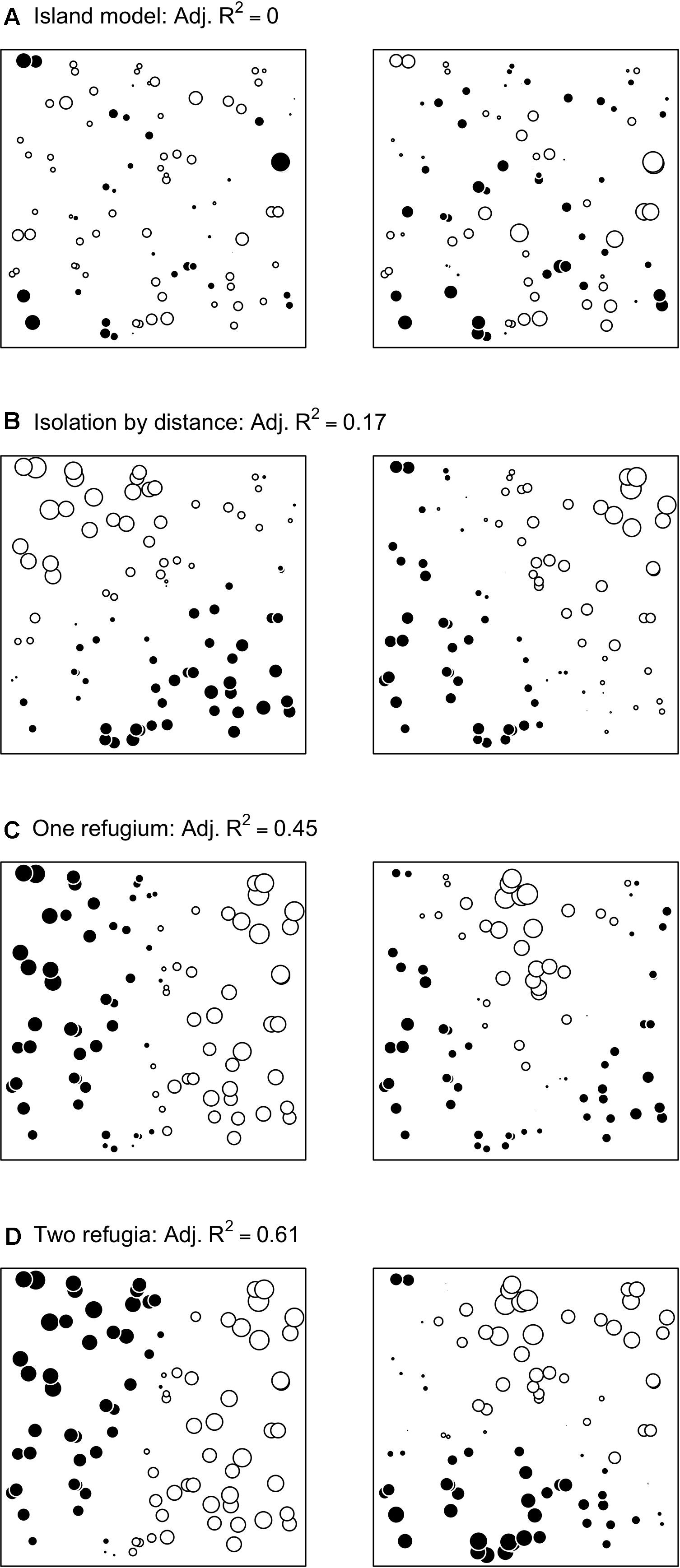
Figure 1. Visual representations (s-value plots; Galpern et al., 2014) of the first two MEMgene axes for each of the four demographic scenarios for one replicate landscape (A: island model, B: isolation by distance, C: expansion from one refugium, and D: expansion from two refugia) with the corresponding adjusted R².

Lotterhos and Whitlock (2015) sampled two sets of 6 and 20 individuals per deme, using three different sampling designs (random, transect, and pairs) with n = 90 sampling locations each. Here we used only the random samples of 90 sites. Note that the sampling locations were constant across demographic scenarios and replicate landscapes, and the spatial coordinates are available in Wagner et al. (2017).

Subsampling

For each combination of four demographic scenarios and three replicate landscapes (12 datasets), we determined deme-level allele frequencies among the 20 sampled individuals for each of the sampled 90 demes, using 9,900 neutral loci (full data). To assess the effects of genetic resolution, we repeated analyses with allele frequencies based on the sampling of 6 individuals per deme, and with a random sample of 3,300 or 500 loci. To assess the effects of the spatial sampling design, we repeated analyses for 10 random subsamples containing 60 or 30 of the original 90 sampling locations, using the same subsamples across datasets.

Genetic Analysis

For each dataset, we used the R (R Core Team, 2020) package “hierfstat” (Goudet and Jombart, 2015) to estimate sample Fst with the function “basic.stats” and calculated two pairwise genetic distance matrices (Fst: pair-wise Fst, Dch: Cavalli-Sforza and Edwards Chord distance) with the function “genet.dist” of the R package “hierfstat.”

MEMgene Analysis

MEM spatial eigenvectors were derived from Euclidean distances between sampling locations with the function “mgMEM” of the R package “memgene” (Galpern et al., 2014). We used default settings, which implement the minimum spanning tree (MST) truncation, where distances exceeding the largest distance in the MST (dMST) are replaced by 4 × dMST.

We used the function “mgForward” of the package “memgene” to select those MEM spatial eigenvectors with positive eigenvalues (i.e., representing positive spatial autocorrelation) that were significantly associated with the genetic distance matrix. We applied default settings with 100 permutations and alpha = 0.05, which is sufficient for a one-sided test.

Measures of Effect Size

We considered two main response variables, the MEMgene adjusted R² and Moran’s I. While Fst quantifies the overall genetic structure, spatial or not, the MEMgene adjusted R² quantifies how much of the overall genetic variation is spatial (Peres-Neto and Legendre, 2010; Galpern et al., 2014), and Moran’s I quantifies the degree of positive spatial autocorrelation.

The MEMgene adjusted R², as returned by the function “mgForward,” is the correlation coefficient of a distance-based redundancy analysis (dbRDA) of the genetic distance matrix regressed against the set of significant MEM spatial eigenvectors with positive spatial autocorrelation (see above), adjusted for the number of predictors (Galpern et al., 2014).

A set of n = 90 spatial locations will result in 89 MEM orthogonal spatial eigenvectors (Dray et al., 2006). Any set of n− 1 variables will be able to explain 100% of the variation in any response variable observed at the n locations. Because the MEM spatial eigenvectors are orthogonal, the correlation of each one of them with the genetic data, and thus the R² explained by each MEM spatial eigenvector, does not depend on the other eigenvectors included in the model. The total genetic variation can thus be partitioned by the MEM spatial eigenvectors, resulting in a scalogram S, a vector with n− 1 eigenvector-specific R² values that sum to 1 (Dray et al., 2012). Each MEM spatial eigenvector k represents a synthetic spatial pattern, and the MEM eigenvalue associated with eigenvector k, rescaled through dividing by a constant, is equal to Moran’s I of this pattern (Dray, 2011). Note that MEM spatial eigenvectors are sorted by their eigenvalue, from largest to smallest, thus representing a gradient from large-scale patterns, with positive spatial autocorrelation, to finest-scale patterns, with negative spatial autocorrelation. We calculated Moran’s I of the genetic data as a weighted mean of all n-1 rescaled MEM eigenvalues, weighted by the scalogram S (Dray, 2011).

In the absence of spatial autocorrelation, Moran’s I has an expected value of E(I) = −1/(n – 1). Moran’s I values vary roughly between + 1 and −1, however, the exact bounds will depend on the sampling design. Specifically, the maximum value is given by the Moran’s I of the first MEM spatial eigenvector (k = 1), and the minimum by the Moran’s I of the last MEM spatial eigenvector (k = n – 1) (Dray, 2011). Thus, Moran’s I is largest if 100% of the genetic variation is explained by the first MEM spatial eigenvector. Because we used the same n = 90 sampling locations for all datasets, the maximum value of Moran’s I was constant across the full datasets. However, each replicate subsample with 60 or 30 locations will have its own maximum value. To account for this effect, we also calculated a rescaled Moran’s I (Ir) as Ir = I/max(I).

Standardized Effect Size

Standardized effect sizes (SES) are calculated by subtracting the mean effect size (ES_sim)of R simulated data sets from the observed effect size (ES_obs) and dividing by the standard deviation (σ_sim) of the simulated values (Gotelli and McCabe, 2002):

$$\text{SES}=({\text{ES}}_{\text{obs}}-{\text{ES}}_{\text{sim}})/{\mathrm{\sigma }}_{\text{sim}}(1)$$

We simulated R = 200 datasets for each full dataset with 90 sampling locations, 20 individuals sampled per location, and 500 loci, and for each subset (with 30 or 60 sampling locations) thereof. A higher number of replicate simulations (e.g., 1,000) is generally recommended but was not feasible here due to computational constraints. The relatively low number of simulations will increase variability but is not expected to create bias in results. For each simulated dataset, genotypes of the sampled individuals were randomly permuted among the sampled locations. Then, we proceeded with the analysis as for the observed data (here, the data simulated by Lotterhos and Whitlock, 2015) to obtain an estimate of each response variable for each simulation run. The means and standard deviations among the 200 replicates were then used according to Eq. (1) to calculate SES.

We visually checked for deviations from normality of the distribution of ES_sim for the full data with 90 sampling locations under the IBD scenario. Normal probability plots for Moran’s I and rescaled Moran’s I showed no systematic deviations from normality, whereas the MEMgene adjusted R² showed a distinctly non-normal distribution with most values being zero and a few deviations in either direction. Note that the distribution did not improve when using unadjusted R² values. As deviation from normality may invalidate the use of SES (Botta-Dukát, 2018), we decided to report SES only for Moran’s I and rescaled Moran’s I.

Study Mode

To approximate a meta-analysis situation with independent analysis of multiple datasets, we performed MEMgene separately for each subsample with 60 or 30 sampling locations (meta-analysis mode). For n = 60 locations, any pair of subsamples will share at least 30 demes (50% of sampling locations), but their spatial configuration and thus MEM spatial eigenvectors will vary. While real meta-analyses will involve more independent datasets, this setting ensures that the subsamples are as comparable as possible and can be expected to exhibit similar spatial genetic structure as the full dataset with n = 90 sites, at least on average.

In a multi-species study where all species are sampled at the same locations, some species may be absent from some locations. As an alternative to performing MEMgene independently for each species (meta-analysis mode), we considered using the same, full set of 89 MEM spatial eigenvectors and dropping, for each species, the sites with missing values (comparative mode). This means that for each subsample, forward selection of MEM spatial filters with dbRDA was performed with the same predictor variables but including only the 60 observations with genetic data available. Note that because we used forward selection and included only those spatial eigenvectors with positive eigenvalues, this did not lead to overfitted models with more predictors than sites, and the adjusted R² could be calculated as above. For Moran’s I, we determined the scalogram S with a set of n – 1 simple regressions, one for each spatial eigenvector. Dropping sites is likely to render the spatial eigenvectors non-orthogonal, so that the sum of S may differ from 1. We chose not to normalize S (i.e., make it sum to 1) as preliminary results found that this led to decreased performance.

Performance Evaluation

For each dataset and response variable, we compared the value obtained for the full sample of n = 90 sampling locations to the mean value of the 10 subsamples with n = 60, which we calculated separately for the meta-analysis mode and for the comparative mode. While we expected some variability among the 10 replicate subsamples, a significant deviation of their mean from the full sample will indicate systematic bias. We used paired t-tests to statically validate such bias across datasets and evaluated effect size using Cohen’s d (Cohen, 1988).

Results

Effect of Population Demographic History

We observed considerable differences in the amount of spatial genetic structure identified for each demographic scenario by Fst, MEMgene adjusted R² (Figure 1), and Moran’s I (Figure 2). In all datasets, the demographic model where the greatest amount of genetic structure is explained by space was the 2R model, followed by 1R, and IBD. As expected, the IM showed Fst values similar to the other demographic scenarios but no spatial structure, and thus was dropped from further analysis. The difference in the strength of spatial genetic structure between the IBD, 1R, and 2R models was greater for Moran’s I than for adjusted R². This overall pattern was robust to the metric of genetic distance used, as we observed similar patterns to those based on pairwise Fst upon repeating the analysis using Dch distance (see Supplementary Figure 1).

FIGURE 2

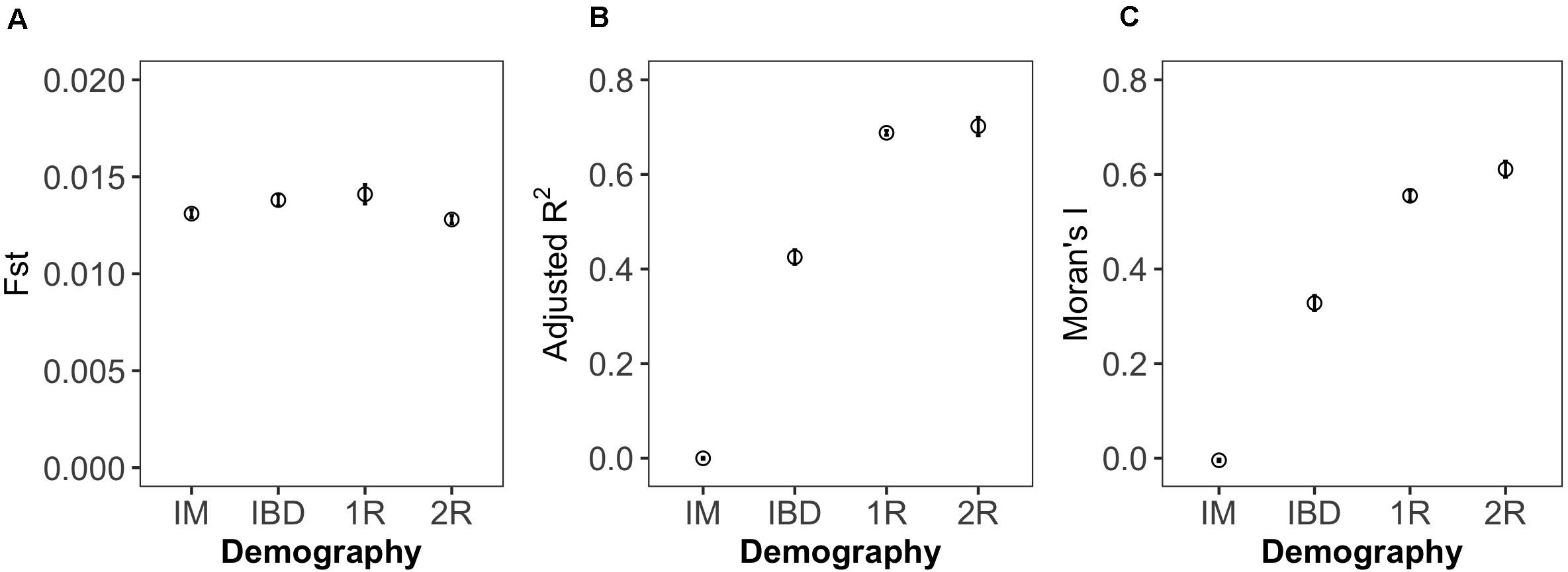
Figure 2. Effect of demographic scenario on measures of genetic structure. Each symbol shows the mean (and 95% CI) of one of three measures of genetic structure (A: Fst, B: MEM adjusted R², C: Moran’s I), averaged across three replicate datasets generated under one of four demographic scenarios (IM: island model, IBD: isolation by distance, 1R: expansion from one refugium, 2R: expansion from two refugia). Data represent all 90 sites with 20 individuals pers site genotyped at 9,900 neutral loci.

Effect of Genetic Resolution

Both adjusted R² and Moran’s I showed systematically lower values when calculated with six individuals per location, compared to 20 per location (Figure 3). In contrast, the number of loci had no discernible impact on the mean value of either response variable, though smaller numbers of loci increased variability somewhat (Figure 3). Fst was not sensitive to the number of loci or the number of individuals genotyped.

FIGURE 3

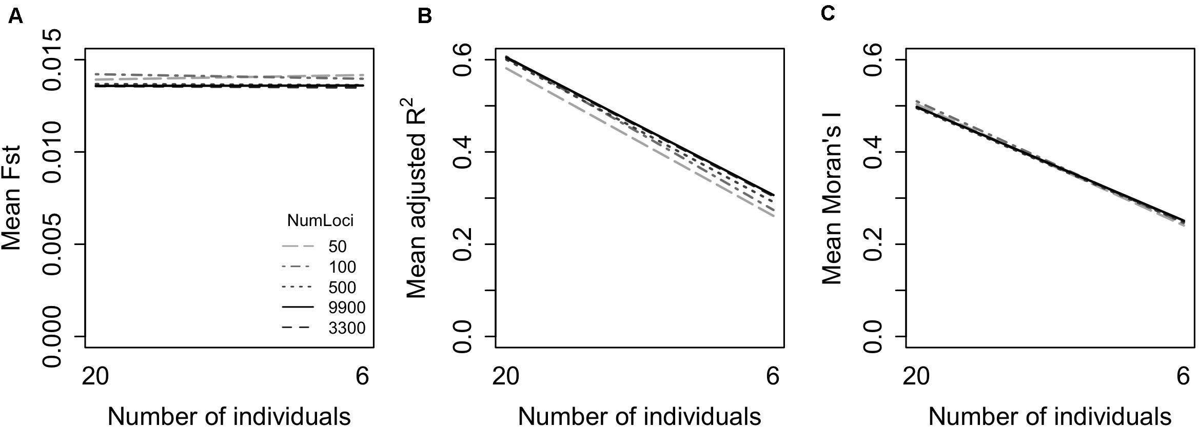
Figure 3. Effect of genetic resolution on measures of genetic structure (A: Fst, B: MEM adjusted R², C: Moran’s I). Genetic resolution was represented by variation in the number of loci (500, 3,300, or 9,900) and the number of individuals (NumInd) per site (6 or 20). Data represent all 90 sites with genetic distances based on pairwise Fst.

Effect of Spatial Sampling Design

Across all metrics, datasets with all 90 sites had higher values than those with 60, with the lowest values for those with 30 sites (Figure 4). For the IBD demographic model, meta-analysis mode (where the MEM spatial eigenvectors are derived independently for each species based on those sites where the species occurred) increased this bias compared to comparative mode (where the same MEM spatial eigenvectors are used for all species) for adjusted R² and for Moran’s I, but the opposite trend was observed for scenarios with expansion from one or two refugia. Rescaling Moran’s I by its maximum value did not eliminate bias due to the number of sampling locations (Figure 4, bottom). When comparing the mean value of the then subsamples with 30 sites to the corresponding value for the full sample of 90 sites, paired t-tests showed large, statistically significant differences, with the largest effect size (Cohen’s d) for Moran’s I, the smallest for rescaled Moran’s I, and an intermediate effect size for the MEM adjusted R² (Table 1). In meta-analysis mode, standardized effect sizes (SES), reported for Moran’s I and rescaled Moran’s I (Figure 4), were equally biased as unstandardized values when comparing effect sizes between datasets with 90, 60, or 30 sampling locations. In comparative mode, SES performed considerably worse.

FIGURE 4

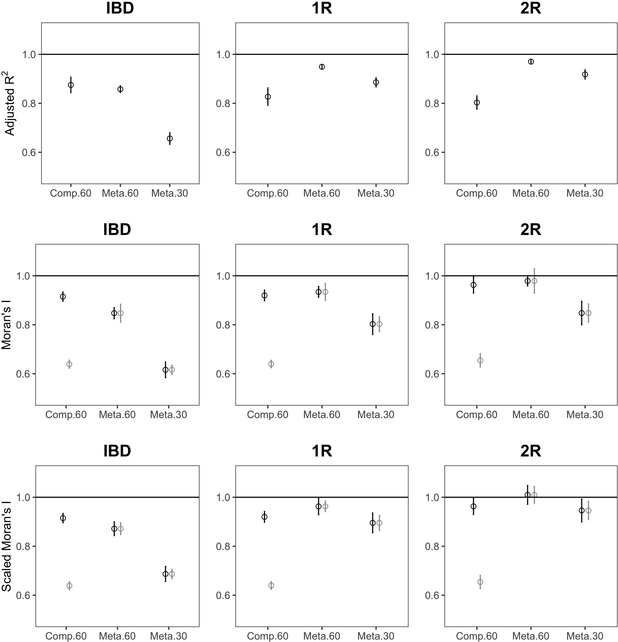
Figure 4. Effect of the spatial sampling design on measures of spatial genetic structure. Each symbol shows the relative mean (and 95% CI) of adjusted R² (top) Moran’s I (center) or scaled Moran’s I (bottom), in comparative mode with 60 sites (Comp.60), meta-analysis mode with 60 sites (Meta.60), or meta-analysis mode with 30 sites (Meta.30), for a demographic model (IBD: isolation by distance, 1R: expansion from one refugium, 2R: expansion from two refugia). Observed statistics are shown in black, those for SES in gray. Relative means were obtained by dividing the mean of 10 replicate subsamples by the value obtained for the full dataset with 90 sampling locations, so that e.g., a relative mean of 0.8 would indicate a 20% lower average than expected from the full dataset. The horizontal lines indicate a relative mean of 1. Genetic distances were based on pairwise Fst using 20 individuals per location.

TABLE 1

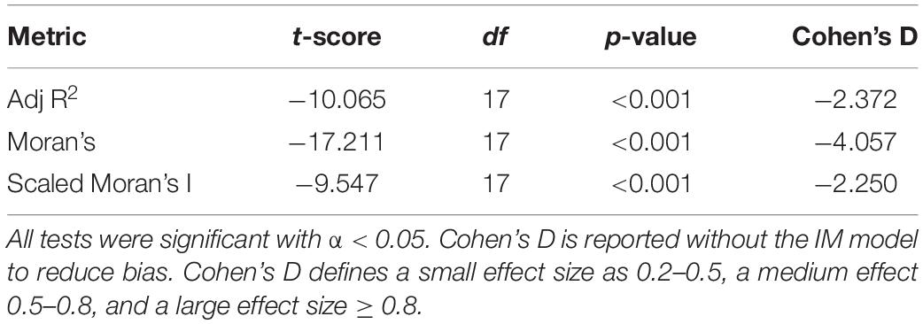
Table 1. Results of paired t-tests comparing subsamples of 30 and 90 locations for adjusted R², Moran’s I, and rescaled Moran’s I.

Discussion

Effect of Population Demographic History

We found that expansion from one or two refugia resulted in much larger effect sizes for the strength of spatial genetic structure (i.e., MEM adjusted R² and Moran’s I values), although the datasets had been simulated with comparable overall genetic differentiation (Fst). These results suggest that we cannot accurately compare the effect of landscape features on gene flow between independent studies or within a multispecies study where there is variation in underlaying population demographic history. The underlaying population demography is typically unknown to the empirical researcher and may vary between landscapes for the same species and between species for the same landscape, which further increases the uncertainty of the potential comparison between studies or species.

The strong increase of adjusted R² and Moran’s I for scenarios with expansion from one or two refugia suggests that effect size in MEMgene is sensitive to non-stationarity. It is well known that several MEM spatial filters are required to model linear trend, hence one strategy is to detrend data (Borcard et al., 2004, 2018; Griffith and Peres-Neto, 2006; Beale et al., 2010). As the response is a matrix of genetic distances, detrending is not trivial. One approach would be to detrend the allele frequencies. While relative frequencies vary between 0 and 1, removing the mean (modeled as a function of spatial x- and y-coordinates) will result in some negative values, which makes it problematic to calculate genetic distances. On the other hand, one could partial out the spatial x- and y-coordinates during spatial filtering. However, this would likely render the spatial filters non-orthogonal. When we partial out the spatial coordinates from the correlation between the genetic distances and MEM spatial eigenvectors, we regress both on the coordinates and correlate their residuals (Legendre and Legendre, 2012). The residuals of the spatial eigenvectors are no longer uncorrelated. For the sampling design in Figure 1, for instance, the pairwise correlations among the residual eigenvectors range between −0.4 < r < 0.4.

Furthermore, trend in allele frequencies, such as along a cline, may represent biologically meaningful population genetic structure, so that its elimination could also distort comparisons between studies. Further research is needed to assess whether expansion from refugia creates other forms of non-stationarity beyond trend in allele frequencies. It is also important to recognize that this study only examined two metrics based on MEM and that other methods with different assumptions may be more robust between comparisons.

Effect of Genetic Resolution

We found that both adjusted R² and Moran’s I were surprisingly robust to the number of loci, but sensitive to the number of individuals sampled per site. This is in contrast to Fst, which was robust to both changes in the number of samples per location and the number of loci. Our findings contrast with those of Landguth et al. (2012), who found that the partial Mantel r correlations between genetic and ecological distances (accounting for geographic distances) was sensitive to the number of loci and the level of polymorphism but robust to the number of individuals (with one individual sampled per location). This suggests that existing recommendations on resource allocation (i.e., when to invest into sampling more sites, genotyping more individuals per site, or increasing the number or polymorphism of genetic markers) for landscape genetic studies (Landguth et al., 2012; Oyler-McCance et al., 2013) may need to be revisited to clarify which factors are most important depending on the research question and the chosen analysis approach (Balkenhol and Fortin, 2015).

This study only examined neutral SNPs, and expanding into other common genetic markers (Hall and Beissinger, 2014), such as microsatellites, or markers under selection is beyond the scope of this study. However, in empirical datasets, other factors likely to occur (e.g., site polymorphism, strength of selection, linkage to sites under selection) may have an effect on genetic resolution. Our results suggest that the statistical power of MEMgene analysis may be more dependent on the number of individuals sampled per deme than on the number of loci. Further research should address whether sampling more individuals per location, or pooling nearby samples, increases the ability of MEMgene to detect cryptic spatial structure.

Effect of Spatial Sampling Design

We found that smaller samples (i.e., subsamples with 60 or 30 of the original 90 sampling locations) resulted in systematically lower estimates of spatial genetic structure, both for the MEMgene adjusted R² and for Moran’s I. This sensitivity to the number of sampling locations suggests difficulty in comparing between landscape genetic studies in meta-analyses. Moreover, such bias in effect size may not be limited to the analysis of genetic variation with MEMgene but could affect other applications of MEM to univariate or multivariate ecological data (Dray et al., 2012). More generally, Moran’s I has been shown to underestimate spatial autocorrelation for small numbers of spatial locations (Carrijo and da Silva, 2017).

Analysis with comparative mode, where the same basis set of MEM spatial eigenvectors (based on all sites) are used for all species, somewhat reduced bias under the stationary scenario of isolation-by-distance but increased it under the non-stationary scenarios with expansion from one or two refugia. Where there is a small number of missing sites, it may be safer to restrict analysis to those sites where all species occurred. We do not recommend using comparative mode analysis, as the bias reduction was insufficient and dependent on stationarity. In addition, there are methodological concerns where the missing observations change the correlation structure of the MEM spatial eigenvectors resulting in scalograms that do not sum to 1.

Standardized effect sizes (SES) did not provide an improvement. First, non-normal distributions among permuted datasets precluded the calculation of SES for the MEMgene adjusted R². Second, SES for subsamples in meta-analysis mode, on average, showed the same bias compared to SES for the full dataset with 90 sampling locations as observed Moran’s I (or rescaled Moran’s I). Finally, comparative mode analysis further decreased the performance of SES.

This study only examined a random sampling design with randomized missing values. While we suspect similar problems will occur with other common sampling designs, such as transects or grids (Oyler-McCance et al., 2013), those analyses are beyond the scope of this paper.

Conclusion

We found that the MEMgene adjusted R² and Moran’s I are sensitive to variation in population demographic history, the number of individuals sampled per location, and the number and spatial configuration of sampling sites. Further research will be needed to assess the sensitivity of other applications of MEM, e.g., for ecological data (Dray et al., 2006, 2012; Franckowiak et al., 2017; Bauman et al., 2018) to the number and spatial configuration of sampling locations. Additionally, it is important to keep in mind, as with any simulation study, that our simulated species is highly simplified and that species in the real world will likely vary in demography, life history, and a variety of other factors, which may further complicate analysis.

We caution those hoping to perform meta-analysis or comparative analyses with landscape genetic datasets. While MEM can model complex spatial patterns (Dray et al., 2012) and MEMgene facilitates visual comparisons of multivariate genetic data, our results suggest that the strength of spatial genetic structure cannot be easily compared using MEMgene adjusted R² or Moran’s I. Meta-analysis and multispecies studies are highly useful, particularly in studies related to habitat connectivity and climate change. However, at this point, MEM-based comparisons of the strength of spatial genetic structure between different studies or within a multispecies study will likely not be accurate. Any alternative indicator for comparison should be scrutinized for sensitivity to the underlaying population demography, genetic resolution, and sampling design before it is applied in meta-analysis and multispecies studies.

Data Availability Statement

The datasets analyzed by this study can be found in the Dryad repository (doi: 10.5061/dryad.v8d05).

Author Contributions

CH, HAM, and HW conceived the study. CH wrote the manuscript with HW contributing sections of the Methods. Statistical analyses were programmed by HW and figures were generated by HAM. HAM maintained the project code and repository on GitHub. All authors commented on the manuscript.

Funding

This research was supported by the Natural Sciences and Engineering Council of Canada (NSERC) through a Discovery Grant to HW and the CREATE program “ADVENT/ENVIRO.” The study was further supported by the Centre for Urban Environments Postdoctoral Fellowship awarded to HAM.

Conflict of Interest

The authors declare that the research was conducted in the absence of any commercial or financial relationships that could be construed as a potential conflict of interest.

Acknowledgments

We would like to acknowledge and thank K. Lotterhos and M. C. Whitlock for their simulated datasets and B. Forester for discussions about the data. We thank our funding sources NSERC, CREATE and CUE. We thank the reviewers and the handling editor for the feedback and helpful suggestions.

Supplementary Material

The Supplementary Material for this article can be found online at: https://www.frontiersin.org/articles/10.3389/fevo.2021.612718/full#supplementary-material

References

Balkenhol, N., and Fortin, M. J. (2015). “Basics of study design: sampling landscape heterogeneity and genetic variation for landscape genetic studies,” in Landscape Genetics, eds N. Balkenhol, S. A. Cushman, A. T. Storfer, and L. P. Waits (Chichester: John Wiley & Sons, Ltd), 58–76. doi: 10.1002/9781118525258.ch04

CrossRef Full Text | Google Scholar

Balkenhol, N., Gugerli, F., Cushman, S. A., Waits, L. P., Coulon, A., Arntzen, J. W., et al. (2009a). Identifying future research needs in landscape Genetics: where to from Here? Landsc. Ecol. 24, 455–463. doi: 10.1007/s10980-009-9334-z

CrossRef Full Text | Google Scholar

Balkenhol, N., and Landguth, E. L. (2011). Simulation modelling in landscape genetics: on the need to go further. Mol. Ecol. 20, 667–670. doi: 10.1111/j.1365-294X.2010.04967.x

PubMed Abstract | CrossRef Full Text | Google Scholar

Balkenhol, N., Waits, L. P., and Dezzani, R. J. (2009b). Statistical approaches in landscape genetics: an evaluation of methods for linking landscape and genetic data. Ecography 32, 818–830. doi: 10.1111/j.1600-0587.2009.05807.x

CrossRef Full Text | Google Scholar

Bauman, D., Drouet, T., Fortin, M. J., and Dray, S. (2018). Optimizing the choice of a spatial weighting matrix in eigenvector-based methods. Ecology 99, 2159–2166. doi: 10.1002/ecy.2469

PubMed Abstract | CrossRef Full Text | Google Scholar

Beale, C. M., Lennon, J. J., Yearsley, J. M., Brewer, M. J., and Elston, D. A. (2010). Regression analysis of spatial data. Ecol. Lett. 13, 246–264. doi: 10.1111/j.1461-0248.2009.01422.x

PubMed Abstract | CrossRef Full Text | Google Scholar

Botta-Dukát, Z. (2018). Cautionary note on calculating standardized effect size (SES) in randomization test. Commun. Ecol. 19, 77–83.

Google Scholar

Borcard, D., Gillet, F., and Legendre, P. (2018). Numerical Ecology with R. Cham: Springer.

Google Scholar

Borcard, D., Legendre, P., Avois-Jacquet, C., and Tuomisto, H. (2004). Dissecting the spatial structure of ecological data at multiple scales. Ecology 85, 1826–1832. doi: 10.1890/03-3111

CrossRef Full Text | Google Scholar

Born, C., Hardy, O. J., Chevallier, M. H., Ossari, S., Attéké, C., Wickings, E. J., et al. (2008). Small-scale spatial genetic structure in the central african rainforest tree species Aucoumea Klaineana: a stepwise approach to infer the impact of limited gene dispersal, population history and habitat fragmentation. Mol. Ecol. 17, 2041–2050. doi: 10.1111/j.1365-294X.2007.03685.x

PubMed Abstract | CrossRef Full Text | Google Scholar

Carrijo, T. B., and da Silva, A. R. (2017). Modified Moran’s I for small samples. Geogr. Anal. 49, 451–467. doi: 10.1111/gean.12130

CrossRef Full Text | Google Scholar

Cohen, J. (1988). Statistical Power Analysis for the Behavioral Sciences, 2nd Edn. Hillsdale, NJ: Lawrence Erlbaum Associates.

Google Scholar

Cushman, S. A. (2006). Effects of habitat loss and fragmentation on amphibians: a review and prospectus. Biol. Conserv. 128, 231–240. doi: 10.1016/j.biocon.2005.09.031

CrossRef Full Text | Google Scholar

Dormann, C. F., McPherson, J. M., Araújo, M. B., Bivand, R., Bolliger, J., Carl, G., et al. (2007). Methods to account for spatial autocorrelation in the analysis of species distributional data: a review. Ecography 30, 609–628. doi: 10.1111/j.2007.0906-7590.05171.x

CrossRef Full Text | Google Scholar

Dray, S. (2011). A new perspective about Moran’s coefficient: spatial autocorrelation as a linear regression problem. Geogr. Anal. 43, 127–141. doi: 10.1111/j.1538-4632.2011.00811.x

CrossRef Full Text | Google Scholar

Dray, S., Legendre, P., and Peres-Neto, P. R. (2006). Spatial modelling: a comprehensive framework for principal coordinate analysis of neighbour matrices (PCNM). Ecol. Modell. 196, 483–493. doi: 10.1016/j.ecolmodel.2006.02.015

CrossRef Full Text | Google Scholar

Dray, S., Pélissier, R., Couteron, P., Fortin, M. J., Legendre, P., Peres-Neto, P. R., et al. (2012). Community ecology in the age of multivariate multiscale spatial analysis. Ecol. Monogr. 82, 257–275. doi: 10.1890/11-1183.1

CrossRef Full Text | Google Scholar

Dyer, R. J. (2015). Is there such a thing as landscape genetics? Mol. Ecol. 24, 3518–3528. doi: 10.1111/mec.13249

PubMed Abstract | CrossRef Full Text | Google Scholar

Epperson, B. K., McRae, B. H., Scribner, K. T., Cushman, S. A., Rosenberg, M. S., Fortin, M. J., et al. (2010). Utility of computer simulations in landscape genetics. Mol. Ecol. 19, 3549–3564. doi: 10.1111/j.1365-294X.2010.04678.x

PubMed Abstract | CrossRef Full Text | Google Scholar

Franckowiak, R. P., Panasci, M., Jarvis, K. J., Acuña-Rodriguez, I. S., Landguth, E. L., Fortin, K. J., et al. (2017). Model selection with multiple regression on distance matrices leads to incorrect inferences. PLos One 12:e0175194. doi: 10.1371/journal.pone.0175194 Edited by Duccio Rocchini

PubMed Abstract | CrossRef Full Text | Google Scholar

Gaggiotti, O. E., Bekkevold, D., Jørgensen, H. B. H., Foll, M., Carvalho, G. R., Andre, C., et al. (2009). Disentangling the effects of evolutionary, demographic, and environmental factors influencing genetic structure of natural populations: Atlantic herring as a case study. Evolution 63, 2939–2951. doi: 10.1111/j.1558-5646.2009.00779.x

PubMed Abstract | CrossRef Full Text | Google Scholar

Galpern, P., Peres-Neto, P. R., Polfus, J., and Manseau, M. (2014). MEMGENE: spatial pattern detection in genetic distance data. Methods Ecol. Evol. 5, 1116–1120. doi: 10.1111/2041-210X.12240

CrossRef Full Text | Google Scholar

Gotelli, N. J., and McCabe, D. J. (2002). Species co-occurrence: a meta-analysis of J. M. Diamond’s assembly rules model. Ecology 83, 2091–2096.

Google Scholar

Goudet, J., and Jombart, T. (2015). hierfstat: Estimation and Tests of Hierarchical F-Statistics. R package version 0.04-22, Vol. 10.

Google Scholar

Griffith, D. A., and Peres-Neto, P. R. (2006). Spatial modeling in ecology: the flexibility of eigenfunction spatial analyses. Ecology 87, 2603–2613.

Google Scholar

Hall, A., and Beissinger, S. R. (2014). A practical toolbox for design and analysis of landscape genetics studies. Landsc. Ecol. 29, 1487–1504. doi: 10.1007/s10980-014-0082-3

CrossRef Full Text | Google Scholar

Holderegger, R., and Wagner, H. H. (2008). Landscape genetics. BioScience 58, 199–207. doi: 10.1641/b580306

CrossRef Full Text | Google Scholar

Klinga, P., Mikoláš, M., Smolko, P., Tejkal, M., Höglund, J., and Paule, L. (2019). Considering landscape connectivity and gene flow in the anthropocene using complementary landscape genetics and habitat modelling approaches. Landsc. Ecol. 34, 521–536. doi: 10.1007/s10980-019-00789-9

CrossRef Full Text | Google Scholar

Lait, L. A., Friesen, V. L., Gaston, A. J., and Burg, T. M. (2012). The post-Pleistocene population genetic structure of a Western North American passerine: the chestnut-backed chickadee Poecile Rufescens. J. Avian Biol. 43, 541–552. doi: 10.1111/j.1600-048X.2012.05761.x

CrossRef Full Text | Google Scholar

Landguth, E. L., Cushman, S. A., and Balkenhol, N. (2015). “Simulation modeling in landscape genetics,” in Landscape Genetics: Concepts, Methods, Applications, eds N. Balkenhol, S. A. Cushman, A. T. Storfer, and L. P. Waits (Chichester: Wiley Blackwell), 99–113. doi: 10.1002/9781118525258.ch06

CrossRef Full Text | Google Scholar

Landguth, E. L., Fedy, B. C., Oyler-McCance, S. J., Garey, A. L., Emel, S. L., Mumma, M., et al. (2012). Effects of sample size, number of markers, and allelic richness on the detection of spatial genetic pattern. Mol. Ecol. Resour. 12, 276–284. doi: 10.1111/j.1755-0998.2011.03077.x

CrossRef Full Text | Google Scholar

Legendre, P., and Legendre, L. (2012). Numerical Ecology. Elsevier.

Google Scholar

Lotterhos, K. E., and Whitlock, M. C. (2014). Evaluation of demographic history and neutral parameterization on the performance of FST outlier tests. Mol. Ecol. 23, 2178–2192. doi: 10.1111/mec.12725

PubMed Abstract | CrossRef Full Text | Google Scholar

Lotterhos, K. E., and Whitlock, M. C. (2015). The relative power of genome scans to detect local adaptation depends on sampling design and statistical method. Mol. Ecol. 24, 1031–1046. doi: 10.1111/mec.13100

PubMed Abstract | CrossRef Full Text | Google Scholar

Manel, S., and Holderegger, R. (2013). Ten years of landscape genetics. Trends Ecol. Evol. 28, 614–621. doi: 10.1016/j.tree.2013.05.012

PubMed Abstract | CrossRef Full Text | Google Scholar

Manel, S., Joost, S., Epperson, B. K., Holdregger, R., Stofer, A., Rosenberg, M. S., et al. (2010). Perspectives on the use of landscape genetics to detect genetic adaptive variation in the field. Mol. Ecol. 19, 3760–3772. doi: 10.1111/j.1365-294X.2010.04717.x

PubMed Abstract | CrossRef Full Text | Google Scholar

Manel, S., Schwartz, M. K., Luikart, G., and Taberlet, P. (2003). Landscape genetics: combining landscape ecology and population genetics. Trends Ecol. Evol. 18, 189–197. doi: 10.1016/S0169-5347(03)00008-9

CrossRef Full Text | Google Scholar

Morin, P. A., Luikart, G., and Wayne, R. K. (2004). SNPs in ecology, evolution and conservation. Trends Ecol. Evol. 19, 208–216. doi: 10.1016/j.tree.2004.01.009

CrossRef Full Text | Google Scholar

Oyler-McCance, S. J., Fedy, B. C., and Landguth, E. L. (2013). Sample design effects in landscape genetics. Conserv. Genet. 14, 275–285. doi: 10.1007/s10592-012-0415-1

CrossRef Full Text | Google Scholar

Peres-Neto, P. R., and Legendre, P. (2010). Estimating and controlling for spatial structure in the study of ecological communities. Glob. Ecol. Biogeogr. 19, 174–184. doi: 10.1111/j.1466-8238.2009.00506.x

CrossRef Full Text | Google Scholar

R Core Team (2020). R: A Language and Environment for Statistical Computing. Vienna: R Foundation for Statistical Computing.

Google Scholar

Richardson, J. L., Brady, S. P., Wang, I. J., and Spear, S. F. (2016). Navigating the pitfalls and promise of landscape genetics. Mol. Ecol. 25, 849–863. doi: 10.1111/mec.13527

PubMed Abstract | CrossRef Full Text | Google Scholar

Shaw, A. J., Shaw, B., Stenøien, H. K., Golinski, G. K., Hassel, K., and Flatberg, K. I. (2015). Pleistocene survival, regional genetic structure and interspecific gene flow among three northern peat-mosses: Sphagnum Inexspectatum, S. Orientale and S. Miyabeanum. J. Biogeogr. 42, 364–376. doi: 10.1111/jbi.12399 Edited by Mark Carine

CrossRef Full Text | Google Scholar

Storfer, A., Murphy, M. A., Evans, J. S., Goldberg, C. S., Robinson, S., Spear, S. F., et al. (2007). Putting the ‘landscape’ in landscape genetics. Heredity 98, 128–142. doi: 10.1038/sj.hdy.6800917

PubMed Abstract | CrossRef Full Text | Google Scholar

Taylor, P. D., Fahrig, L., Henein, K., and Merriam, G. (1993). Connectivity is a vital element of landscape structure. Oikos 68, 571–573.

Google Scholar

Tischendorf, L., and Fahrig, L. (2000). How should we measure landscape connectivity? Landsc. Ecol. 15, 633–641. doi: 10.1023/A:1008177324187

CrossRef Full Text | Google Scholar

Wagner, H. H., Chávez-Pesqueira, M., and Forester, B. R. (2017). Spatial Dectection of Outlier Loci with Moran Eigenvector Maps. Dryad. doi: 10.5061/dryad.b12kk

CrossRef Full Text | Google Scholar

Wagner, H. H., and Fortin, M. J. (2013). A conceptual framework for the spatial analysis of landscape genetic data. Conserv. Genet. 14, 253–261. doi: 10.1007/s10592-012-0391-5

CrossRef Full Text | Google Scholar

Wagner, H. H., and Fortin, M. J. (2015). “Basics of spatial data analysis: linking landscape and genetic data for landscape genetic studies,” in Landscape Genetics, eds N. Balkenhol, S. A. Cushman, A. T. Storfer, and L. P. Waits (Chichester: John Wiley & Sons, Ltd), 77–98. doi: 10.1002/9781118525258.ch05

CrossRef Full Text | Google Scholar

Wong, D. W. S. (2004). Comparing traditional and spatial segregation measures: a spatial scale perspective. Urban Geogr. 25, 66–82.

Google Scholar