Clustering Species With Residual Covariance Matrix in Joint Species Distribution Models

Modeling species distributions over space and time is one of the major research topics in both ecology and conservation biology. Joint Species Distribution models (JSDMs) have recently been introduced as a tool to better model community data, by inferring a residual covariance matrix between species, after accounting for species' response to the environment. However, these models are computationally demanding, even when latent factors, a common tool for dimension reduction, are used. To address this issue, Taylor-Rodriguez et al. (2017) proposed to use a Dirichlet process, a Bayesian nonparametric prior, to further reduce model dimension by clustering species in the residual covariance matrix. Here, we built on this approach to include a prior knowledge on the potential number of clusters, and instead used a Pitman–Yor process to address some critical limitations of the Dirichlet process. We therefore propose a framework that includes prior knowledge in the residual covariance matrix, providing a tool to analyze clusters of species that share the same residual associations with respect to other species. We applied our methodology to a case study of plant communities in a protected area of the French Alps (the Bauges Regional Park), and demonstrated that our extensions improve dimension reduction and reveal additional information from the residual covariance matrix, notably showing how the estimated clusters are compatible with plant traits, endorsing their importance in shaping communities.

1. Introduction

Understanding and predicting the distribution of species across space and time is one of the central questions in ecology (Thuiller et al., 2013). As such, species distribution models (SDMs) are essential tools to investigate how species respond to environment (Guisan and Thuiller, 2005; Elith and Leathwick, 2009; Guisan et al., 2017). The main principle is to relate individual species observations to a set of environmental predictors. The estimated relationship between species and the environment allows to infer the environmental niche of the species and then to predict its distribution for new environmental conditions, either in space or time, or in both (Guisan and Thuiller, 2005; Merow et al., 2014; Guisan et al., 2017). While SDMs could be used to study species assemblages (a technique commonly called stacked SDM (sSDM), see Ferrier and Guisan, 2006; Calabrese et al., 2014), they were meant to model and predict the distribution of individual species. To model species assemblages, recent statistical advances yield to Joint Species Distribution Models (JSDMs) (Pollock et al., 2014; Warton et al., 2015; Clark et al., 2017; Ovaskainen et al., 2017b), which are multivariate extensions of generalized linear regression models (GLM) (other approaches can be found in Harris, 2015; Vanhatalo et al., 2020). In JSDMs, the regression coefficients are related to the response of species to the environment, as in SDMs, while the correlation among the residuals describe the pairwise-species dependencies not explained by the environment.

Since JSDMs were created to deal with community data, they are gaining popularity with the ever-increasing developments of novel methods for community assessment, such as environmental DNA (eDNA) metabarcoding (Taberlet et al., 2012). However, their application to large datasets still faces strong limitations such as computational costs and the interpretation of the residual covariance matrix. Indeed, JSDMs are computationally expensive because the number of estimated parameters in the residual correlation matrix grows quadratically with the number of species. There are several approaches to address this problem. For JSDMs that are based on the multivariate probit model, computational reduction can be achieved by efficient parallel sampling (Chen et al., 2018; Pichler and Hartig, 2020) to fit a full covariance matrix in a frequentist framework. Another common solution relies on dimension reduction through latent variable models (LVM) (Warton et al., 2015), where the effective dimension of the model is reduced by a low-rank approximation of the residual covariance matrix (Warton et al., 2015; Hui, 2016; Ovaskainen et al., 2016; Taylor-Rodriguez et al., 2017). While the approximation with low rank values could capture the residual associations in the covariance matrix for a large number of species and significantly improve convergence and computational time (Warton et al., 2015), their wide applications to large dataset is still prohibited (Pichler and Hartig, 2020).

A growing number of species is not only a problem from a computational viewpoint but it also makes the interpretation of the residual correlations challenging. For example, for 100 species, 4,950 pairwise residual correlations are estimated, which represent species associations patterns that are not explained by the environmental covariates and can depend on many factors: model misspecification, missing covariates, and less likely, biotic interactions (Poggiato et al., 2021). Moreover, the symmetric constraint of any covariance matrix impedes to detect any asymmetric dependence between species (e.g., hierarchical competition, predator-prey, Dormann et al., 2018; Poggiato et al., 2021). Therefore, the complexity of the pattern increases with the dimension of the problem and blurs the interpretation of the residual covariance matrix inferred by JSDMs.

To improve such an interpretability of the residual covariance matrix recent works proposed to reduce the number of non-zero residual correlations between species. This is usually done by applying sparsity inducing regularization (e.g., L₁, elastic net) to the correlation matrix (e.g., elastic-net, Pichler and Hartig, 2020) or its inverse, the precision matrix (Chiquet et al., 2019). However, latent factor JSDMs usually fail to produce sparse matrices (Pichler and Hartig, 2020). We believe that providing additional assumption on the structure of the residual covariance matrix could be a promising avenue. For instance, we might consider block-wise structure of the covariance matrix, such that residual associations would vary between the blocks, instead of individual observations (Moscone et al., 2017). In the JSDM case, it means that we can consider groups of species that share the same association patterns with respect to the other ones. In this case, the model would capture the main associations between (and within) groups of species instead of the species level ones.

Incorporating expert-based knowledge about this block structure of the covariance matrix would further improve this model. Interestingly, most JSDMs are implemented within a Bayesian framework, that naturally allows the incorporation of a prior knowledge, but few ecological studies have actually exploited this feature (Banner et al., 2020). Choosing the prior knowledge that we want to give to the residual covariance matrix is tricky, but feasible. For instance, in a species-rich foodweb, there are a fair amount of species that share the same preys and predators with others, forming what is usually called trophic groups (O'Connor et al., 2020). If they are known, or inferred with a specific approach like a stochastic block model (Lee and Wilkinson, 2019), the number of trophic groups can be used as a prior to reduce the residual correlation matrix. In a similar way, plant functional groups have been designed to group species that share the same traits, respond the same way to environment, and interact the same way with species from other groups (Boulangeat et al., 2012). We believe that the prior knowledge on the number of groups of interest (e.g., trophic or functional) can be used as a prior for the block structure of the residual covariance matrix, which could help to reduce the dimension, and the same time, might help the interpretability of the residual covariance matrix.

Recently, Taylor-Rodriguez et al. (2017) proposed a dimension reduction method that combines a latent variable approach with an additional clustering of the variance-covariance matrix using a Dirichlet process prior. That allows to further reduce the effective dimension and improve the computational efficiency of the model, but in the proposed model, clustering was mainly a tool for dimension reduction, without focusing on further cluster interpretation. That paper also did not address prior information that could be used with the Dirichlet process to inform the number of desired species groups.

Here, we build on this recent work to propose a novel framework that allows for a clustering of residual associations that makes use of prior information. In doing so, we addressed the following questions: (1) Can prior knowledge, combined with dimension reduction on the structure of the residual covariance matrix, improve model inference in JSDM? (2) Can estimated clusters be interpreted in ways that help us understand species communities?

In the following, we first describe the model and our extension that improves clustering properties by incorporating prior knowledge on the number of species that share residual associations. We then introduce Pitman–Yor process, a more flexible Bayesian nonparametric prior, which is less sensitive to miscalibration than the Dirichlet process. We hypothesized that species within the same cluster have similar functional strategies. As a show case, we investigated this hypothesis within the scope of the case study of Bauges National Park.

2. The Framework

2.1. Statistical Model

We provide a formal description of our model, which is an extension of the model in Taylor-Rodriguez et al. (2017) developed to reduce the dimensionality of the inference in JSDMs, in the particular framework of Generalized Joint Attribute Modeling (GJAM) (Clark et al., 2017). GJAM allows to model many types of species observations (presence-absence, counts, biomass, and others) altogether. We present the model and its application for presence-absence data, but since our approach is an extension of GJAM, it is valid for most responses.

To study species distributions, we model a response variable y_i with respect to a set of p environmental covariates $x_i={\left\{x_{i\ell }\right\}}_{\ell =1}^p$, at each site i = 1, …, n, where ℓ = 1, …, p represents the ℓ-th environmental covariate. The response variable Y_i ∈ {0, 1} is a vector where each element y_ij contains the observation for species j = 1, …, S at site i. JSDMs model the response variable using what is commonly called the multivariate probit model (Chib and Greenberg, 1998), where for species j at site i the probability of presence is modeled through a latent normal variable z_ij as Pr(y_ij = 1) = Pr(z_ij > 0). In dimension reduction approach suggested by Taylor-Rodriguez et al. (2017) z_i is modeled as:

$\begin{array}{ll}{z}_i=B{x}_i+\Lambda w_i+{ϵ}_i,{ϵ}_i\stackrel{\text{iid}}{~}{N}_S(0_S,{\sigma }_{ϵ}^2{I}_S),& (1)\end{array}$

where B is the S × p matrix of regression coefficients and x is the p × n matrix of measured covariates and $w_i\stackrel{\mathrm{\text{iid}}}{~}N(0,I_r)$ are the latent factors, Λ is the S × r matrix of factor loadings. The number of factors r is supposed to be comparably smaller than S (r≪S). Here, latent normal variable z_i has residual covariance matrix ${\Sigma }^{*}=\Lambda {\Lambda }^T+{\sigma }_{ϵ}^2{I}_S$, which have dimension S × r + 1 and is less than S(S + 1)/2 in general case (see details Taylor-Rodriguez et al., 2017). In this model, the number of latent factors r is fixed, and can be chosen to maximize the goodness-of-fit or some informative criteria like DIC, BIC (Gelman et al., 2004) or using cross-validation. While choosing the number of latent factors r, it is important to verify that the matrix Λ has a full column rank and the model is well-identified (Geweke and Singleton, 1980; Taylor-Rodriguez et al., 2017).

If the residual covariance matrix Σ^* represents the co-occurrence pattern not explained by the environment, latent factor models can provide further insights in this residual correlation. Indeed, the low-rank matrix Λ would represent the main axes of variation of the residual co-occurrence pattern. Moreover, latent factors w_i could represent missing environmental predictors at site i, and rows of matrix Λ (λ_j) encode the response of species j to these missing predictors. Therefore, latent factors can highlight both the main axis of co-variation and a common (or opposite) response to unmeasured covariates (see Chapter 7 of Ovaskainen and Abrego, 2020).

A further dimension reduction proposed by Taylor-Rodriguez et al. (2017), that finds common rows in Λ, is described in the next section.

2.2. Clustering in the Residual Covariance Matrix

Latent factors allow to model a “tall and skinny” S × r matrix Λ instead of a “tall and wide” S × S matrix Σ. Further dimension reduction proposed in Taylor-Rodriguez et al. (2017) is based on the reduction of this “tall and skinny” Λ matrix to a “short and skinny” one. To do so, the authors find common rows in Λ, exploiting the clustering properties of the Dirichlet process (DP), a prior distribution used routinely in Bayesian nonparametric statistics. By finding common rows in Λ, the DP creates clusters (i.e., groups) of species that share the same values of Λ_j. Therefore, only the N < S unique values of the rows of Λ^* are estimated, that will then be repeated for species in the same clusters to obtain Λ and then Σ^*. As a consequence, the model no more estimates the “tall and skinny” Λ, but only the “short and skinny” Λ^* matrix. Species in the same cluster will have the same value of the corresponding rows of Λ, and consequently these species will also have the same rows and columns in ${\Sigma }^{*}=\Lambda {\Lambda }^T+{\sigma }_{ϵ}^2{I}_S$. In other words, species in the same cluster are similar in their residual covariance matrix. Therefore, we will say hereafter that we cluster species depending on their associations with respect to other species. This approach allows to reduce dimension of the model and infer groups of species with the same residual correlation structure.

In the model proposed by Taylor-Rodriguez et al. (2017), clustering was only a tool for dimension reduction, and the paper did not focus on the further interpretation of the clusters that we just discussed. However, the clustering resulting from the Dirichlet process prior depends on the prior specification (De Blasi et al., 2015) for which we offer two extensions. In the first extension, we provide a flexible method to incorporate prior information on the number of clusters that allows clusters to better represent the underlying data. For the second extension, we introduce another Bayesian nonparametric prior called the Pitman–Yor process, which overcomes some limitations of the Dirichlet process and is more suitable for ecological applications.

2.2.1. Dirichlet Process Formulations: DP and DP_c

We describe here the original Dirichlet process formulation proposed by Taylor-Rodriguez et al. (2017), as well as an extension of it which allows the introduction of a prior knowledge in a flexible way, respectively denoted as DP and DP_c (calibrated Dirichlet process model).

The Dirichlet process is used in Bayesian statistics as a prior distribution over distributions. In other words, sampling from the Dirichlet process provides a distribution that has the important feature of being discrete, thus clustering samples naturally (Ferguson, 1973). This process is parameterized by the base distribution H, which is the mean of the Dirichlet process and the concentration parameter α that regulates how the distribution drawn from the Dirichlet process is concentrated around its mean (base distribution) (see the formal definition in Supplementary Material, section 4).

We denote by λ_j, j = 1, …, S the rows of the matrix Λ in (1). The original DP model uses the Dirichlet process as follows:

$\begin{array}{ll}{\lambda }_j|G\stackrel{\text{iid}}{~}G,j=1,\dots ,S,& (2)\end{array}$

$\begin{array}{ll}G~\text{D}\text{P}(\alpha H),& (3)\end{array}$

where G is the probability distribution drawn from the Dirichlet process prior. Taylor-Rodriguez et al. (2017) chose the r-dimensional normal distribution as the base distribution H, and used a fixed concentration parameter α. By the properties of the Dirichlet process, the distribution G is almost surely discrete, so that there will be repeated values in the sampled rows λ_j (i.e., there is non-zero probability that two rows collide). The unique values of λ_j form the N ≤ S matrix Λ^*. We hereafter call a “cluster” (group) the subset of species whose λ_j coincide.

The main advantage of the Dirichlet process (and other more flexible Bayesian nonparametric priors) is that it does not pre-specify the exact number of clusters. Dirichlet process prior induce prior distribution on the number of clusters. We may fix features of the induced prior number of clusters through the concentration parameter α, that regulates the clustering properties of the Dirichlet process (see details in Supplementary Material, section 4).

The Dirichlet process is the most widespread nonparametric prior due to its computational ease, but it has several limitations. The main one is precisely that clustering properties are regulated by only one parameter, α. As pointed out in De Blasi et al. (2015), this concentration parameter has a strong effect on the posterior distribution of the number of clusters. Indeed, the prior distribution on the number of clusters of a Dirichlet process prior is highly peaked. As a consequence one would require a high sample size to counterbalance such a strong prior weight, resulting in a low posterior probability to have a number of clusters far from the prior mean.

To overcome this limitation, we added a hierarchical layer for the α parameter to let the model choose values for α, thus providing flexibility to the posterior number of clusters. We chose a Gamma distribution as a hyperprior for α, so that α~Ga(ν₁, ν₂), where ν₁, ν₂ are hyperparameters. We implemented a within-Gibbs Metropolis–Hasting step (see for details Supplementary Material, section 6), to sample from the posterior distribution of this parameter (Robert and Casella, 2004). As in Taylor-Rodriguez et al. (2017) we use the Dirichlet multinomial process for approximating the Dirichlet process (Muliere and Secchi, 2003). We hereafter refer to this model as DP_c (calibrated Dirichlet Process). By conveniently choosing the hyperparameters of the Gamma distribution, we can calibrate the expected value of the prior distribution on the number of clusters induced by the DP. Indeed, the expected number of clusters for the Dirichlet multinomial process is (Lijoi et al., 2020a, Example 3):

$\begin{array}{ll}𝔼\left[K_{n,\alpha ,N}\right]=N-\frac{(N-1){(\alpha +1-\frac{\alpha }{N})}_{n-1}}{{(\alpha +1)}_{n-1}},& (4)\end{array}$

where (x)_n = x(x + 1)…(x + n − 1) denotes the increasing factorial coefficient, for any real number x and integer n. By further sampling from parameter α and from Ga(ν₁, ν₂) and using (4) we can ultimately determine the values of the hyperparameters (ν₁, ν₂) that guarantee that the prior expected number of clusters 𝔼_S matches our prior knowledge on the number of clusters K^*, i.e., $E\left[K_S\right]=K^{*}$ (see details in Supplementary Material, section 5.1). In our case, an ecologically-driven prior knowledge is used to specify the prior belief on the number of clusters K^*. The ground truth on the value of K^* is hard to be known, but due to the larger prior variance provided by the hierarchical modeling of α the prior is not fully informative, and allows the inclusion of an eventually uncertain prior knowledge too. A sensitivity analysis has to be carried to confirm such a choice.

As a side note, notice that in the model proposed by Taylor-Rodriguez et al. (2017) one may suitably select the parameter N in order to fix the prior mean on the number of groups, but this could lead to an extremely peaky prior distribution (Supplementary Figure 4), which may not result in a flexible model. While providing more flexibility to the clustering properties of the model, the Dirichlet Process is still limited by its dependence on a single parameter α. We therefore propose another extension of the model, by introducing the Pitman–Yor process.

2.2.2. Pitman–Yor Process Formulation: PY_c

The Pitman–Yor (PY) process is a flexible generalization of the Dirichlet process (see the full description in Supplementary Material, section 4). Indeed the Pitman–Yor process is characterized by the base measure H, the concentration α and, importantly, by a discount parameter σ∈[0, 1). When σ = 0, the Pitman–Yor process is anything but the Dirichlet Process. The parameter σ influences the variance of the prior number of clusters, and a high value of σ leads to high variance for the distribution of the prior number of groups. As a consequence, the posterior distribution is less constrained by the prior, and the resulting clustering is more flexible. Denote by K_S the prior number of clusters for S samples. Another property of Pitman–Yor process is that the number K_S grows more rapidly with the number of species S than for the Dirichlet process (Pitman, 2006). For the Pitman–Yor process the number K_S follows a power-law, i.e., 𝔼[K_S] grows as S^σ when $S\underset{}{\overset{}{\to }}\infty$, while for the Dirichlet process it grows logarithmically as log(S) when $S\underset{}{\overset{}{\to }}\infty$ (Pitman, 2006). Moreover, the cluster size distribution also shows power-law under Pitman–Yor process (Pitman and Yor, 1997). For many real applications, this power-law property is a more natural assumption than in the Dirichlet process, where we generally have a small number of clusters with a high number of observations, and a large number of clusters with only a few observations.

We therefore considered a Pitman–Yor process as a prior for the rows of Λ, similarly to the DP and DP_c models.

$\begin{array}{ll}{\lambda }_j|G\stackrel{\text{iid}}{~}G,j=1,\dots ,S,& (5)\end{array}$

$\begin{array}{ll}G~\text{P}\text{Y}(\alpha ,\sigma ,H),& (6)\end{array}$

where H is the base measure as in (3), α is the concentration parameter, and σ is the discount parameter. In our model we used the finite-dimensional Pitman–Yor multinomial process proposed by Lijoi et al. (2020b), which approximates the Pitman–Yor process and allows tractable computation (more details in Supplementary Material, section 4).

We assumed parameters α and σ as fixed following (Lijoi et al., 2020b), and that the Pitman–Yor multinomial process is flexible enough and does not require a prior distribution on hyperparameters. We use the prior distribution on the number of clusters for the Pitman–Yor multinomial process to compute the prior expected number of clusters 𝔼[K_S] and variance 𝕍[K_S] of this prior distribution. We can set 𝔼[K_S] = K^* and specify the variance 𝔼[K_S] to reflect the desired level of uncertainty and then solve the system of equations numerically. However, the solution could be computationally challenging for some values of parameters. In addition, certain pairs of expectation and standard deviation are not easily attainable (see Figure 6 in Bystrova et al., 2021). Here, we firstly fix parameter σ, choosing the distribution variability, and then find the parameter α, such that 𝔼[K_S] = K^* (see details in Supplementary Material, section 5.2). We refer to this model as PYc (calibrated Pitman–Yor process model), see comparison with DPc model in Table 1.

TABLE 1

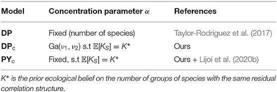
Table 1. Specification of concentration parameter α for the DP, DP_c, PY_c models.

2.3. Clustering Analysis

We summarize the posterior distribution of the clusters to obtain a clustering (i.e., partition of species) for each model DP, DP_c, and PY_c (the procedure is described in Supplementary Material, section 7). Notice that there is a difference between the posterior expected number of clusters and the number of clusters of the estimated clustering, obtained by the algorithm described in Supplementary Material (section 7) for posterior inference on partition space. The former describes the distribution of the number of clusters in Markov chain Monte Carlo (MCMC) samples (Robert and Casella, 2004), while the latter represents the number of clusters in the single partition that best represents the posterior distribution of the clusters in the MCMC samples. Generally, even if one has certain prior knowledge on the number of groups, it is possible that there is no information on the cluster composition. In our case study, we have a prior expected number of clusters and we also have a cluster composition. For this reason, we could also assess the composition of obtained cluster in-depth. To do so, we measured the distance between the clusters obtained by the models and the clusters we used as a prior belief. We used the adjusted Rand index (ARI) (Hubert and Arabie, 1985), which is the corrected for chance proportion of the number of agreements (species clustered similarly) in all possible pairs of species divided by the total number of all possible pairs. This value is between 0 and 1, where 1 corresponds to exactly the same cluster composition. Additionally, we checked how the choice of the prior number of groups affects the posterior distribution (sensitivity to the prior, Supplementary Material, section 8.3).

3. Case Study

3.1. Study Site and Species Information

We illustrated our methods with data on plant species in Bauges Natural Regional Park (France) available from the Alpine Botanical Conservatory (CBNA) and previously analyzed by Thuiller et al. (2018). We included as covariates the first two principal components of the environmental variables presented by Thuiller et al. (2018), including a quadratic term (using orthogonal polynomials to reduce correlation among the covariates). We considered presence-absence for the 111 most abundant species (present at least in 2% of sites) across the 1–139 plots. For details on the data processing steps (see Supplementary Material, section 1). We considered the 16 plant functional groups (PFGs) that were built in Thuiller et al. (2018). These PFGs have been obtained through hierarchical clustering, in order to build groups of species that have a similar functional role: they have a similar tolerance of abiotic conditions, dispersal abilities, resistance to disturbance (grazing and mowing), response to competition for light (whether they germinate and grow under specific light conditions), competitive effects (estimated by the height of the species) and demographic characteristics (life-form, longevity, age of maturity). We refer to Thuiller et al. (2018) for a complete description of PFGs and how they were classified. The number of these groups were used to specify the DP_c and PY_c priors, by fixing 𝔼[K_S] = 16. Note that the number of groups, but not their composition, was used for prior specification.

3.2. Implementation and Specification of the Models

We applied our DP_c and PY_c models together with the original DP model in dimension reduction with the default settings on the Bauges plant data. We fitted the models using Bayesian inference via MCMC using a Gibbs sampling scheme. For the original DP model, we used the R package GJAM (Taylor-Rodriguez et al., 2017). We implemented the DP_c and PY_c models in R by extending the original GJAM R package. In particular, we implemented an additional adaptive Metropolis–Hasting step (for DP_c) and the multi-step algorithm proposed by Lijoi et al. (2020b) to sample from PY_c (see details in Supplementary Material, section 6). Our code (an extension of the GJAM package) can be found at the first author's Github repository (https://github.com/dbystrova/GJAM_clust). The prior on the number of clusters was set using the number of plant functional groups (PFGs) as described above (see Supplementary Material, section 5 for the calibration method and for the importance of such step). For the sake of comparison, we used the same default non informative priors suggested by Clark et al. (2017) for all other parameters of the three models. Convergence was assessed through the calculation of Gelman–Rubin diagnostics (Gelman and Rubin, 1992) or visual inspection of the trace plots.

For the dimension reduction regime in GJAM model, the number of latent factors in the first step of dimension reduction needed to be specified. The number of latent factors was chosen using the deviance information criterion (DIC) (Spiegelhalter et al., 2002) (see details in Supplementary Material, section 2). Model fit was evaluated at the species level. Prediction performances were not the main objective of the paper, as we do not expect the residual covariance matrix to impact predictive mean values (Norberg et al., 2019; Wilkinson et al., 2019; Pichler and Hartig, 2020). However, we did check that the model fitted well the data both on training and test set. The dataset was randomly partitioned into a training and a testing dataset, using 70/30% ratio. We fitted models on the training dataset and then predicted species occurrences on the testing data, comparing the predicted and the actual occurrences, similarly to Norberg et al. (2019) and Wilkinson et al. (2019) (cross-validation is not a doable task due to the computational costs of the models). For each species, we measured the predictive performances by calculating the area under the receiver operating characteristic curve (AUC) on both training (AUC_in) and testing datasets (AUC_out).

3.3. Ecological Representation of the Clusters

We hypothesized that species within the same clusters might have similar functional strategies as measured by distance in trait space. We considered the following traits: Landolt nutrient indicator, Landolt light indicator, height (in the logarithmic scale), specific leaf area (SLA), leaf dry matter content (LDMC), leaf carbon concentration (LCC), and leaf nitrogen concentration (LNC) (Brun et al., 2019). All traits presented here were available for at least 70% of the species. For a more intuitive understanding, we assigned traits with a similar role in the community assembly process (Boulangeat et al., 2012) into four categories: competitive effect (height, SLA, LDMC, LCC, LNC), tolerance to abiotic and biotic conditions (Landolt nutrient indicator, Landolt light indicator), interaction via light resources (height, SLA, Landolt light indicator), and interaction via soil resources (LNC, Landolt nutrient indicator). Specifically, we calculated the following species-specific ratio for each species, each category of traits and each clustering method (including the PFGs) to measure whether species within the same cluster share a similar range of functional traits:

$\begin{array}{l}\text{Species grouped-trait ratio}\\ =\frac{{\text{mean(distance to other species)}}_{\text{within cluster}}}{{\text{mean(distance to other species)}}_{\text{all species}}}\end{array}$

In accordance with our hypothesis, we expected these distributions of species grouped-trait ratios to be close to zero, however not exactly zero, as exact zero would indicate the singleton clusters. This specifically indicates that the species were closer to within-cluster species than to species in the other clusters, thus fitted clusters could represent similar functional strategies. However, in our interpretation, we also penalized the clustering method when the number of singleton clusters increase as they do not serve the aim for clustering functionally similar species.

3.4. Results

3.4.1. Prediction Evaluation

Supplementary Table 2 provides the predictive performances (both in-sample and out-of-sample) of the models, that are all very similar across models. The data are well-explained (mean value of AUC_in is around 0.755), and the performances do not drop on the test dataset (AUC_out around 0.745).

3.4.2. Clustering Properties of the Models

The posterior distribution of the number of clusters of the DP model with a mean value of 35 was substantially lower than the prior mean of 56 (Supplementary Table 1, Figure 1). Larger variances for the DP_c and PY_c models reduced prior weight and thus posterior distributions remained closer to their prior mean of 16, yielding a posterior mean near 20 (Figure 1).

FIGURE 1

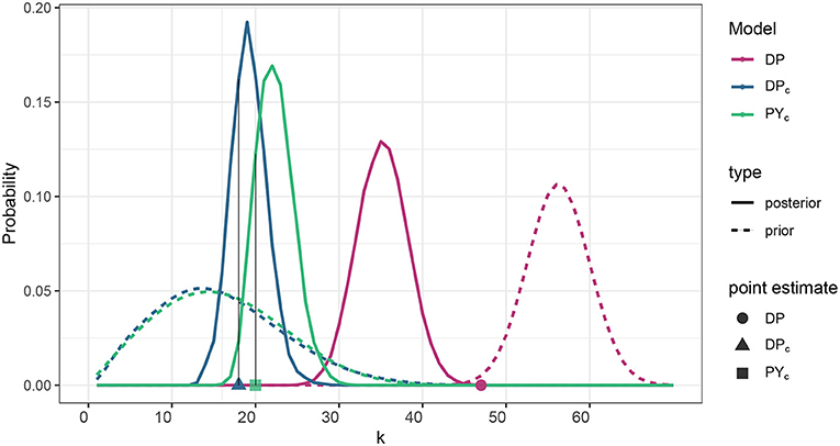
Figure 1. Prior distribution and posterior estimation of the number of clusters corresponding to DP, DP_c, PY_c models. For DP_c and PY_c models, prior distribution is specified such that 𝔼[K_S] matches the prior ecological knowledge (in our case it is the number of PFGs). Posterior estimation for all the models is represented by the posterior distribution of the number of clusters (solid lines) and the number of clusters of the posterior cluster estimate (points on x-axis). Refer to the clustering estimation procedure described in Supplementary Material, section S.7 for a pointer on why the size of the cluster estimate can be distant from the bulk of the posterior distribution.

Thus, the posterior cluster estimate from the DP model estimated more clusters than did the DP_c and PY_c models (18, and 20, respectively), which were closer to the number of PFG groups (16); see point estimates in Figure 1. Figure 2 provides the ARI as similarity measure between clusters estimated by each model and the PFGs. The posterior cluster estimates for all models are distant from the PFGs as the value of the ARI measure between each of the clusters and PFGs is close to zero. The DP is however more distant from PFGs than DP_c and PY_c. The DP_c and PY_c models yielded cluster estimates similar to one another (Figure 2). Pairwise similarities with a random partition in the Supplementary Material (see Supplementary Figure 5) show that PFGs are closer to the estimated clusters than a random partition.

FIGURE 2

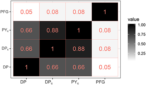
Figure 2. Pairwise ARI similarities between the PFGs and the clusters estimated by the models (DP, DP_c, PY_c).

We have tested sensitivity to prior specification for the PY_c and DP_c models, specifying prior at lower (8) and larger (56) values (Figure 3). PY_c model which has a larger variance for the prior distribution of the number of clusters, appeared to be less sensitive to prior specification than DP_c.

FIGURE 3

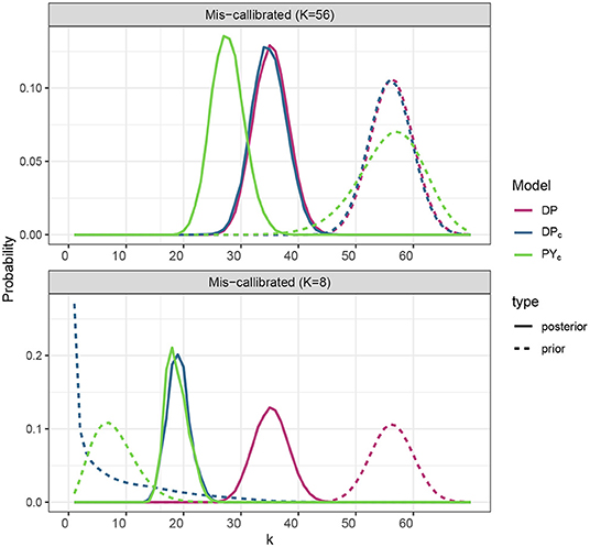
Figure 3. Prior and posterior distribution of the number of clusters for the models DP_c, PY_c corresponding to the different prior specification of the number of clusters, where prior expected number of clusters 𝔼[K_S] take values in {8, 56}.

3.4.2.1. Clusters Interpretation

The clusters estimated by DP_c and PY_c represent functional strategies (Figure 4), particularly for traits related to tolerance. The resulting clustering of the DP model contains many singleton clusters (i.e., clusters with one species), which have zero grouped-trait ratio, thus imply lower overall grouped-trait ratio for DP model (Figure 4). Supplementary Figures 7–9 show the residual covariance matrix inferred by the models.

FIGURE 4

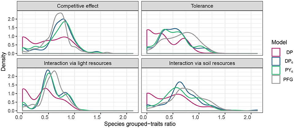
Figure 4. Distribution of species grouped-trait ratio for different trait categories and for all clustering methods. The reference curve is the distribution of species grouped-trait ratio of PFGs (DP,DP_c, PY_c).

4. Discussion

Understanding what are the main environmental drivers of species distributions and biodiversity is one of the main goad of ecology. This task requires to consider a large number of species with as a consequent high computational cost of the models employed, whose feasibility depends on dimension reduction and the inclusion of an expert-based prior knowledge. Here, we presented an extension of the dimension reduction approach for joint species distribution models proposed by Taylor-Rodriguez et al. (2017), by incorporating prior knowledge and by providing a more flexible clustering method. While reducing the dimension of the model, we provide a tool to create groups of species that share the same associations with respect to other species. For studies where a specific residual covariance structure is desirable our approach brings new flexibility to JSDMs. Our application shows a case where residual covariance is structured in agreement with functional traits, suggesting that these traits determine presence-absence beyond what is explained by the mean structure of the model.

4.1. Clustering Properties of the Models

The results of our case study confirm the importance of carefully choosing the prior in the DP model proposed by Taylor-Rodriguez et al. (2017). The DP specifies greater prior weight on the number of clusters than can be desirable in some applications. For this application where we specified a prior mean that was far from the posterior (i.e., using the default settings of Taylor-Rodriguez et al., 2017), the posterior distribution of the number of clusters of the DP model moved far from the prior, but without the full flexibility we offer here (Figure 1). Large prior variances on the DP_c and PY_c models make them less informative. In this application where we specified a prior mean close to the posterior, we found prior-posterior agreement.

By tuning the parameter N, the DP model would have also recovered the desired number of clusters. However, due its very peaky prior distribution (i.e., strong prior weight), it has less flexibility to move far from the prior when sample size is limited (sample size in our case, number of plots is n = 1, 139, number of species is S = 111). For this reasons we did not test for the ability of this model in the case study. Finally, the fact that the posterior distribution of the number of clusters of PY_c for different prior choices stay close, confirms that the prior on the number of clusters for the models (𝔼[K_S] = 16) is well-chosen.

4.2. The Importance of Prior Elicitation

Including prior knowledge is an appealing feature of Bayesian statistics, which is however often unused, or worse, misused (Banner et al., 2020). Expert-based prior knowledge on species interactions has always been available, and it is now getting more and more accessible (Maiorano et al., 2020). While co-occurrence networks should not be interpreted as interaction networks, we claim that this prior knowledge can help to separate the effect of the environment from the one of biotic interactions, to improve inference of interaction networks, but also to account for biotic interactions in predictive distribution models. In our case, prior knowledge does not concern particular species-specific interactions, but informs the model on the number of groups of species that share the same associations with other species. Although these associations should not be confounded with interactions, we suggest that our model DP_c is a first attempt to include prior information when building co-occurrence networks. Since time-series contain much more informations on biotic interactions than snapshot data, we could further extend our model to cluster the autoregressive coefficients of dynamic JSDMs (Ovaskainen et al., 2017a; Clark et al., 2020), in order to truly include a prior knowledge on the structure of the interaction network.

4.3. Clustering Species in JSDMs Framework

Thanks to new sampling techniques (e.g., eDNA, Taberlet et al., 2012), community data are becoming more and more available. Learning the structure of a co-occurrence network from data with a large number of species is particularly demanding, since for a given number of nodes S, there exists 2^S possible networks. Moreover, even in case a correct inference is possible, it is not an easy task to visualize, and then summarize and analyze a large network. Clustering species allows to zoom out from the species level, focusing on a broader scale, easier to model, visualize, and describe (Ohlmann et al., 2019). Indeed, our model both reduce the dimension of the problem and enable a better understanding of the ecosystem under study, showing how these clusters are strongly linked to functional traits. We emphasize that our method is conceptually different from applying a clustering method (e.g., hierarchical clustering) on the inferred residual correlation matrix, because in that case species in the same cluster do not exactly share the same residual associations and the dimensions of the model would not be reduced. Finally, we notice that since we cluster the residual correlation matrix, we do not filter out indirect associations (Harris, 2016; Popovic et al., 2019). To do so, our model should be extended to cluster the residual partial correlation matrix (i.e., the inverse of the residual correlation matrix) to truly represent a co-occurrence network, and not a network of marginal correlations (that represent both direct and indirect associations).

4.4. The Role of Functional Traits to Shape Community Assemblages

With our case study, we show how the proposed clustering methodology could facilitate the description and provide better insights of the residual covariance matrix. Firstly, while we acknowledge that such a residual covariance matrix should not be interpreted as a species interaction network, we believe that we can still attribute a certain ecological meaning to the residual associations between species. Indeed, species within the same inferred clusters share similar competitive abilities, similar tolerance level to abiotic and biotic conditions and interact in the same way even when we consider ecological processes at different levels such as interactions for light and soil resources (Figure 4). Moreover, species within the same clusters tend to be positively correlated (Supplementary Figures 8, 9). For example, with both clustering methods (DP_c and PY_c), we observed that Sorbus aria (i.e., mountainous tree) and Hieracium murorum form a cluster. The latter being a mountainous understory herbaceous species it needs the shade provided by the former: therefore, the two are positively correlated in the residual covariance matrix. Another example is given by five species (Lonicera xylosteum, Corylus avellana, Mercurialis perennis, Hedera helix, Fraxinus excelsior) from different life forms that are always grouped together with both clustering methods (DP_c and PY_c) for that they are all found mainly at forest edges and the herbaceous understory species, Mercurialis perennis, benefiting from the shade of the trees. In addition, the same cluster is negatively correlated with the big cluster no. 5 (built with PY_c method, Supplementary Figure 9) that is mainly grouping lowland to subalpine species that are shade-intolerant but can tolerate nutrient poor soils. In sum, the groups of species that we build represent those species that tend to co-occur together more than expected by the lens of observed environmental variables. Notice that this might also be an indication that species within the same clusters also happen to be in similar habitats, suggesting missing environmental variables. Notably, the fact that species within the same clusters tent to show similar values of the Landolt nutrient indicator suggests that soil properties might explain some of the residual correlations (Supplementary Figure 3).

Moreover, we believe that these results will also have practical advantages. The PFG building framework (Boulangeat et al., 2012) allows to group species according to their functional strategies in the aim of reducing the botanical complexity in dynamic vegetation models. As shown here, our models provide clusters that could represent similarity in tolerance to abiotic and biotic conditions and their competitive ability at least as much as PFGs. Hence, the obtained clusters in our case can be considered as a valuable alternative to the PFG building framework, that requires the availability of many functional traits for most species.

Despite these improvements and advantages, we also acknowledge some possible pitfalls. Notably, missing covariates have always the potential to drive the patterns in the residual covariance matrix. The fact that our clusters performed well in representing the traits related to tolerance to abiotic conditions might be an indication of such a problem. Among these traits, Landolt nutrient indicator represents soil nutritive requirements of plants and was quite well represented by the clusters (Supplementary Figure 3). Having in mind that we were not able to include soil data among the covariates for this case study due to data availability, it is possible that the residual co-occurrence patterns are also driven by the soil properties. Another way forward in the framework would also be including habitat and soil information as covariates to further investigate if we can retrieve different patterns in the residual covariance matrix that are more directly related to biotic interactions.

5. Conclusion

We propose a statistical framework that allows an additional but ecologically meaningful dimension reduction of joint species distribution models and includes prior knowledge in the residual covariance matrix, providing a tool to infer clusters of species that share the same residual associations with respect to other species. The case study shows that the obtained clusters of species are ecologically meaningful, and correlated with functional traits. Therefore, our model can also be seen as an alternative way to build functional groups without having to measure all necessary traits.

Data Availability Statement

The datasets analyzed for this study can be found at the first author's Github repository (https://github.com/dbystrova/GJAMclust).

Author Contributions

WT, JA, DB, and GP conceived the idea. AG, JA, DB, and GP developed statistical methods. DB and GP implemented the methods in R. DB, GP, and BB analyzed the data for the case study. DB, GP, BB, JA, JC, and WT wrote the first draft of the manuscript. All authors contributed substantially to the revisions.

Funding

DB, GP, and WT were supported by the GAMBAS project funded by the French National Research Agency (ANR-18-CE02-0025). JA was supported by the Grenoble Alpes Data Institute, funded by the French National Research Agency (ANR-15-IDEX-02). JC and WT also acknowledged support from the Programme d'Investissement d'Avenir under project FORBIC (18-MPGA-0004). This work also received funding from the ERA-Net BiodivERsA - Belmont Forum, with the national funder Agence National pour la Recherche (FutureWeb: ANR-18-EBI4–0009) to WT and the National Science Foundation (NSF grant No 1854976) to JC. This work has been partially supported by MIAI @ Grenoble Alpes (ANR-19-P3IA-0003).

Conflict of Interest

The authors declare that the research was conducted in the absence of any commercial or financial relationships that could be construed as a potential conflict of interest.

Supplementary Material

The Supplementary Material for this article can be found online at: https://www.frontiersin.org/articles/10.3389/fevo.2021.601384/full#supplementary-material

References

Banner, K. M., Irvine, K. M., and Rodhouse, T. (2020). The Use of bayesian priors in ecology: the good, the bad, and the not great. Methods Ecol. Evol. 11 882–889. doi: 10.1111/2041-210X.13407

CrossRef Full Text | Google Scholar

Boulangeat, I., Philippe, P., Abdulhak, S., Douzet, R., Garraud, L., Lavergne, S., et al. (2012). Improving plant functional groups for dynamic models of biodiversity: at the crossroads between functional and community ecology. Glob. Change Biol. 18, 3464–3475. doi: 10.1111/j.1365-2486.2012.02783.x

PubMed Abstract | CrossRef Full Text | Google Scholar

Brun, P., Zimmermann, N. E., Graham, C. H., Lavergne, S., Pellissier, L., Münkemüller, T., et al. (2019). The productivity-biodiversity relationship varies across diversity dimensions. Nat. Commun. 10, 1–11. doi: 10.1038/s41467-019-13678-1

PubMed Abstract | CrossRef Full Text | Google Scholar

Bystrova, D., Arbel, J., King, G. K. K., and Deslandes, F. (2021). “Approximating the clusters' prior distribution in Bayesian nonparametric models,” in Third Symposium on Advances in Approximate Bayesian Inference. Virtual Event.

Google Scholar

Calabrese, J. M., Certain, G., Kraan, C., and Dormann, C. F. (2014). Stacking species distribution models and adjusting bias by linking them to macroecological models. Glob. Ecol. Biogeogr. 23, 99–112. doi: 10.1111/geb.12102

CrossRef Full Text | Google Scholar

Chen, D., Xue, Y., and Gomes, C. (2018). “End-to-end learning for the deep multivariate probit model,” in Proceedings of Machine Learning Research, Vol. 80 (Stockholm: PMLR), 932–941.

Google Scholar

Chib, S., and Greenberg, E. (1998). Analysis of multivariate probit models. Biometrika 85, 347–361. doi: 10.1093/biomet/85.2.347

CrossRef Full Text | Google Scholar

Chiquet, J., Robin, S., and Mariadassou, M. (2019). “Variational inference for sparse network reconstruction from count data,” in International Conference on Machine Learning (Long Beach), 1162–1171.

Google Scholar

Clark, J. S., Nemergut, D., Seyednasrollah, B., Turner, P. J., and Zhang, S. (2017). Generalized joint attribute modeling for biodiversity analysis: median-zero, multivariate, multifarious data. Ecol. Monogr. 87, 34–56. doi: 10.1002/ecm.1241

CrossRef Full Text | Google Scholar

Clark, J. S., Scher, C. L., and Swift, M. (2020). The emergent interactions that govern biodiversity change. Proc. Natl. Acad. Sci. U.S.A. 117, 17074–17083. doi: 10.1073/pnas.2003852117

PubMed Abstract | CrossRef Full Text | Google Scholar

De Blasi, P., Favaro, S., Lijoi, A., Mena, R. H., Prünster, I., and Ruggiero, M. (2015). Are Gibbs-type priors the most natural generalization of the Dirichlet process? IEEE Trans. Pattern Anal. Mach. Intell. 37, 212–229. doi: 10.1109/TPAMI.2013.217

PubMed Abstract | CrossRef Full Text | Google Scholar

Dormann, C. F., Bobrowski, M., Dehling, D. M., Harris, D. J., Hartig, F., Lischke, H., et al. (2018). Biotic interactions in species distribution modelling: 10 questions to guide interpretation and avoid false conclusions. Glob. Ecol. Biogeogr. 27, 1004–1016. doi: 10.1111/geb.12759

CrossRef Full Text | Google Scholar

Elith, J., and Leathwick, J. R. (2009). Species distribution models: ecological explanation and prediction across space and time. Annu. Rev. Ecol. Evol. Syst. 40, 677–697. doi: 10.1146/annurev.ecolsys.110308.120159

CrossRef Full Text | Google Scholar

Ferguson, T. (1973). A Bayesian analysis of some nonparametric problems. Ann. Stat. 1, 209–230. doi: 10.1214/aos/1176342360

CrossRef Full Text | Google Scholar

Ferrier, S., and Guisan, A. (2006). Spatial modelling of biodiversity at the community level. J. Appl. Ecol. 43, 393–404. doi: 10.1111/j.1365-2664.2006.01149.x

CrossRef Full Text | Google Scholar

Gelman, A., Carlin, J. B., Stern, H. S., and Rubin, D. B. (2004). Bayesian Data Analysis. New York, NY: CRC Press. doi: 10.1201/b16018

CrossRef Full Text | Google Scholar

Gelman, A., and Rubin, D. B. (1992). Inference from iterative simulation using multiple sequences. Stat. Sci. 7, 457–472. doi: 10.1214/ss/1177011136

CrossRef Full Text | Google Scholar

Geweke, J. F., and Singleton, K. J. (1980). Interpreting the likelihood ratio statistic in factor models when sample size is small. J. Am. Stat. Assoc. 75, 133–137. doi: 10.1080/01621459.1980.10477442

CrossRef Full Text | Google Scholar

Guisan, A., and Thuiller, W. (2005). Predicting species distribution: offering more than simple habitat models. Ecol. Lett. 8, 993–1009. doi: 10.1111/j.1461-0248.2005.00792.x

CrossRef Full Text | Google Scholar

Guisan, A., Thuiller, W., and Zimmermann, N. E. (2017). Habitat Suitability and Distribution Models: With Applications in R. Cambridge, MA: Cambridge University Press. doi: 10.1017/9781139028271

CrossRef Full Text | Google Scholar

Harris, D. J. (2015). Generating realistic assemblages with a joint species distribution model. Methods Ecol. Evol. 6, 465–473. doi: 10.1111/2041-210X.12332

CrossRef Full Text | Google Scholar

Harris, D. J. (2016). Inferring species interactions from co-occurrence data with Markov networks. Ecology 97, 3308–3314. doi: 10.1002/ecy.1605

PubMed Abstract | CrossRef Full Text | Google Scholar

Hubert, L., and Arabie, P. (1985). Comparing partitions. J. Classif. 2, 193–218. doi: 10.1007/BF01908075

CrossRef Full Text | Google Scholar

Hui, F. K. (2016). Bayesian ordination and regression analysis of multivariate abundance data in R. Methods Ecol. Evol. 7, 744–750. doi: 10.1111/2041-210X.12514

CrossRef Full Text | Google Scholar

Lee, C., and Wilkinson, D. J. (2019). A review of stochastic block models and extensions for graph clustering. Appl. Netw. Sci. 4:122. doi: 10.1007/s41109-019-0232-2

CrossRef Full Text | Google Scholar

Lijoi, A., Prünster, I., and Rigon, T. (2020a). Finite-Dimensional Discrete Random Structures and Bayesian Clustering. Tech. rep. Collegio Carlo Alberto.

Google Scholar

Lijoi, A., Prünster, I., and Rigon, T. (2020b). The Pitman-Yor multinomial process for mixture modeling. Biometrika 107, 891–906. doi: 10.1093/biomet/asaa030

CrossRef Full Text | Google Scholar

Maiorano, L., Montemaggiori, A., Ficetola, G. F., O'Connor, L., and Thuiller, W. (2020). TETRA-EU 1.0: A species-level trophic metaweb of European tetrapods. Glob. Ecol. Biogeogr. 29, 1452–1457. doi: 10.1111/geb.13138

CrossRef Full Text | Google Scholar

Merow, C., Smith, M. J., Edwards, T. C. Jr, Guisan, A., McMahon, S. M., Normand, S., et al. (2014). What do we gain from simplicity versus complexity in species distribution models? Ecography 37, 1267–1281. doi: 10.1111/ecog.00845

CrossRef Full Text | Google Scholar

Moscone, F., Tosetti, E., and Vinciotti, V. (2017). Sparse estimation of huge networks with a block-wise structure. Econ. J. 20, S61–S85. doi: 10.1111/ectj.12078

CrossRef Full Text | Google Scholar

Muliere, P., and Secchi, P. (2003). Weak convergence of a Dirichlet-multinomial process. Georg. Math. J. 10, 319–324. doi: 10.1515/GMJ.2003.319

CrossRef Full Text | Google Scholar

Norberg, A., Abrego, N., Blanchet, F. G., Adler, F. R., Anderson, B. J., Anttila, J., et al. (2019). A comprehensive evaluation of predictive performance of 33 species distribution models at species and community levels. Ecol. Monogr. 89, 834–848. doi: 10.1002/ecm.1370

CrossRef Full Text | Google Scholar

O'Connor, L. M., Pollock, L. J., Braga, J., Ficetola, G. F., Maiorano, L., Martinez-Almoyna, C., et al. (2020). Unveiling the food webs of tetrapods across Europe through the prism of the Eltonian niche. J. Biogeogr. 47, 181–192. doi: 10.1111/jbi.13773

CrossRef Full Text | Google Scholar

Ohlmann, M., Miele, V., Dray, S., Chalmandrier, L., O'Connor, L., and Thuiller, W. (2019). Diversity indices for ecological networks: a unifying framework using hill numbers. Ecol. Lett. 22, 737–747. doi: 10.1111/ele.13221

PubMed Abstract | CrossRef Full Text | Google Scholar

Ovaskainen, O., and Abrego, N. (2020). Joint Species Distribution Modelling: With Applications in R. Cambridge, MA: Cambridge University Press.

Google Scholar

Ovaskainen, O., Abrego, N., Halme, P., and Dunson, D. (2016). Using latent variable models to identify large networks of species-to-species associations at different spatial scales. Methods Ecol. Evol. 7, 549–555. doi: 10.1111/2041-210X.12501

CrossRef Full Text | Google Scholar

Ovaskainen, O., Tikhonov, G., Dunson, D., Grøtan, V., Engen, S., Saether, B.-E., et al. (2017a). How are species interactions structured in species-rich communities? A new method for analysing time-series data. Proc. R. Soc. B Biol. Sci. 284:20170768. doi: 10.1098/rspb.2017.0768

PubMed Abstract | CrossRef Full Text | Google Scholar

Ovaskainen, O., Tikhonov, G., Norberg, A., Guillaume Blanchet, F., Duan, L., Dunson, D., et al. (2017b). How to make more out of community data? A conceptual framework and its implementation as models and software. Ecol. Lett. 20, 561–576. doi: 10.1111/ele.12757

PubMed Abstract | CrossRef Full Text | Google Scholar

Pichler, M., and Hartig, F. (2020). A new method for faster and more accurate inference of species associations from novel community data. arXiv preprint arXiv:2003.05331.

Google Scholar

Pitman, J. (2006). Combinatorial Stochastic Processes: Ecole d'Eté de Probabilités de Saint-Flour XXXII-2002. Berlin; Heidelberg: Springer.

Google Scholar

Pitman, J., and Yor, M. (1997). The two-parameter poisson-dirichlet distribution derived from a stable subordinator. Ann. Probabil. 855–900. doi: 10.1214/aop/1024404422

CrossRef Full Text | Google Scholar

Poggiato, G., Münkemüller, T., Bystrova, D., Arbel, J., Clark, J., and Thuiller, W. (2021). On the interpretations of joint modelling in community ecology. Trends Ecol. Evol. doi: 10.1016/j.tree.2021.01.002. [Epub ahead of print].

PubMed Abstract | CrossRef Full Text | Google Scholar

Pollock, L. J., Tingley, R., Morris, W. K., Golding, N., O'Hara, R. B., Parris, K. M., et al. (2014). Understanding co-occurrence by modelling species simultaneously with a Joint Species Distribution Model. Methods Ecol. Evol. 5, 397–406. doi: 10.1111/2041-210X.12180

CrossRef Full Text | Google Scholar

Popovic, G. C., Warton, D. I., Thomson, F. J., Hui, F. K., and Moles, A. T. (2019). Untangling direct species associations from indirect mediator species effects with graphical models. Methods Ecol. Evol. 10, 1571–1583. doi: 10.1111/2041-210X.13247

CrossRef Full Text | Google Scholar

Robert, C. P., and Casella, G. (2004). Monte Carlo Statistical Methods. New York, NY: Springer-Verlag. doi: 10.1007/978-1-4757-4145-2

CrossRef Full Text | Google Scholar

Spiegelhalter, D. J., Best, N. G., Carlin, B. P., and Van Der Linde, A. (2002). Bayesian measures of model complexity and fit. J. R. Stat. Soc. Ser. B 64, 583–639. doi: 10.1111/1467-9868.00353

CrossRef Full Text | Google Scholar

Taberlet, P., Coissac, E., Hajibabaei, M., and Rieseberg, L. H. (2012). Environmental DNA. Mol. Ecol. 21, 1789–1793. doi: 10.1111/j.1365-294X.2012.05542.x

CrossRef Full Text | Google Scholar

Taylor-Rodriguez, D., Kaufeld, K., Schliep, E. M., Clark, J. S., and Gelfand, A. E. (2017). Joint species distribution modeling: dimension reduction using Dirichlet processes. Bayesian Anal. 12, 939–967. doi: 10.1214/16-BA1031

PubMed Abstract | CrossRef Full Text | Google Scholar

Thuiller, W., Guéguen, M., Bison, M., Duparc, A., Garel, M., Loison, A., et al. (2018). Combining point-process and landscape vegetation models to predict large herbivore distributions in space and time–A case study of Rupicapra rupicapra. Divers. Distrib. 24, 352–362. doi: 10.1111/ddi.12684

CrossRef Full Text | Google Scholar

Thuiller, W., Münkemüller, T., Lavergne, S., Mouillot, D., Mouquet, N., Schiffers, K., et al. (2013). A road map for integrating eco-evolutionary processes into biodiversity models. Ecol. Lett. 16, 94–105. doi: 10.1111/ele.12104

PubMed Abstract | CrossRef Full Text | Google Scholar

Vanhatalo, J., Hartmann, M., and Veneranta, L. (2020). Additive multivariate gaussian processes for joint species distribution modeling with heterogeneous data. Bayesian Anal. 15, 415–447. doi: 10.1214/19-BA1158

CrossRef Full Text | Google Scholar

Warton, D. I., Blanchet, F. G., O'Hara, R. B., Ovaskainen, O., Taskinen, S., Walker, S. C., et al. (2015). So many variables: joint modeling in community ecology. Trends Ecol. Evol. 30, 766–779. doi: 10.1016/j.tree.2015.09.007

PubMed Abstract | CrossRef Full Text | Google Scholar

Wilkinson, D. P., Golding, N., Guillera-Arroita, G., Tingley, R., and McCarthy, M. A. (2019). RA comparison of joint species distribution models for presence-absence data. Methods Ecol. Evol. 10, 198–211. doi: 10.1111/2041-210X.13106

CrossRef Full Text | Google Scholar