
95% of researchers rate our articles as excellent or good
Learn more about the work of our research integrity team to safeguard the quality of each article we publish.
Find out more
ORIGINAL RESEARCH article
Front. Ecol. Evol. , 21 March 2018
Sec. Marine Ecosystem Ecology
Volume 6 - 2018 | https://doi.org/10.3389/fevo.2018.00023
This article is part of the Research Topic Complexity in Marine Systems: Developing a pragmatic approach to understanding and managing their emergent features View all 6 articles
The distribution and population dynamics of zooplankton are affected by the interplay between currents, behavior, and selective growth, mortality, and reproduction. Here, we present an individual based model for a copepod where life-history and behavioral traits are adapted using a genetic algorithm approach. The objectives were to investigate the importance of spatial and inter-annual variability in biophysical forcing and different predator densities on the adaptation of emergent life history traits in a copepod. The results show that in simulations with adaptation, the populations remained viable (positive population growth) within the study area over 100-year simulation whereas without adaptation populations were unviable. In one dimensional simulations with fixed spatial position there were small differences between replicate simulations. Inter-annual variability in forcing resulted in increased difference in fitness between years. Simulations with spatial-, but without inter-annual variability in forcing produced large differences in the geographic distribution, fitness, and life history strategies between replicate simulations. In simulations with both spatial and inter-annual variability the replicates had rather small variability in traits. Increased predator density lead to increased day depth and avoidance of the lit upper waters. The model can be used for a range of different applications such as studying individual and population responses to environmental changes including climate change as well as to yield robust behavioral strategies for use in fully coupled end to end ecosystem models.
The distribution and population dynamics of zooplankton are affected by the interplay between currents, behavior, and selective growth, mortality, and reproduction. Zooplankton can respond to a range of environmental factors including predators, prey, and physical factors such as temperature (Bollens and Frost, 1989; Carlotti et al., 2000; Fiksen, 2000). Most meso-zooplankton species are coupled to phytoplankton dynamics and change growth and development rates in response to changes in food availability (e.g., Campbell et al., 2001). Predation is generally important in shaping life histories of organisms (Roff, 1992; Stearns, 1992). The effects can generally be divided into lethal and non-lethal components where that latter are features resulting from the predators “scaring” prey to stay away from otherwise preferred habitats (Creel and Christianson, 2008), the so called ecology of fear (Brown et al., 1999). Furthermore organisms inhabiting the sea have the inherent problem of upholding life cycle closure due to the advective and diffusive forces that continuously act to disperse populations (Sinclair, 1988; Eiane et al., 1998). Spatially explicit individual based models can be valuable for investigating the interplay between these productive, selective and dispersive factors on the spatial-temporal dynamics of zooplankton.
The copepod Calanus finmarchicus is the dominant species of the meso zooplankton in the Norwegian Sea (Melle et al., 2004) and is treated as our model species in this work. The species is largely herbivorous and constitutes an important link between the phytoplankton and the higher trophic levels in the North Atlantic food web (Aksnes and Blindheim, 1996; Melle et al., 2004). The life cycle of C. finmarchicus consists of overwintering at depth mainly as copepodite stages 4 (C4) or 5 (C5), ascent toward the surface during early spring, maturation, and subsequent commencement of egg production prior to and during the spring phytoplankton bloom (Marshall and Orr, 1955; Hirche, 1996b). The new generation remains in the upper waters during summer and may mature and reproduce within the season or build up fat reserves and descend to overwintering at stage C4 or C5 (Hirche, 1996a). The spring bloom is important for the timing of ascent from diapause (Hirche, 1996a), and Kaartvedt (2000) argues that predation from planktivorous fish is a key driver in the timing of the descent to overwintering. The timing of ascent and descent is a trade-off between growth, survival, and reproduction.
Plankton need to utilize the vertical and horizontal differentiation in the current pattern to close their life cycle. This is particularly challenging in areas of strong prevailing currents. Using drift trajectory data from RAFOS floats drifting at 800 m it has been estimated that C. finmarchicus are displaced over 300 km during the overwintering period in the Norwegian Sea (Søiland and Huse, 2012). Bryant et al. (1998) studied the drift pattern resulting from different depth distributions that mimicked the vertical distribution of C. finmarchicus. They found that some areas of the Norwegian Sea such as the Norwegian Basin and the area around the Faroese Islands could retain particles over more than 10 years. Torgersen and Huse (2005) found similar results in an individual based model taking into account growth, survival and reproduction as well as different seasonal vertical migration behaviors. The model results showed that the vertical migration behaviors with the highest advective loss rates were those that ascended early and descended late to diapause.
Due to the spatial heterogeneity and temporal variability of marine ecosystems spatially explicit models are sensitive to how phenology, life history traits and behavior are modeled. Parameterization of these traits in ecosystem models by using observations and experiments is challenging and costly. A different approach is instead to keep these behavioral traits free to evolve during the simulations using a genetic algorithm (Holland, 1975). This concept involves equipping individuals with “genes” and adapting these by simulating evolution by natural selection over many generations (Huse and Giske, 1998; Huse et al., 1999). In many ways, this can be considered parallel to the “spin up time” used in ocean circulation models. We developed an individual based model for a copepod based on previous model studies that include growth, mortality, and reproduction as well as adaptive traits for controlling phenology and the interaction with the environment. Fiksen (2000) developed a 1D IBM for C. finmarchicus with three traits determining the time for ascent from diapause, the day for preparing for overwintering and the relative fat content to be obtained before descending to diapause. We use the same traits as Fiksen (2000), add three traits related to controlling vertical distribution of the copepod and implement the copepod model in a 3D biophysical ocean model that generates temperature, advection and phytoplankton fields. The objectives are to use the adaptive IBM to investigate the effects of spatial and inter-annual variability in biophysical forcing and predator density on the adaptation of life history traits, retention and fitness of a copepod.
The model description is set in accordance with the protocol for describing IBMs proposed by Grimm et al. (2006). This entails an initial model overview in the subsequent paragraphs followed by a more detailed description of the model components under Submodels.
The model is a 3D individual-based model taking into account life history, behavior, growth, mortality, and reproduction of a copepod resembling loosely C. finmarchicus. Adaptive traits evolved using a genetic algorithm approach (Huse, 2005; Samuelsen et al., 2009) control the interaction with the environment. The entire life cycle of copepods and the main life history features and vertical movement are emergent properties resulting from many generations of evolution using a genetic algorithm (Figure 1). The purpose of the modeling is to improve understanding of the interplay between behavioral and life history trade-offs in relation to fitness, population dynamics and environmental variability in space and time. The model area is the Northeast Atlantic. Seven simulations were performed (Table 1), for a time period of 100 years. First two simulations (1 and 2) were performed without any spatial variability to study local adaptation with and without inter-annual variability in the biophysical forcing (currents, temperature, phytoplankton). The rest of the simulations had spatial variability in biophysical forcing. Two simulations (3 and 4) without inter-annual variability were performed, with and without selection to illustrate the effect of selection. Then a simulation (5) was performed where the years 1981–2004 were repeated sequentially during the adaptation process to study the effect of inter-annual variability. Finally, we investigate how differences in predation pressure affect the evolved strategies by varying the predation level by fish and tactile predators (6 and 7). For each simulation 4 replicate runs were made. This was done due to the reliance on stochastic processes and initialization where individuals differ with regards to initial position, composition of the strategy vectors, the sequence of mutations and movement diffusion. Since the simulated adaptation process depends on number of individuals in the population and is generally faster in smaller populations, four replicates of each simulation were made rather than one simulation with a four times greater number of individuals. For some of the result presentation, the output from the best replicate rather than average of the replicates is shown. This was done to maintain potential dependencies between the evolved traits. The “best” replicate is defined as having the highest average fitness (R0) for the last 30 years.
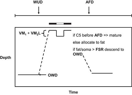
Figure 1. The conceptual framework of the life history traits of the copepod IBM. The strategy variables, whose values are evolved during the spin up simulation, are given in bold. OWD is the overwintering depth, WUD is the date at which the overwintering C5 starts ascent toward the surface, VM1 and VM2L gives the deepening of the copepod during day as a function of their length, AFD is the date after which an individual becoming C5 will prepare for overwintering, whereas before this date the individual will mature and reproduce in the same season, FSR gives the fat to soma ratio at which a C5 will descend to the OWD for overwintering in diapause.
The model comprises individuals and their environment. The attribute vector (Chambers, 1993) of individuals consists of 13 different states including their stage, internal number, weight, fat level, age, depth (Table 2). The strategy vector (SV) (Huse et al., 1999), which is evolved, contains all the life history and behavioral strategies of individuals and comprises five behavioral and life history traits. Each individual has a strategy vector that consists of:
The life history traits include the date for ascent from overwintering to the surface (WUD), the day for initiating fat allocation (AFD) in copepodite stage 5 (C5), fat/soma ratio needed before descending to overwintering (FSR), overwintering depth (OWD), and two genes (VM1 and VM2) that determine the day depth (DD) of non-overwintering copepodites (Figure 1). VM2 is multiplied by the size of the copepodite so that for values >0, there will be size dependent vertical migration. In the results reporting here were refer to the day depth, which is the resulting “phenotype” of WM1 and WM2 which are rather difficult to interpret. The three former traits (WUD, AFD, FSR) were presented by Fiksen (2000), while the latter three are introduced here. Even though the individual-based structure is appealing, it is impossible to simulate copepod population dynamics on a truly individual basis due to the great abundances involved, and the copepod is therefore simulated using the super-individual approach (Scheffer et al., 1995). A super-individual represents many identical individuals and the number of such identical siblings is an attribute of the super-individual (Table 2).
The processes governing the individuals are growth, mortality, movement, and reproduction. The simulated copepod goes through 13 different stages including an egg stage, six nauplia stages, five copepodite stages, and an adult stage. It is not assumed to commence feeding until the third nauplia stage (N3), and for stages below this, stage longevity was calculated as a function of temperature (Carlotti and Wolf, 1998). For stages N3 and above, growth is calculated as a function of phytoplankton density, temperature and size using a bioenergetics model (Carlotti and Wolf, 1998). The copepod is assumed to change stage when a stage specific critical weight is achieved. Thus, we did not utilize flexible critical weights. For the egg and nauplia stages, mortality consists of unspecified causes (taken from Ohman et al., 2004) and tactile predation. For the copepodite and adult stages mortality is attributed to predation from pelagic fish (herring, blue whiting, and mackerel), mesopelagic fish and tactile predators, starvation when the weight goes below the critical weight, and exhaustion if more than 800 eggs have been spawned. For individuals in diapause, no vertical movement is calculated, but for other individuals, movement is calculated either as a function of turbulence and sinking (stages < N3) or by adapted rules. A sex ratio of 50% is assumed, and males are removed from the population after one spawning event. Reproduction of adults can take place when their weight is above a threshold value and they have attained enough fat reserves to spawn a batch of eggs (Table 3). Spawning can only take place within the upper mixed layer (Table 3). If these conditions are met, the individual produces a new super-individual offspring whose internal number is a function of the batch size multiplied by the internal number of the mother. During reproduction, strategy vectors are passed on from parent to offspring.
The time step of the model is 1 h, simulated on a day-to-day basis over the entire year repeated a 100 times to evolve robust life history and behavioral traits (Table 2). Fat is allocated to structural growth for immature individuals, but mature individuals and C5s preparing for overwintering allocate their surplus energy into fat storage. During times of negative growth, the stored fat is depleted before the structural weight is reduced.
Most of the features of the model are emergent properties including the individual traits, mortality, growth, reproduction, and spatial dynamics.
The six life history traits are adapted and can be used to improve the fitness of individuals.
During the year super individuals grow, survive and may reproduce. At the end of the year the product of the internal number and the weight of each super individual is calculated. At the start of each year, a fixed number of super individuals are then drawn randomly from the previous year's population and the probability of being chosen is proportional to the product of the internal number and the weight.
Individuals are assumed to be able to sense the chlorophyll density and find the location of the depth with the highest chlorophyll density, they are also able to separate between day and night. They are also assumed to know which days are their inherited wake up and allocation to fat days, respectively.
Individuals interact indirectly through random cross over in the strategy vectors during reproduction.
There is random initiation of the strategy variables within bounds as defined below. In simulations with spatial variability the geographical locations of individuals is initiated stochastically given that the bottom depth is >100 m. Mutations and movement of egg-N2 are stochastic. There is a random walk component in the movement of super individuals to represent sub grid “diffusion” processes.
The individuals are super-individuals that each represents one or more identical individuals.
The model is initiated on January 1 with 500 super-individuals. The super-individuals are initiated as overwintering C5 at OWD or shallower if limited by bottom depth, at randomly chosen positions throughout the domain in areas where the bottom depth is >100 m (Figure 2). The valid grid cells have an equal probability of being chosen. The weight of individuals is 120 μg C and they have a fat reserve of 100 μg C (Carlotti and Wolf, 1998). The life history and behavioral traits are initiated randomly within given boundaries. Test runs were used to determine that the end solutions were not found outside the initiation ranges. The strategy vectors were initiated randomly within the ranges: WUD [15, 60], FSR [0.4, 0.8], AFD [100, 160], OWD [500, 1,000], VM1 [20, 60], VM2 [1,500, 4,500] for 500 individuals.
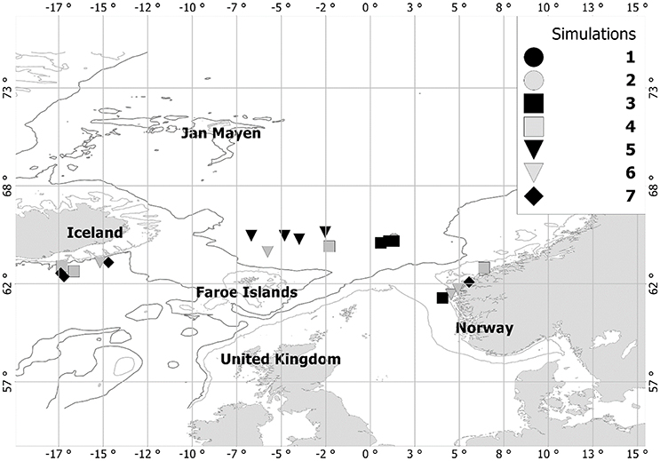
Figure 2. The average center of mass at the end of the year in the 30 last years in all four replicates of the simulations. The contours give the 200 and 500 m depth. Note that simulation 1 and 2 are in the same location centrally in the Norwegian Sea, hidden behind the two black squares (simulation 3).
Input data on light, currents, temperature, and phytoplankton biomass were taken from a model system involving the Regional Ocean Model System (ROMS) (Haidvogel et al., 2000) and the NORWECOM phytoplankton model, initially presented by Aksnes et al. (1995) and further developed by Skogen et al. (2007). Three day fields were interpolated linearly to daily values. The model domain is the Nordic Seas (56 to 82 N and 30 E to 30W, Figure 2). Each square is 1/3 longitude and 1/6 latitude which gives an approximate resolution of 20 km, and the total grid size was 181 by 153 squares. The NORWECOM model was run on a different grid as described in Skogen et al. (2007), and the results were transferred to the present grid as done previously (Utne and Huse, 2012; Utne et al., 2012b). Hourly surface light was generated from a model giving hourly sun height above the horizon (Skartveit and Olseth, 1988). The visual predators that include mesopelagic and pelagic fish were assumed to be distributed homogeneously in the upper 500 m and the tactile predators were assumed to be distributed in the upper 1,000 m.
The adaptive traits are implemented on a strategy vector Si (Equation 1) (Huse, 2001; Huse et al., 2002). A genetic algorithm (GA, Holland, 1975) is then used to optimize the strategy vector. The GA is a computational method that applies Darwin's principle of evolution by natural selection to search for optimal solutions to complex problems. The population of individuals is adapted by repeated testing, selection and reproduction. Instead of using maximization of a utility measure, we used emergent fitness to evolve the strategy vectors (Mitchell and Forrest, 1995; Huse, 1998; Strand et al., 2002). This concept involves simulating survival of the fittest over hundreds of generations, and considering the strategies dominating at the end to be those best adapted to the simulated environment. Only individuals that fulfill certain criteria can reproduce (see below). The selection scheme is inspired by the way natural selection works in nature. By repeating the procedure over and over, the population will consist of increasingly fit members. There is an inherent problem in individual based population models such as the present one in that the number of individuals may grow very large and thus increase computing time substantially. Since there was no density dependent feedback on the food resource, we implemented a direct density regulation. At the end of each year a fixed number of super individuals were selected from the population and passed on to the next year. This was done stochastically using Monte Carlo simulation and the probability for an individual being passed on to the next year was proportional to the product of its weight (structural + fat) and internal number which is the number of individuals represented by a super-individual (Scheffer et al., 1995). In this manner, a fixed number of 500 super individuals with a fixed internal number were initiated on each January 1. The density regulation will thus have less effect on the selection of individuals and their strategies than if density regulation was to be imposed for example on the food availability during the feeding season. The density regulation takes place during a time when the copepod is in diapause, so the start of January is an ideal timing of this regulating and does not interfere with any of its activities. The net reproductive rate R0 defined as the sum of the product of survival probability times the number of offspring produced is often used as a fitness proxy (e.g., Giske et al., 1993). Since R0 is closely related to our selection criteria we used it to report and contrast the results in different simulations.
Vertical position was updated at each hourly time step. During the egg and nauplia stages, individuals were restricted to stay in the upper 40 m. At each time step the vertical position was changed randomly by ±1 m, to mimic vertical diffusion in the upper mixed layer. During diapause, copepodites were assumed to stay at the overwintering depth (OWD) given by the strategy vector (Equation 1). Non-diapausing copepodites (stages 1 to adults) were assumed to stay at the chlorophyll maximum during the night hours. The day depth (DD) of copepodites (stages 1 to adults) was calculated as a function of the traits (Equation 1) and individual length (L) to allow for size dependent vertical distribution:
During ascent from and descent to overwintering the copepodites moved by a speed of 1 m h−1.
The feeding and growth model was adapted from Carlotti and Wolf (1998). It was assumed here that the copepod feed solely on phytoplankton, even though calanoid copepods, are known to be omnivorous and can also feed on microzooplankton. Ingestion (I) was calculated as a function of temperature, size, and phytoplankton level:
where Imax, Q10, a, b1, and b2 are constants (Table 3), phy is the phytoplankton concentration, W is the structural weight, and T is the temperature. The functional response parameters (b1 and b2) were scaled to resemble the relationships presented in Campbell et al. (2001). Respiration was calculated as a function of structural weight, temperature, and ingestion:
where r1 and r2 are constants (Table 3) and MT is the mean temperature over the day.
Egestion was calculated as a constant proportion of ingestion:
Finally growth emerges as the sum of the ingestion minus respiration and egestion:
Mortality is assumed to result from visual and tactile predation, starvation, and spawning stress. In addition the egg and nauplia stages had an additional unspecified daily mortality rate of 0.06 adapted from Aksnes and Blindheim (1996).
Predation risk from these visually feeding predators was calculated from irradiance at depth, predator visual capability, turbidity, and prey size. Surface light was calculated from the model of Skartveit and Olseth (1988). The background light irradiance at depth (Eb) was calculated as a function of the surface light (E0), light loss through the surface (ρ), and the vertical attenuation coefficient (k) (Aksnes and Giske, 1993):
where z is depth. The visual range (r) of planktivorous fish was calculated using (Aksnes and Utne, 1997):
where c is beam attenuation constant, C0 is inherent contrast of prey, Ap is the area of the copepod, Emax is maximal retinal irradiance that can be processed by the predator, ΔSe is sensitivity threshold for eye, Ke is an eye saturation parameter of the predator, and Eb is the background irradiance at depth (Equation 3). The ΔSe parameter was estimated to 4.88·10−7 for a planktivorous fish of 30 cm based on the relationship given in Aksnes and Giske (1993).
The predation mortality from visual predators (Pv) is assumed to be a function of the predator density Nv, search area and swimming velocity (Vv):
Predation from tactile predators was calculated as a function of the predator density Nt, search area and swimming velocity (Vt):
In this case, the search range of the predator is a constant, independent of light level. Implicitly, the predators are assumed to exert a linear functional response. The densities of visual and tactile predators are based on data for the Norwegian Sea provided by Skjoldal et al. (2004). The internal number of individuals was then updated each hour (h) by:
where μ = Pt + Pv. When the internal number of a super individual becomes less than 1 the super-individual is removed from the population.
Adult individuals can reproduce when their structural weight is above 100 μg, they have attained enough fat reserves to spawn a batch of eggs, and they are positioned within the upper mixed layer (<40 m). If these criteria are fulfilled new “offspring” super-individuals are produced. An offspring inherits the strategy vector from its parent, but random changes take place with a probability of 0.1 per trait on the strategy vector (Equation 1). During reproduction, the probability of a change in trait value (see Equation 1) is 0.1 for each trait and determined by drawing random numbers. If a mutation is drawn (random number < mutation probability) then the trait value is changed randomly by up to ±20% (Table 3). The internal number of the new super-individual is a function of the batch size and the internal number of the parent individual. New super-individuals are initiated as eggs at the same depth as the parent. Following reproduction, the weight reserve of the parent super-individual is reduced by an amount corresponding to the clutch size (number of eggs) multiplied by the egg weight.
The centers of mass at the end of the final year of the four replicates of each simulation are shown in Figure 2. In most cases the center of mass is within the Norwegian Sea basin although there is some variation between simulations and replicates. In the two first simulations the spatial location was fixed at the center of Norwegian Sea (Figure 2). Simulation 3 was initiated randomly each year at the center of the Norwegian Sea and the center of mass also remained stationary. In simulation 4, the same forcing year was repeated, but with spatial variability. The replicates ended up in two different areas north of Iceland and northeast of Jan Mayen (Figure 2). This is likely an adaptation to the peculiarities of the single forcing year. For simulation 5, with variable forcing years on the other hand, we see that the center s of mass are very close together at the center of the Norwegian Sea. In simulation 6, with reduced predator density, two different centers of mass are found, one in the central Norwegian Sea and one further east on the 500 m isobath. Finally in simulation 7, with increased predator density we find two different locations, with three replicates centered on the Icelandic shelf and one on the Norwegian shelf.
The first two simulations were performed in a fixed location without any spatial variability. Simulation 1 was without inter-annual variability, repeating the year 1983. Only the traits of the best replicate, defined as having the highest average fitness for the last 30 years, are shown here in Figures 3A,B. In simulation 1 the wake up day (WUD) was at around day 70 and AFD at 130 day (Figure 3). This gives a surface period of about 2 months and allows time for producing two generations per year. The day depth was around 60 m and the overwintering depth was at about 1,000 m. The net reproductive rate R0 was used here as a fitness proxy, and the fitness was between 2.5 to 3 indicating that the population was viable and growing (Figure 3C). There was a clear increasing asymptotic trend in the fitness in all the replicates and there were only minor variation in fitness between them.
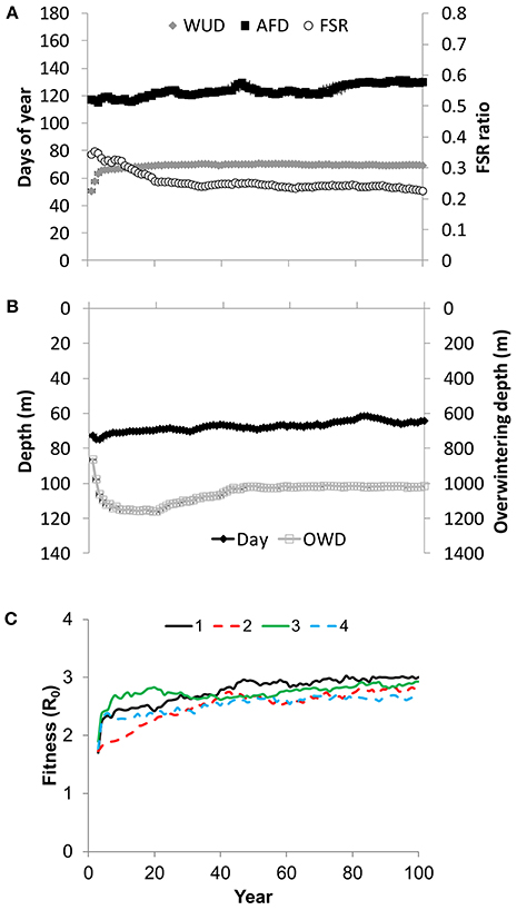
Figure 3. The development over 100 years of the best replicate in simulation 1 in (A) wake up day (WUD), allocation to fat day (AFD) and fat to soma ratio (FSR) traits, (B) the day depth (DD) and overwintering depth (OWD), and (C) fitness (the net reproductive rate, R0) of all four replicates. Values are from end of each year.
Adding inter-annual variability had only a minor effect on the life history trait (Figures 4A,B) compared to the previous simulation. But there was an increase in the day depth to 75 m and thus indicating a more risk averse strategy. There was a pronounced inter-annual variation in the fitness, but only a minor difference between the replicates (Figure 4C). This shows that there is pronounced inter-annual variability in the “productivity” of the forcing data and that this is more important than the increase in fitness due to adaptation process.
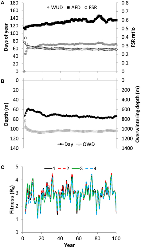
Figure 4. The development over 100 years of the best replicate in simulation 2 in (A) wake up day (WUD), allocation to fat day (AFD) and fat to soma ratio (FSR) traits, (B) the day depth (DD) and overwintering depth (OWD), and (C) fitness (the net reproductive rate, R0) of all four replicates. Values are from end of each year.
In the remaining simulations individuals were initiated over the entire spatial domain and transported with the currents. In simulation 3 individuals were selected randomly from the population at the end of the year before, to contrast the other simulations where the selection probability is proportional to the fitness. The strategies in this case reflected the initiation range in each year and the mean values remained stationary (Figure 5). The fitness was also very low in this simulation and clearly did not reflect viable populations (Figure 5C).
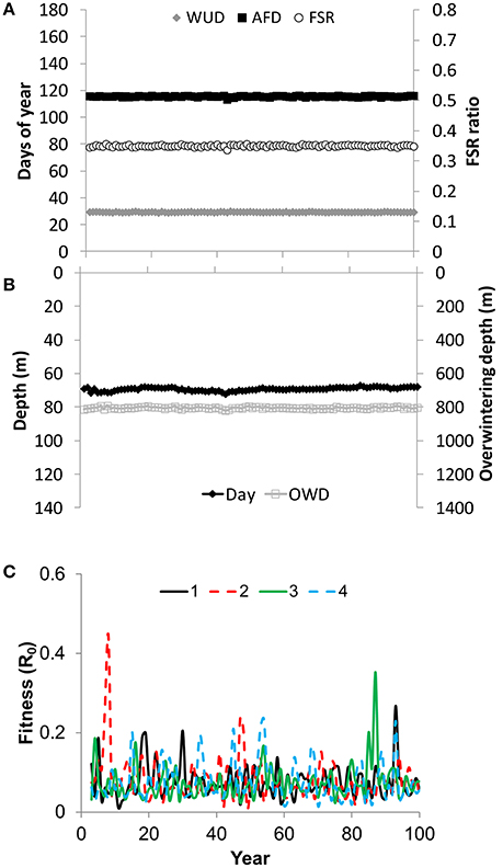
Figure 5. The development over 100 years of the best replicate in simulation 3 in (A) wake up day (WUD), allocation to fat day (AFD) and fat to soma ratio (FSR) traits, (B) the day depth (DD) and overwintering depth (OWD), and (C) fitness (the net reproductive rate, R0) of all four replicates. Values are from end of each year.
In the fourth simulation the forcing in a single year (1983) was repeated over and over. In this case the best strategy had convergent wake up and allocation to fat days at day 100 (Figure 6A). The FSR ratio was slightly increased compared to simulation 1 which did not have the spatial variability. The day depth was at 90 m, which is deeper than in the previous simulations. The four replicates developed slightly differently and the variation between them was more pronounced than in the previous simulations, illustrating the effect of spatial variability (Figures 3, 6). There is also great variation in center of mass (Figure 2) and fitness (Figure 6C) between replicates.
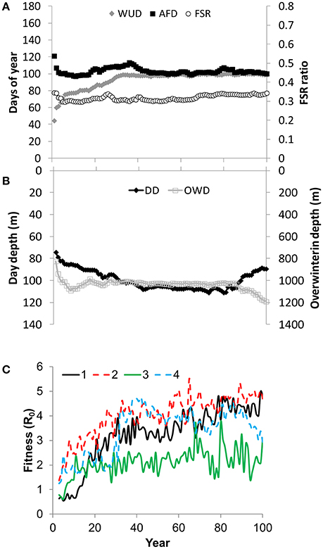
Figure 6. The development over 100 years of the best replicate in simulation 4 in (A) wake up day (WUD), allocation to fat day (AFD) and fat to soma ratio (FSR) traits, (B) the day depth (DD) and overwintering depth (OWD), and (C) fitness (the net reproductive rate, R0) of all four replicates. Values are from end of each year.
In the next simulation the populations were adapted to inter-annual as well as spatial variability in forcing. This simulation (Figure 7) produced a strategy with a slightly delayed ascent compared to the previous simulation and like in the previous simulation (Figure 6), the AFD converged to the WUD value (Figure 7). The day depth was slightly deeper than in the previous simulation. As expected, the fitness was more variable between years, but there was less variation between replicates than in simulation 4 (Figure 6C vs. Figure 7C).
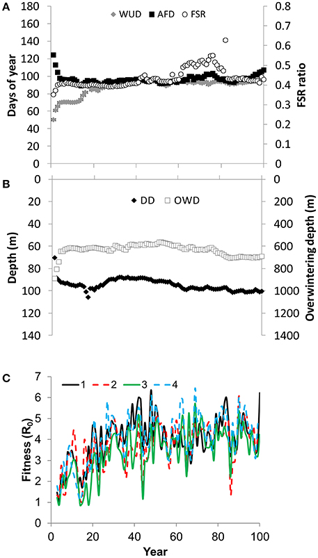
Figure 7. The development over 100 years of the best replicate in simulation 5 in (A) wake up day (WUD), allocation to fat day (AFD) and fat to soma ratio (FSR) traits, (B) the day depth (DD) and overwintering depth (OWD), and (C) fitness (the net reproductive rate, R0) of all four replicates. Values are from end of each year.
Reducing the predator density had a pronounced effect on the time that the simulated copepod spent at the surface. In this simulation the ascent from overwintering (WUD) was on day 120 and the AFD was at day 165, considerably later than for the other simulations. While the day depth was at around 80 m, like many previous simulations, the overwintering depth was at 400 m, and substantially shallower than in all previous simulations (Figure 8B). The peak in the fitness level was increased substantially compared to the previous simulations as expected with the lower predation risk, but there was considerable variation between the replicates (Figure 8C). The highest fitness was associated with the replicate (number 3) that had a center of mass in the central part of the Norwegian Sea, whereas the replicates close to the Norwegian Coast had substantially lower fitness (Figures 2, 8C).
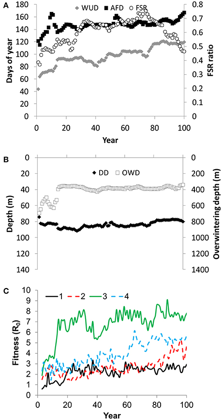
Figure 8. The development over 100 years of the best replicate in simulation 6 in (A) wake up day (WUD), allocation to fat day (AFD) and fat to soma ratio (FSR) traits, (B) the day depth (DD) and overwintering depth (OWD), and (C) fitness (the net reproductive rate, R0) of all four replicates. Values are from end of each year.
When the predator density was increased on the other hand there was not a similar shift in life history (Figure 9) and the WUD and AFD traits were to a large degree similar to simulations 4 and 6 (Figures 6, 8), except that the day depth was deeper than in these simulations. As expected the fitness level was lower in this simulation and about half the level in simulation 6 with decreased predator density. Again there were substantial variation in fitness between the replicates and the lowest fitness was associated with the location close to the Norwegian shore, where one of the replicates had its center of mass (Figures 2, 8C). The other replicates ended up rather closely together to the south of Iceland, but still showed some variation in fitness.
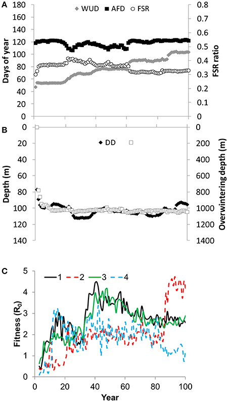
Figure 9. The development over 100 years of the best replicate in simulation 7 in (A) wake up day (WUD), allocation to fat day (AFD) and fat to soma ratio (FSR) traits, (B) the day depth (DD) and overwintering depth (OWD), and (C) fitness (the net reproductive rate, R0) of all four replicates. Values are from end of each year.
The data on seasonal population dynamics were compared for the year 1983, due to the considerable inter-annual variability in the forcing. The seasonal population dynamics varied substantially between the simulations (Figure 10). The highest peak in abundance was found in simulation 6 with reduced predator density. This simulation also had the latest peak, which took place in early September. Simulation 7 with an increased predator density on the other hand, had its peak in abundance 2 months prior, at the end of June. The second highest peak was seen in simulation 4, which was adapted to the year 1983 only. Simulation 5, adapted to inter-annual variability had a lower abundance. The seasonal dynamics of the two simulations without spatial variability (1 and 2) showed an almost identical pattern. The earliest and lowest peak in abundance was in simulation 3 without adaptation as could be expected (Figure 10).
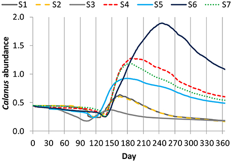
Figure 10. The seasonal development in simulated copepod abundance in the 7 simulations (S1–7) for the year “1983” in the best replicate of each simulation.
One of the objectives of the study was to investigate the importance of the simulated adaptive process on retention and fitness. The results showed that in simulations with adaptation the populations remained viable within the study area of the Norwegian Sea throughout the 100-years, with fitness values much >1. However, in simulation 3 where the individuals were initiated randomly each year without fitness proportional selection of the “best” individuals, the net reproductive rate remained far below 1. This shows that the population was not viable and only upheld due to the procedure of initiating a fixed number of individuals at the start of each year. This illustrates the importance and strength of including adaptation in this type of model.
The simulations with inter-annual variability in forcing (2 and 5) resulted in a pronounced variation in fitness between years. This shows that although the populations adapt to the inter-annual variability, the adaptive process cannot make up for this variability. However, there was not a consistent effect on the trait values. The emergent wake up day was spread out over 2 months in the simulations from day 60 to day 120, with many simulations having an ascent initiated at day 90–100. In most of the simulations the peak in abundance was at day 165–185 (Figure 10). This corresponds well to the timing of the peak in C. finmarchicus abundance seen in the Norwegian Sea (Melle et al., 2004) and to previous model simulations with the NORWECOM.E2E system (Hjøllo et al., 2012). Observations from the Norwegian Sea show that the peak of the spring bloom varies by about 1 month (Rey, 2004), with April 16 (day 106) as the earliest peak day. There was a slight tendency for earlier wake up day in simulation 5 with inter-annual variation compared to simulation 4 without it. Early wake up day makes the copepodites exposed to predation for a longer time span compared to a later wake up. In line with this, simulation 5 had a greater day depth than simulation 4 indicating a more risk averse strategy with inter-annual variability. In the study by Hjøllo et al. (2012) and Samuelsen et al. (2009) it was found that changes in wake up day in spring had several effects on the subsequent population dynamics of the simulated C. finmarchicus population, manifested as changed biomass values/timing and annual production.
In simulations without spatial variability, there were only minor differences between the replicates (Figures 3, 4). However, spatial variability had a strong effect on the fitness variation between the replicates. These simulations produced rather different centers of mass, both between simulations and among replicates (Figure 2). In particular, it was shown that the simulations without inter-annual variability in forcing produced quite different center of mass among replicates, whereas simulation 5 with inter-annual variation in the center of mass was almost identical in the four replicates, and produced populations that remained within the Norwegian Sea. This indicates that there are current structures in some locations in some years that allow local retention of plankton populations. In the model this resulted in local adaptation and widespread centers of mass in the simulations without inter-annual variability. This illustrates how inter-annual variability in current patterns can affect retention in different areas. Plankton are at the “mercy” of this variability and consequently need to be adapted to a range of different environmental situations. This is not new insight and Hjort (1914) formulated his so-called second recruitment hypothesis based on observations of cod larvae out in the Norwegian Sea, far away from their preferred shelf areas in the Barents Sea. Bryant et al. (1998) found that only very restricted parts of the Norwegian Sea around the Faroese Islands and east of Iceland were able to retain simulated copepods over more than 10 years. These areas correspond well to the areas where we found the center of mass of most of the present simulations (Figure 2). Torgersen and Huse (2005) found that there was a low degree of simulated copepod retention in the Norwegian Sea, particularly in the eastern part. After 4 years, only 10% of the simulated copepods remained within the simulated domain. Our model showed that long term persistence is greatly increased in the same area when growth, mortality, reproduction and adaptation of traits are included. To our knowledge there are no other examples of similar long term model simulation with fine resolution in space, time and adaptive individual traits.
Predator density had a pronounced effect both on the population dynamics and behavior. In particular, the individuals adapted under the high predator density evolved a more risk averse strategy with a deeper day depth compared to the simulation with lower predator density. Bollens and Frost (1989) in a classic study found that Calanus pacificus increased the magnitude of their diurnal vertical migration when the density of predator fish was increased. The difference they observed was greater in magnitude than the increase that the present simulations produced which was about 20 m. But the shallowest day depth in simulation 1 was 60 m. The shift from simulation 1 to simulation 6 with increased predator density was 40 m and thus about the same as the shift observed by Bollens and Frost.
Although the traits can be made more dynamic and dependent on local environmental factors, the present strategy vector with six traits works well in adapting the population to the prevailing conditions and shows clearly different adaptive trajectories under different environmental forcing. However, it is easy to modify the day depth calculation so that it for example is related to the local predator density.
Fiksen (2000) with a similar IBM as the present model found the wake up day to be at around day 75 and the allocation to fat day at around day 175. When density dependence was added, the allocation to fat day decreased to around day 150, but nevertheless this span between wake up day and allocation to fat day is quite a bit longer than found in most of the present simulations. We found the span here to be dependent on the predator density and for the lowest predator density (simulation 6) the time span was much greater than in the high predator simulation (simulation 7). This resulted in a delayed peak in copepodite abundance in the low predator simulation compared to the other simulations (Figure 10). This supports the hypothesis proposed by Kaartvedt (2000) that time spent at the surface is minimized to reduce predation risk from pelagic fish that enters the Norwegian Sea to feed in summer. The herring arrives early on the feeding grounds (Dragesund et al., 1997; Holst et al., 2002), but the mackerel arrives later on (Utne et al., 2012b), and avoiding this added predation level is beneficial to the C. finmarchicus.
IBMs are valuable tools for addressing the consequences of different individual traits on for example population dynamics and trophic interactions (Grimm and Railsback, 2005; Neuheimer et al., 2010). Zooplankton can respond to a range of environmental factors including predators, prey, and physical factors such as temperature (Bollens and Frost, 1989; Carlotti et al., 2000; Fiksen, 2000), in the short run by changing their vertical position, and in a longer perspective through life history strategies. The 3D individual based model with emergent life-history and behavior model presented here has been shown to be useful for investigating how different trait formulations affect the population dynamics and behavior of plankton. There are a range of different hypotheses related to diapauses initiation and termination in C. finmarchicus (Hirche, 1996a; Heath, 1999; Fiksen, 2000; Heath et al., 2000), and the present model system is ideal for investigating the consequences of such hypotheses for the spatial and population dynamics of plankton. We based our 3D model on the traits used by Fiksen (2000), who studied evolutionary robust strategies in a 1D model of C. finmarchicus. This approach has previously been used to study migrations (Huse and Giske, 1998; Huse, 2001; Strand et al., 2002) and life history traits (Huse and Ellingsen, 2008) in fish.
To model the demography of C. finmarchicus in the north-east Atlantic, Speirs et al. (2006) used a full C. finmarchicus life cycle model forced by phytoplankton through satellite observations and modeled weekly updated physical transport of individuals from one cell to another in two distinct layers (20 and 600 m). They found that transport was generally not important to demography, but that there was a strong connectivity of C. finmarchicus within the entire distribution area of the species. Their approach is computationally efficient and allows statistical parameter fitting, but lacks a fully resolved flow field and the feedback between the different tropic layers. The NORWECOM.E2E model considers feedbacks between the different trophic levels and driven by realistic physical forcing have been developed, and also extended to include pelagic fish. The present simulations did, however, not include feedback to allow long term simulations for studying retention and evolve traits.
The simulations relied on a rather low initial population size. This makes the run time fast and allows multiple simulations and replicates. However, there are potential downsides to this related to only finding local minima in the fitness landscape as well as covering only restricted geographic locations within the large simulation area. Hjøllo et al. (2012) found that the aggregated variables such as production was sensitive to the number of super individuals simulated. They found a 10% lower production for a simulation with 23,000 individuals compared to the reference simulation with 200,000 individuals, but simulations with 47,000 and 120,000 super individuals have about the same cumulative production as in the reference run.
Several approaches have been taken to simulate the spatial and population dynamics of copepods both using 1D Individual Based Models (IBMs) (Carlotti and Nival, 1992; Carlotti et al., 1993; Carlotti and Radach, 1996; Carlotti and Wolf, 1998), 3D IBMs (Miller et al., 1998; Pedersen et al., 2001; Tittensor et al., 2003), and 3D Eulerian (Speirs et al., 2005, 2006) models (reviewed by Gentleman, 2002). While IBMs have individuals as the unit for calculation, Eularian models have spatial locations as the basic unit and considers the dynamics in locations as a function of local population dynamics, imports, and loss (Carlotti et al., 2000) The different approaches have their pros and cons and the Eularian models are in general numerically more efficient than IBMs, which on the other hand allow a more detailed biological description of individuals.
The resampling scheme introduced here with a fixed initial abundance at the start of each year, provides a simple approach to keep the number of super individuals simulated under control without constraining the ecological or evolutionary processes too much. This allows for rather long term simulations, over 100 years with a simulation time of a few hours on a laptop. Feedback on the phytoplankton is not included presently, but since this is known to be important in many areas, fully coupled model systems are developed. The models based on IBMs have much longer simulation time as more super individuals are needed to cover the geographical area and provide realistic forage feedback. An application of the present model is therefore to produce robust strategy vectors for use in fully coupled end to end models such as NORWECOM.E2E (Hjøllo et al., 2012; Utne et al., 2012a). Although the present offline version is valuable for providing a starting point for simulations, it is likely that the selection pressure will change slightly as a response to the density dependent food availability in the fully coupled model. This may create a “drift” in the strategy vectors that requires either to use some further adaptation or to use fixed strategy vectors for the population.
GH had the idea for the paper and contributed to coding and writing of paper. MS and SH contributed to coding and writing. WB made contributions on the physics data used to force the biological model and contributed description of text. WM and ES contributed to writing.
The authors declare that the research was conducted in the absence of any commercial or financial relationships that could be construed as a potential conflict of interest.
The work was supported by the Research Council of Norway, the European Commission through the projects MEECE (Grant number 212085) and EUROBASIN (ENV.2010.2.2.1-1) (Contract number 264993), and the Institute of Marine Research.
Aksnes, D. L., and Blindheim, J. (1996). Circulation patterns in the North Atlantic and possible impact on population dynamics of Calanus finmarchicus. Ophelia 44, 7–28. doi: 10.1080/00785326.1995.10429836
Aksnes, D. L., and Giske, J. (1993). A theoretical-model of aquatic visual feeding. Ecol. Modell. 67, 233–250. doi: 10.1016/0304-3800(93)90007-F
Aksnes, D. L., Ulvestad, K. B., Baliño, B. M., Berntsen, J., Egge, J. K., and Svendsen, E. (1995). Ecological modelling in coastal waters: towards predictive physical-chemical-biological simulation models. Ophelia 41, 5–36. doi: 10.1080/00785236.1995.10422035
Aksnes, D. L., and Utne, A. C. W. (1997). A revised model of visual range in fish. Sarsia 82, 137–147. doi: 10.1080/00364827.1997.10413647
Bollens, S. M., and Frost, B. W. (1989). Zooplanktivorous fish and variable diel vertical migration in the marine planktonic copepod Calanus pacificus. Limnol. Oceanogr. 34, 1072–1083. doi: 10.4319/lo.1989.34.6.1072
Brown, J. S., Laundré, J. W., and Gurung, M. (1999). The ecology of fear: optimal foraging, game theory, and trophic interactions. J. Mammal. 80, 385–399. doi: 10.2307/1383287
Bryant, A. D., Hainbucher, D., and Heath, M. (1998). Basin-scale advection and population persistence of Calanus finmarchicus. Fish. Oceanogr. 7, 235–244. doi: 10.1046/j.1365-2419.1998.00074.x
Campbell, R. G., Wagner, M. M., Teengarden, G. J., Boudreau, C. A., and Durbin, E. G. (2001). Growth and development rates of the copepod Calanus finmarchicus reared in the laboratory. Mar. Ecol. Prog. Ser. 221, 161–183. doi: 10.3354/meps221161
Carlotti, F., Giske, J., and Werner, F. (2000). “Modeling zooplankton dynamics,” in ICES Zooplankton Methodolgy Manual, eds R. Harris, P. Wiebe, J. Lenz, H. R. Skjoldal, and M. Huntley (London: Academic Press), 571–667.
Carlotti, F., Krause, M., and Radach, G. (1993). Growth and development of Calanus finmarchicus related to the influence of temperature: experimental results and conceptual model. Limnol. Oceanogr. 38, 1125–1134. doi: 10.4319/lo.1993.38.6.1125
Carlotti, F., and Nival, P. (1992). Model of copepod growth and development: moulting and mortality in relation to physiological processes during an individual moult cycle. Mar. Ecol. Prog. Ser. 84, 219–233. doi: 10.3354/meps084219
Carlotti, F., and Radach, G. (1996). Seasonal dynamics of phytoplankton and Calanus finmarchicus in the North Sea as revealed by a coupled one-dimensional model. Limnol. Oceanogr. 41, 522–539. doi: 10.4319/lo.1996.41.3.0522
Carlotti, F., and Wolf, K. U. (1998). A Lagrangian ensemble model of Calanus finmarchicus coupled with a 1-D ecosystem model. Fish. Oceanogr. 7, 191–204. doi: 10.1046/j.1365-2419.1998.00085.x
Chambers, C. R. (1993). Phenotypic variability in fish populations and its representation in individual-based models. Trans. Am. Fish. Soc. 122, 404–414. doi: 10.1577/1548-8659(1993)122<0404:PVIFPA>2.3.CO;2
Creel, S., and Christianson, D. (2008). Relationships between direct predation and risk effects. Trends Ecol. Evol. 23, 194–201. doi: 10.1016/j.tree.2007.12.004
Dragesund, O., Johannessen, A., and Ulltang, Ø. (1997). Variation in migration and abundance of Norwegian spring spawning herring (Clupea harengus L.). Sarsia 82, 97–105. doi: 10.1080/00364827.1997.10413643
Eiane, K., Aksnes, D. L., and Ohman, M. D. (1998). Advection and zooplankton fitness. Sarsia 83, 87–93. doi: 10.1080/00364827.1998.10413674
Fiksen, O. (2000). The adaptive timing of diapause – a search for evolutionarily robust strategies in Calanus finmarchicus. ICES J. Mar. Sci. 57, 1825–1833. doi: 10.1006/jmsc.2000.0976
Gentleman, W. (2002). A chronology of plankton dynamics in silico: how computer models have been used to study marine ecosystems. Hydrobiologia 480, 69–85. doi: 10.1023/A:1021289119442
Giske, J., Aksnes, D. L., and Førland, B. (1993). Variable generation time and Darwinian fitness measures. Evol. Ecol. 7, 233–239. doi: 10.1007/BF01237741
Grimm, V., Berger, U., Bastiansen, F., Eliassen, S., Ginot, V., Giske, J., et al. (2006). A standard protocol for describing individual-based and agent-based models. Ecol. Modell. 198, 115–126. doi: 10.1016/j.ecolmodel.2006.04.023
Grimm, V., and Railsback, S. F. (2005). Individual-Based Modeling and Ecology. Princeton: Princeton University Press.
Haidvogel, D. B., Arango, H. G., Hedstrom, K., Beckmann, A., Malanotte-Rizzoli, P., and Shchepetkin, A. F. (2000). Model evaluation experiments in the North Atlantic Basin: simulations in nonlinear terrain-following coordinates. Dyn. Atmos. Oceans 32, 239–281. doi: 10.1016/S0377-0265(00)00049-X
Heath, M. R. (1999). The ascent migration of Calanus finmarchicus from overwintering depths in the Faroe-Shetland Channel. Fish. Oceanogr. 8, 84–99. doi: 10.1046/j.1365-2419.1999.00013.x
Heath, M. R., Fraser, J. G., Gislason, A., Hay, S. J., Jonasdottir, S. H., and Richardson, K. (2000). Winter distribution of Calanus finmarchicus in the Northeast Atlantic. ICES J. Mar. Sci. 57, 1628–1635. doi: 10.1006/jmsc.2000.0978
Hirche, H. J. (1996a). Diapause in the marine copepod, Calanus finmarchicus- a review. Ophelia 44, 129–143. doi: 10.1080/00785326.1995.10429843
Hirche, H. J. (1996b). The reproductive biology of the marine copepod, Calanus finmarchicus- a review. Ophelia 44, 111–128. doi: 10.1080/00785326.1995.10429842
Hjøllo, S. S., Huse, G., Skogen, M. D., and Melle, W. (2012). Modelling secondary production in the Norwegian Sea with a fully coupled physical/primary production/individual-based Calanus finmarchicus model system. Mar. Biol. Res. 8, 508–526. doi: 10.1080/17451000.2011.642805
Hjort, J. (1914). Fluctuations in the great fisheries of northern Europe reviewed in the light of biological research. Rapp Proc Verb Réun Cons. Int. l'Explor Mer 20, 1–28
Holst, J. C., Dragesund, O., Hamre, J., Misund, O. A., and Østvedt, O. J. (2002). Fifty years of herring migrations in the Norwegian Sea. ICES Mar. Sci. Symposia 215, 352–360.
Huse, G. (1998). Life History Strategies and Spatial Dynamics of the Barents Sea Capelin (Mallotus villosus). Bergen: University of Bergen.
Huse, G. (2001). Modelling habitat choice in fish using adapted random walk. Sarsia 86, 477–483. doi: 10.1080/00364827.2001.10420487
Huse, G. (2005). Artificial evolution of Calanus' life history strategies under different predation levels. Globec International Newsletter, Book 11.
Huse, G., and Ellingsen, I. H. (2008). Capelin migrations and climate change - a modelling analysis. Clim. Change 87, 177–191. doi: 10.1007/s10584-007-9347-z
Huse, G., and Giske, J. (1998). Ecology in Mare Pentium: an individual-based spatio-temporal model for fish with adapted behaviour. Fish. Res. 37, 163–178. doi: 10.1016/S0165-7836(98)00134-9
Huse, G., Giske, J., and Salvanes, A. G. V. (2002). “Individual-based models,” in Handbook of Fish and Fisheries, Book 2, eds P. J. B. Hart and J. Reynolds (Oxford: Blackwell Science), 228–248.
Huse, G., Strand, E., and Giske, J. (1999). Implementing behaviour in individual-based models using neural networks and genetic algorithms. Evol. Ecol. 13, 469–483. doi: 10.1023/A:1006746727151
Kaartvedt, S. (2000). Life history of Calanus finmarchicus in the Norwegian Sea in relation to planktivorous fish. ICES J. Mar. Sci. 57, 1819–1824. doi: 10.1006/jmsc.2000.0964
Marshall, S. M., and Orr, A. P. (1955). The Biology of a Marine Copepod. Edinburgh; London: Oliver and Boyd.
Melle, W., Ellertsen, B., and Skjoldal, H. R. (2004). “Zooplankton: the link to higher trophic levels,” in The Norwegian Sea Ecosystem, ed H. R. Skjoldal (Trondheim: Tapir Academic Press), 137–202.
Miller, C. B., Lynch, D. R., Carlotti, F., Gentleman, W., and Lewis, C. V. W. (1998). Coupling of an individual-based population dynamic model of Calanus finmarchicus to a circulation model for the Georges Bank region. Fish. Oceanogr. 7, 219–234. doi: 10.1046/j.1365-2419.1998.00072.x
Mitchell, M., and Forrest, S. (1995). “Genetic algorithms and artificial life,” in Artificial Life: An overview, ed C. G. Langton (Cambridge, MA: The MIT Press).
Neuheimer, A. B., Gentleman, W. C., Pepin, P., and Head, E. J. H. (2010). How to build and use individual-based models (IBMs) as hypothesis testing tools. J. Mar. Syst. 81, 122–133. doi: 10.1016/j.jmarsys.2009.12.009
Ohman, M. D., Eiane, K., Durbin, E. G., Runge, J. A., and Hirche, H. J. (2004). A comparative study of Calanus finmarchicus mortality patterns at five localities in the North Atlantic. ICES J. Mar. Sci. 61, 687–697. doi: 10.1016/j.icesjms.2004.03.016
Pedersen, O. P., Tande, K. S., and Slagstad, D. (2001). A model study of demography and spatial distribution of Calanus finmarchicus at the Norwegian coast. Deep Sea Res. II Top. Stud. Oceanogr. 48, 567–587. doi: 10.1016/S0967-0645(00)00127-2
Rey, F. (2004). “Phytoplankton: the grass of the sea,” in The Norwegia Sea Ecosystem, ed H. R. Skjoldal (Trondheim: Tapir Academic Press), 97–136.
Samuelsen, A., Huse, G., and Hansen, C. (2009). Shelf recruitment of Calanus finmarchicus off the west coast of Norway: role of physical processes and timing of diapause termination. Mar. Ecol. Prog. Ser. 386, 163–180. doi: 10.3354/meps08060
Scheffer, M., Baveco, J. M., DeAngelis, D. L., Rose, K. A., and van Nes, E. H. (1995). Super-individuals a simple solution for modelling large populations on an individual basis. Ecol. Modell. 80, 161–170. doi: 10.1016/0304-3800(94)00055-M
Skartveit, A., and Olseth, J. A. (1988). Varighetstabeller for Timevis Belysning Mot 5 Flater på 16 Norske Stasjoner. Bergen, University of Bergen.
Skjoldal, H. R., Dalpadado, P., and Dommasnes, A. (2004). “Food webs and trophic interactions,” in The Norwegian Sea Ecosystem, ed H. R. Skjoldal (Bergen: Tapir Academic Press), 447–506.
Skogen, M. D., Budgell, W. P., and Rey, F. (2007). Interannual variability in Nordic seas primary production. ICES J. Mar. Sci. 64, 889–898. doi: 10.1093/icesjms/fsm063
Søiland, H., and Huse, G. (2012). Using RAFOS floats to simulate overwinter transport of Calanus finmarchicus in the Norwegian Sea. Mar. Biol. Res. 8, 502–507. doi: 10.1080/17451000.2011.639780
Speirs, D. C., Gurney, W. S. C., Heath, M. R., Horbelt, W., Wood, S. N., and de Cuevas, B. A. (2006). Ocean-scale modelling of the distribution, abundance, and seasonal dynamics of the copepod Calanus finmarchicus. Mar. Ecol. Prog. Ser. 313, 173–192. doi: 10.3354/meps313173
Speirs, D. C., Gurney, W. S. C., Heath, M. R., and Wood, S. N. (2005). Modelling the basin-scale demography of Calanus finmarchicus in the north-east Atlantic. Fish. Oceanogr. 14, 333–358. doi: 10.1111/j.1365-2419.2005.00339.x
Strand, E., Huse, G., and Giske, J. (2002). Artificial evolution of life history and behavior. Am. Nat. 159, 624–644. doi: 10.1086/339997
Tittensor, D. P., Deyoung, B., and Tang, C. L. (2003). Modelling the distribution, sustainability and diapause emergence timing of the copepod Calanus finmarchicus in the Labrador Sea. Fish. Oceanogr. 12, 299–316. doi: 10.1046/j.1365-2419.2003.00266.x
Torgersen, T., and Huse, G. (2005). Variability in retention of Calanus finmarchicus in the Nordic Seas. ICES J. Mar. Sci. 62, 1301–1309. doi: 10.1016/j.icesjms.2005.05.016
Utne, K. R., Hjøllo, S. S., Huse, G., and Skogen, M. (2012a). Estimating consumption of Calanus finmarchicus by planktivorous fish in the Norwegian Sea estimated fromusing a fully coupled 3D model system. Mar. Biol. Res. 8, 527–547. doi: 10.1080/17451000.2011.642804
Utne, K. R., and Huse, G. (2012). Estimating the horizontal and temporal overlap of pelagic fish distribution in the Norwegian Sea using individual-based modelling. Mar. Biol. Res. 8, 548–567. doi: 10.1080/17451000.2011.639781
Keywords: individual based models, Calanus finmarchicus, emergent properties, ecology, Norwegian sea
Citation: Huse G, Melle W, Skogen MD, Hjøllo SS, Svendsen E and Budgell WP (2018) Modeling Emergent Life Histories of Copepods. Front. Ecol. Evol. 6:23. doi: 10.3389/fevo.2018.00023
Received: 01 March 2016; Accepted: 27 February 2018;
Published: 21 March 2018.
Edited by:
Michael Arthur St. John, National Institute of Aquatic Resources, Technical University of Denmark, DenmarkReviewed by:
Mario Barletta, Departamento de Oceanografia da Universidade Federal de Pernambuco (UFPE), BrazilCopyright © 2018 Huse, Melle, Skogen, Hjøllo, Svendsen and Budgell. This is an open-access article distributed under the terms of the Creative Commons Attribution License (CC BY). The use, distribution or reproduction in other forums is permitted, provided the original author(s) and the copyright owner are credited and that the original publication in this journal is cited, in accordance with accepted academic practice. No use, distribution or reproduction is permitted which does not comply with these terms.
*Correspondence: Geir Huse, Z2Vpci5odXNlQGhpLm5v
Disclaimer: All claims expressed in this article are solely those of the authors and do not necessarily represent those of their affiliated organizations, or those of the publisher, the editors and the reviewers. Any product that may be evaluated in this article or claim that may be made by its manufacturer is not guaranteed or endorsed by the publisher.
Research integrity at Frontiers

Learn more about the work of our research integrity team to safeguard the quality of each article we publish.