Implications of groundwater level changes before near field earthquakes and its influencing factors - several earthquakes in the vicinity of the Longmenshan-Anninghe fault as an example

Characteristics of groundwater level changes may be correlated with subsequent earthquake events. However, the relationship and its determining factors remain unclear. This study examines eight wells situated near the Longmenshan-Anninghe fault zone, which exhibit significant disparities in changes of groundwater level. We quantified these changes by Molchan diagram and investigated factors that may affect it using correlation assessments. The results indicate groundwater levels changes that are more responsive to static stresses and tidal forces also have a high correlation with subsequent earthquake events. Specific leakage, a hydraulic parameter, also effects the correlation between groundwater levels and subsequent earthquakes. Spatial distribution of epicenters may also contribute to differences in this correlation, while aquifer confinement appears to have minimal effect. We used a random forest regression to calculate the comprehensive contribution of these factors to the correlation between groundwater levels and subsequent earthquakes. Notably, epicenter locations showcase the utmost sensitivity to this correlation. These findings can help us understand the complex mechanisms of water level changes before earthquakes and provide insights into the optimal locations for monitoring boreholes.

1 Introduction

As an active element capable of responding positively to crustal stresses, hydrological changes in groundwater due to seismic effects have been widely documented (Barberio et al., 2020; Del Gaudio et al., 2024; Granin et al., 2018; Hattori and Han, 2018; Pulinets et al., 2018; Zhang et al., 2023), with pre-earthquake anomalies in groundwater levels being a consistent observation. For instance, the 1975 Haicheng earthquake in China was successfully predicted due to anomalies detected at numerous hydrological monitoring sites (Wang et al., 2006). Similarly, prior to the 1985 California Ms6.1 earthquake, two wells in close proximity exhibited a remarkable 3-cm rise in groundwater level (Roeloffs et al., 1997). In the case of the 1999 Ms7.7 Taiwan Chi-Chi earthquake, anomalous downward changes in water level were detected in several monitoring wells located on a nearby alluvial fan within a 200-day period (Chen et al., 2015). Through retrospective analysis, it was detected that groundwater level changes before multiple earthquakes in the Kamchatka Peninsula were highly correlated with subsequent earthquakes (Kopylova and Boldina, 2020). Additionally, Prior to the 2008 Wenchuan Ms8.0 earthquake in China, an increase in high-frequency anomalies was observed in the water level of wells near the Longmenshan Fracture (Sun et al., 2016). Yan et al. (2018) found a significant increase in anomalies at three times the rupture scale in the 5 months preceding the Wenchuan Ms8.0 earthquake. These studies underscore the potential of groundwater level anomalies as the means for earthquake prediction.

While numerous pre-earthquake water level anomalies have been observed in monitoring wells, the earthquake prediction utilizing water level changes remains largely challenging. The primary obstacle is the complex formation mechanism of groundwater level precursors, which is not yet fully understood. Furthermore, a comprehensive quantitative framework to account for various factors influencing groundwater levels during seismic events is often lacking. The direct establishment of a one-to-one connection between groundwater level changes and the occurrence of earthquakes is elusive, thereby placing limitations on the reliability of using groundwater level changes as sole indicator of earthquake occurrence.

Since earthquake precursors are difficult to capture, and it is difficult to find a one-to-one correspondence between tectonic stress and groundwater level precursors. Mathematical-statistical methods, such as the Molchan diagram method (Molchan, 1990), have become increasingly accepted in the probabilistic prediction of earthquakes. These methods analyze the statistical relationship between seismic event triggers and the corresponding changes in observed groundwater levels. Their purpose is identifying mathematical relationships that can approximate the underlying connection between these two phenomena. Molchan (1990) introduced the use of loss functions to predict arbitrary points, while Zechar and Jordan (2008) enhanced Molchan’s method, enabling comprehensive probabilistic prediction of three elements of earthquakes. Sun et al. (2017) employed the Molchan diagram method to analyze hydrological data, thereby quantitatively assessing the ability reflecting earthquake of groundwater level through the utilization of water temperature anomalies as a discriminating factor. Lai et al. (2021) employed the Molchan diagram method to assess the short- and medium-term predictive capabilities of subsurface fluid dynamics by incorporating the correlation between groundwater level and temperature data. These studies highlight that the Molchan method can effectively filter out groundwater level changes from a large amount of data and can indicate the correlation between groundwater level changes and subsequent earthquakes.

At present, there is still a lack of success in accurately predicting earthquakes, but models such as statistics and machine learning can help us mine potential information from a large amount of observational data and past events to aid in understanding the complex process of groundwater level changes. Therefore, we select the Molchan method to quantify the characteristics of groundwater level changes before earthquakes, and further determines the factors that control groundwater level changes through wavelet analysis, leaky aquifer model and random forest regression.

This study seeks to quantitatively evaluate potential factors that exert influence on characteristics of groundwater level changes before earthquakes in eight wells located in Longmenshan-Anninghe faults zone. Based on observed groundwater level data, we focus on the correlation between groundwater level changes characteristics and aquifer confinement, hydraulic parameters, earthquake epicenter orientation, response to tidal effect and seismic static stresses. Additionally, sensitivity analysis was conducted to identify the dominant factors that influence groundwater level changes characteristics. This approach can systematically reveal the reasons behind the variability in forecasting accuracy observed across different monitoring wells. Limited by the lack of theoretical research, this paper initially reveals the drivers of groundwater level changes before earthquakes by using a combination of Molchan Diagram, Wavelet Coherence Analysis, and Random Forest Regression. Additionally, it will offer guidance for future monitoring of seismic fluid activities.

2 Background to the study

2.1 Backgrounds

The Longmenshan Fault, positioned critically between the Tibetan Plateau and the Sichuan Basin, extends impressively over a length exceeding 500 km and spans approximately 70 km in width, featuring a northeast-southwest strike (Figure 1). The fault zone is subject to continuous compression from the Tibetan Plateau in the northwest, resulting in highly active geological activity (Zhang, 2008). Throughout the Late Quaternary period, the fault zone’s activity has exhibited a gradual intensification from north to south. The fault zone is developed within a metamorphic heterogeneous rock body, characterized by high rupture intensity, thereby facilitating energy accumulation and predisposing the area to the occurrence of powerful earthquakes. Since the 1960s, “Y”-shaped fault zone (F1, F2, and F3 in Figure 1) has experienced a total of seven earthquakes with magnitudes of 7.0 or greater in Sichuan Province, establishing it as the most active region for strong earthquakes in western mainland China (Bai et al., 2019). The 2008 Wenchuan Ms8.0 earthquake has generated large ruptures of up to 300 km in length beneath the surface, occurring within an exceptionally brief time frame. The central rupture zone has been observed to span approximately 240 km (Zhang et al., 2008).

Figure 1

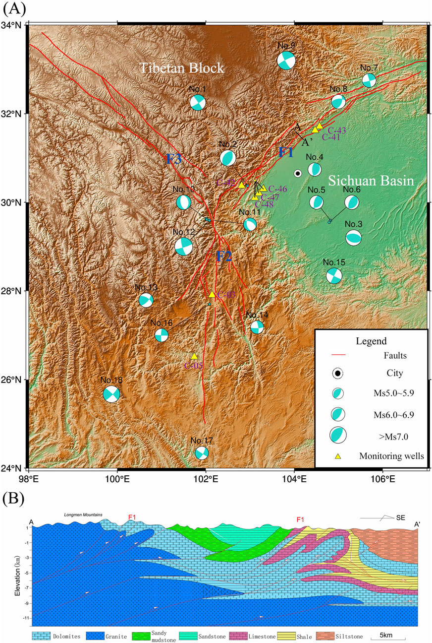
Figure 1. Locations of 8 wells and the 18 earthquakes. (A) The “beach balls” show the focal mechanism for earthquakes. Red lines show the faults, F1 is the Longmenshan Fault, F2 is the Anninghe Fault, and F3 is the Xianshuihe Fault. The yellow triangles indicate the monitoring wells. (B) The geological sections across F1 are shown at A-A’.

Emerging from the southernmost segment of the Longmenshan fault zone, the Anninghe fault constitutes an additional region prone to frequent seismic activity. This fault, extending in a north-south direction, is predominantly characterized by sinistral strike-slip faults. It spans approximately 170 km in length and exhibits a complex hierarchical structure (Yi et al., 2004). Occupying a pivotal role, the Anninghe fault has been the site of a series of earthquakes (He and Ikeda, 2007).

2.2 Selections of monitoring wells and earthquakes

Following the statistical relationship between magnitude and distance as detailed in the “China Seismic Code,” the study selected earthquakes at a certain distance from the monitoring wells, near the Longmenshan-Anninghe Faults (98–107°N, 24–34°E). Specifically, earthquakes of magnitude Ms5.0-6.0 were chosen within a 250 km seismic distance from the wells, earthquakes of magnitude Ms6.0-7.0 within 300 km and those of Ms7.0 or higher within 500 km (Table 1). This provides reasonable assurance that all monitoring wells will be within the range of seismic static strain (Shi et al., 2013). The earthquake time frame selection criteria are based on recent earthquake occurrences (2017–2023) and the inclusion of a wide range of magnitudes, particularly focusing on earthquakes above magnitude 5 and 6 to ensure methodological compatibility. Moreover, the groundwater level time series is selected within the same 2017-2023 timeframe to correspond with the seismic events under investigation. The surface wave magnitude (Ms) was chosen as the magnitude type for this paper, which was determined by measuring Rayleigh wave amplitudes at periods of approximately 20 s. Unlike Local magnitude (ML), which is calibrated for regional distances (<600 km) and specific to local crustal structures. Moment magnitude (Mw), based on the seismic moment tensor solution, provides the most complete physical description of earthquake size by considering fault parameters. However, Ms remains the standard scale in China, particularly effective for shallow earthquakes (depth <70 km) and historical catalog comparisons. A total of eight groundwater monitoring wells, depicted in Figure 1, were chosen for this study to ensure a better correspondence with the earthquakes. Some wellbore and stratigraphical are shown in Figure 2. Monitoring wells were deployed by the China Earthquake Administration (CEA) and were equipped with LN-3 and ZKGD3000-N groundwater level detectors, recording at a frequency of one measurement per minute, 1 mm resolution and 0.2% F.S. The original groundwater level curves and the difference curves are illustrated in Figure 3. Difference curves are calculated using first-order differences, which helps in highlighting changes in the rate of change of ground water level. The key information regarding the monitoring wells and their related features are outlined in Table 2.

Table 1

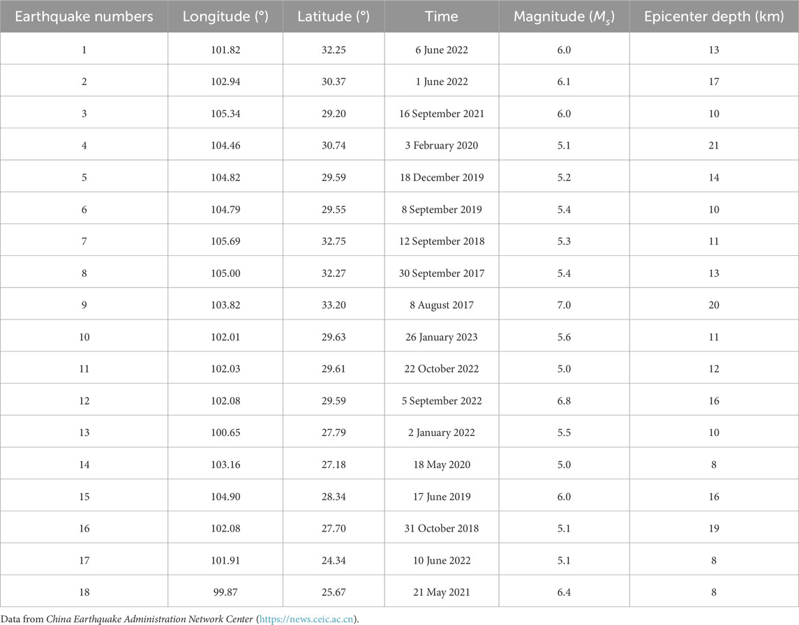
Table 1. Basic information of 18 earthquakes.

Figure 2

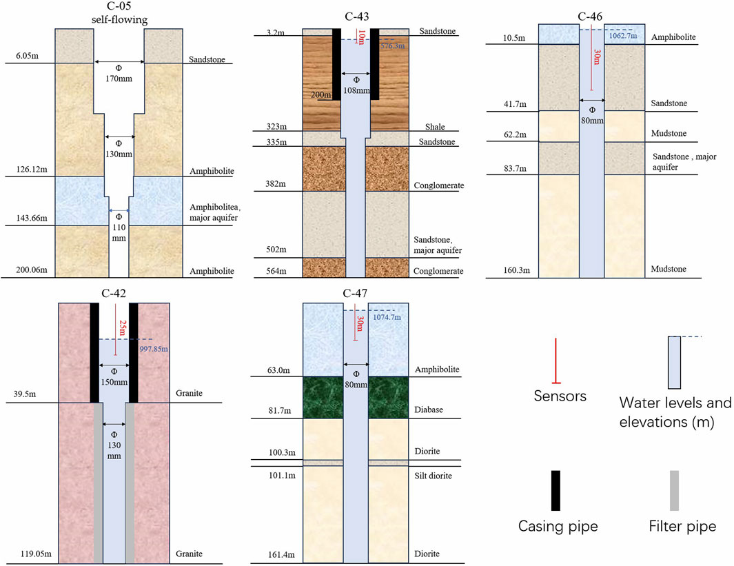
Figure 2. Partial wellbores structure and their lithology. The water level is converted from the water pressure measured by the sensor; the depth of the monitoring probe inside the wells refers to the distance from the sensor to the surface.

Figure 3

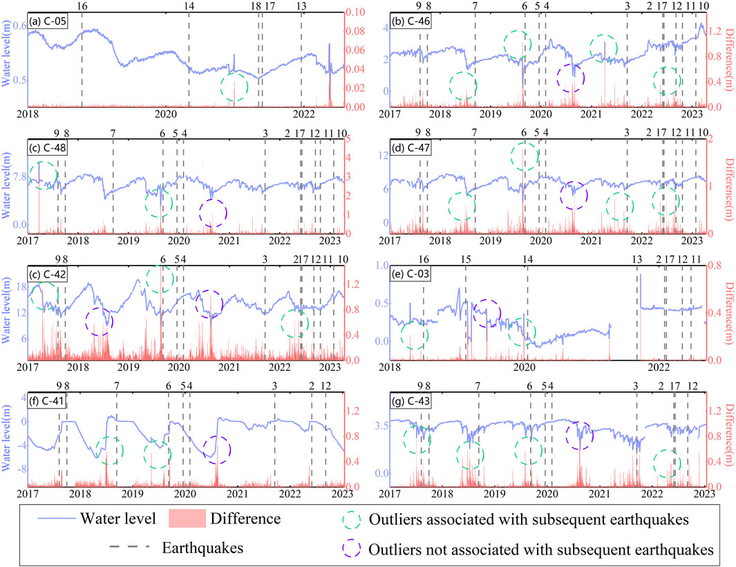
Figure 3. Daily water level and differential values of the 8 wells. The blue lines indicate the Water level and the red curve show the differential values. The water level here is the distance between the surface of the water in the well and the surface of the ground, a positive value means that the water level is below the surface and a negative value means that it is above the surface. The black dashed line shows the seismic events that occurred during the study time in Table 1. The differentials represented by the green and purple circles show elevated values that markedly exceed those of their surroundings, which is a suspected anomaly. The key distinction is that the anomalies within the green circles are associated possibly with subsequent earthquakes, whereas the purple circle anomalies are not.

Table 2

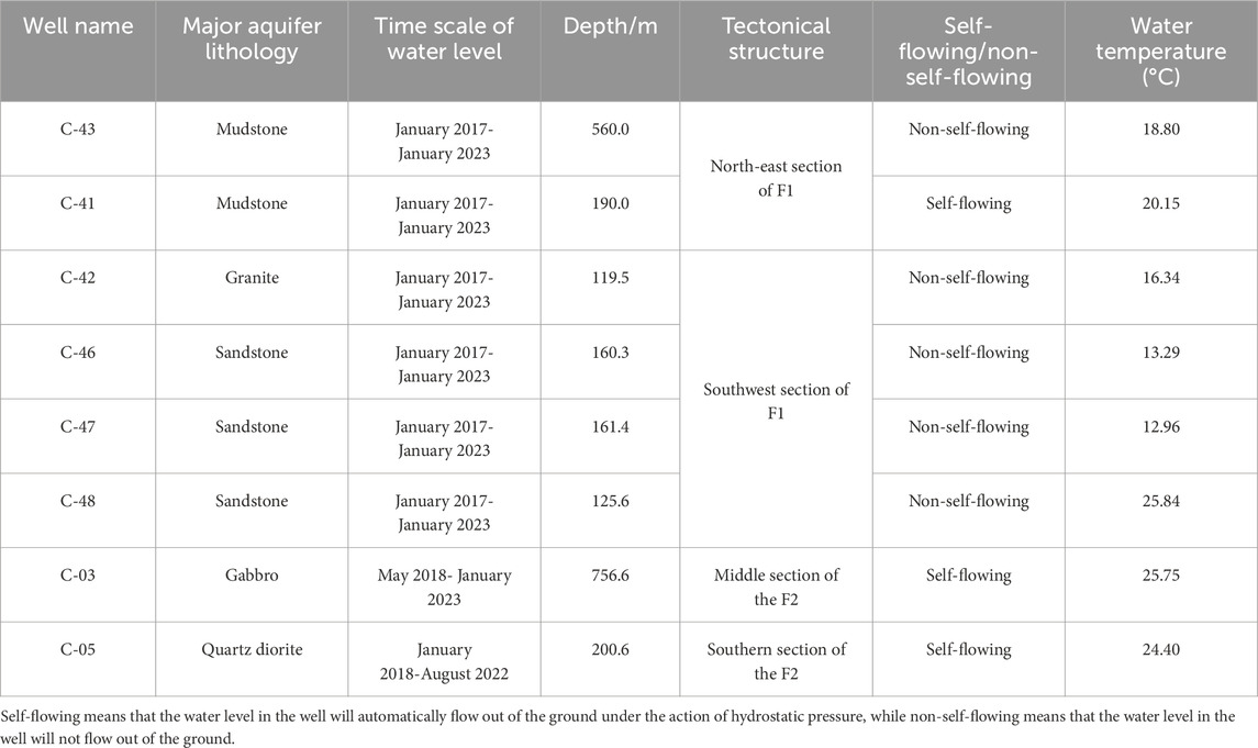
Table 2. Basic Information of the 8 wells.

3 Methods

3.1 Molchan diagram test

The Molchan diagram method offers a quantitative approach to assess the correspondence between groundwater level changes and subsequent events (Molchan, 1990; Zechar and Jordan, 2008). It involves establishing various differential thresholds to calculate the Abnormal time period occupancy rate τ and the Miss rate v can be calculated. These values are then plotted as τ-v step lines within the Molchan diagram, also known as the Molchan test line. The position of the step lines determines the strength of the correlation between groundwater level changes and subsequent earthquakes (Molchan, 1990; Zechar and Jordan, 2008). Molchan diagram requires the assessment of probability Gain and significance, and the equations involved and the significance of the parameters are as follows (Zechar and Jordan, 2008):

$Gain=\frac{h}{\tau }=\frac{1-v}{\tau }(1)$

$B\left(h|N,\tau \right)=C_h^N{\tau }^h{\left(1-\tau \right)}^{N-h}(2)$

where h is the number of hits: the number of earthquakes that successfully landed in the alarm region; v is the miss rate: The ratio of earthquakes not falling within the alarm region to the total number of earthquakes; τ is the abnormal time period occupancy rate: the ratio of the anomalous time horizon of the groundwater level to the total; B is the cumulative binomial distribution, which is used to test for statistical significance; and N is the number of random hits. Gain is determined by the combination of v and τ, and the length of the time period does not affect the results. The closer the Molchan test line is to the line of greater probability gain, the better its overall prediction. For convenience, we define the normalized area to the right of the Molchan test line as the pre-response index (PRI), that is, the potential of groundwater level to reflect subsequent earthquakes. The PRI range is 0–1, and the closer it is to 1, the stronger the correlation between groundwater level changes and subsequent events. The PRI value changes with the position of the Molchan test line (Sun et al., 2017).

In this study, a criterion is established to differentiate between high and low PRI. This criterion is based on setting a threshold value that reflects the absolute magnitude of differential values. Differences that exceed the threshold value are identified as anomalous. The alarm area will be set within a certain period of time after anomalous. An earthquake is deemed to have been successfully hit if it occurs both within the alarm area. Conversely, a hit is regarded as unsuccessful if the earthquake happens outside of the alarm area. To facilitate understanding, let’s consider the example of well C-48 for a 94-day period from 1 July 2018, to 1 October 2018 (Figure 4). We will set the alarm area as 10 days.

a) When the threshold line is set to 0.5, only the value of July 3 is determined to be anomalous. At this time, according to Equations 1, 2, τ = (1 + 10)/94 = 0.12. The 7th earthquake does not fall within the alarm area, thereby v = 1/1 = 1.

b) When the threshold line is set to 0.25, there are 7 days of values exceeding the threshold. The last anomaly, which occurs in September 16 after the 10-day alarm area, contains the 7th earthquake, indicating a successful hit. With eliminating duplicate alarm area and anomalous segments, τ = (7 + 40 - 12)/94 = 0.37 and v = 1/1 = 1.

Figure 4

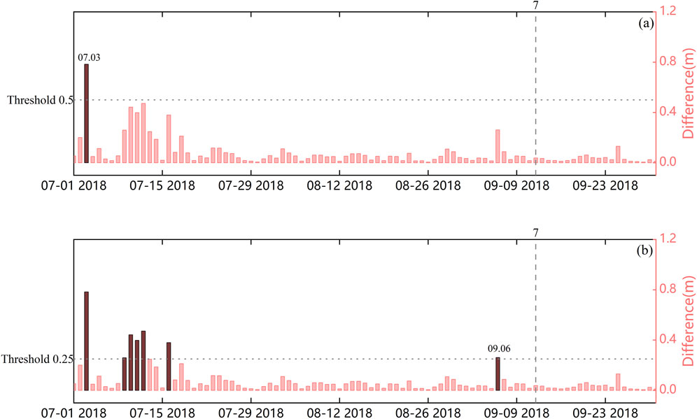
Figure 4. Anomaly judgement of water level differential scores at different thresholds. The red columns are water level differential scores for well C-48, studied over the period 1 July 2018 to 1 October 2018, and seismic 7 is indicated by vertical scribing. A horizontal dotted line denoted the thresholds, while the red bar depicted the differences of the groundwater level, and the differential above the threshold line is the black bar, i.e., the anomaly.

In use, there is no need to manually select a threshold. The Molchan method automatically traverses the cycle from the differential water values maximum to the minimum value, we can obtain multiple sets of v and τ corresponding to the different thresholds. Molchan diagram takes into account the combined results of all thresholds and avoids subjectivity in identifying anomalies.

3.2 Wavelet coherence analysis

Wavelet coherence analysis quantifies the correlation between groundwater level and theoretical tidal series by measuring their temporal relationship (Grinsted et al., 2004; Song et al., 2023; Yang and McCoy, 2023). It identifies resonance periods through phase-shifted arrows in highlighted regions, revealing the degree of correlation between two time series X and Y:

$R^2\left(s\right)=\frac{{\left.\left|S\right.\left(s^{-1}{W}^{XY}\left(s\right)\right)\right|}^2}{\left.S\left(s^{-1}{\left|W^x\left(s\right)\right|}^2\right)*S\left(s^{-1}{\left|W^y\left(s\right)\right|}^2\right)\right)}(3)$

where W^X and W^Y are discrete wavelet transforms, W^XY is the cross wavelet transform of X and Y, S is the smoothing window, and R² is the coherence coefficient. R² is ranging from 0 to 1, with values close to 1 indicating that groundwater levels and tides vary in a high correlated manner. The wavelet coherence coefficient resembles the correlation coefficient in the traditional sense, and it can be understood as a localized correlation coefficient within the frequency space. Simply enter two time series groundwater level and theoretical tide with the same resolution, and R² between them will be calculated according to Equation 3. The code based on MATLAB is already publicly available for download (Grinsted et al., 2004).

3.3 Leaky aquifer model construction

Based on the tidal effect of groundwater level, the Leaky Aquifer Model is used to invert the specific leakage. First, tidal analysis of the water level data facilitates the determination of both observed and theoretical values for various tidal sub-waves’ parameters. In this analysis, two key parameters are the amplitude ratio, which is the observed amplitude divided by the theoretical amplitude, and the phase shift, which represents the difference between the observed phase and the theoretical phase. Both parameters are essential for understanding the tidal analysis. By constructing response models for different well-aquifer systems, the phase shift and amplitude can be utilized to invert the hydraulic parameters of the aquifer.

In situations where the aquifer’s water primarily flows horizontally towards the borehole, a negative phase shift is observed. The radial flow model (Cooper et al., 1965; Hsieh et al., 1987) can be employed to invert the permeability coefficient under these conditions. However, in more realistic scenarios where the aquifer interacts with surrounding rocks through hydraulic processes such as leakage, the phase shift tends to exhibit a leading behavior. The leaky aquifer model can be utilized to derive the specific leakage (σ), expressed as σ = k'/b', where k' and b' represent the permeability coefficient and thickness of the aquitard (Gu et al., 2024; Wang et al., 2018). Significantly, this model also accounts for scenarios where flow within the aquifer is purely radial (k' = 0). The specific leakage (σ) serves as an indicator of the aquitard’s vertical water transport capacity. The theoretical equations of leaky aquifer model are as follows:

$T\left(\frac{{\partial }^{2}h}{\partial r^2}+\frac{1}{r}\frac{\partial h}{\partial r}\right)-\frac{K^{\prime }}{b^{\prime }}h=S\left(\frac{\partial h}{\partial t}-\frac{B{k}_u}{\rho g}\frac{\partial \epsilon }{\partial t}\right)(4)$

where T (m²/s) and S are the transmissivity and storage coefficient of the aquifer, respectively, r is the lateral distance from the well, k and k' are the permeability coefficients of the aquifer and the aquitard, respectively, b and b' are the thicknesses of the two, and B and K_u are the skempton’s coefficient and the undrained bulk modulus, respectively. Equation 4 has the analytical solution as:

$A=abs\left(\frac{i\omega S}{i\omega S+\left(k^{\prime }/b^{\prime }\right)\xi }\right)(5)$

$\eta =\arg \left(\frac{i\omega S}{i\omega S+\left(k^{\prime }/b^{\prime }\right)\xi }\right)(6)$

Where

$\xi =1+{\left(\frac{r_c}{r_{\omega }}\right)}^2\frac{i\omega r_{\omega }{K}_0\left(\beta r_{\omega }\right)}{2T\beta K_1\left(\beta r_{\omega }\right)}(7)$

$\beta =\sqrt{\frac{k^{\prime }}{T{b}^{\prime }}+\frac{i\omega S}{T}}(8)$

where A and η are the tidal parameter amplitude and phase shift, respectively, and r_c and r_ω are the case pipe radius and well filter pipe radius, respectively.

In use, we need to input the known parameters: A, η, r_c, r_ω and Bku, then the specific leakage can be computed by combining Equations 5–8 in MATLAB using open-source code (Zhang et al., 2024).

3.4 Random forest regression

Random forest regression (RFR) was used for sensitivity analysis and was able to quantify the potential contribution of multiple factors to PRI (Borup et al., 2023; Rigatti, 2017). It uses the bootstrap resampling technique to generate a new set of training samples by repeated random sampling of n samples from the original training sample set T. Each independently sampled training sample is used to train a tree, and the n decision trees generated from the sample set are computed in parallel to select the optimal result, which improves the model’s generalization ability. The Gini index is used to complete the establishment of the regression tree, the smaller the Gini index, the better the decision tree division (Breiman, 2001). Assuming that the sample T contains k classes, the Gini coefficient can be expressed as:

$Gini\left(T\right)=1-{\displaystyle \sum _{k=1}^n}{p}_k^2(9)$

where p_k denotes the probability that the sample belongs to the kth class. The smaller the Gini index, the smaller the uncertainty will be and will be more useful for feature testing. After normalizing all the factor series and inputting them into the RFR at the same time as the PRI, the contribution of each type of factor to the PRI will be output. The code is based on MATLAB's own function Treebagger, and the resluts of Equation 9 will automatically calculate (https://ww2.mathworks.cn/help/stats/treebagger.html).

4 Results and discussion

4.1 Quantification of groundwater level changes characteristics before earthquakes

Some studies have reported changes in groundwater levels prior to certain earthquakes (Wang and Manga, 2021), but these observations are not universal or consistent. The mechanisms of such changes remain poorly understood, and currently there is no reliable way to use groundwater level variations as earthquake precursors. Therefore, it is necessary to statistically screen valid anomalies from a large number of suspected anomalies and establish the correspondence between groundwater level anomalies and subsequent earthquakes by the Molchan method. Anomalies are defined in this paper as differences exceeding a certain threshold. In the Molchan method, the threshold is adaptively selected (more details see Section 3.1). The premise of the method: a certain number of samples are needed, the samples include groundwater level and seismic data, and the longer the groundwater level series, the better. In the groundwater level time series, we can identify suspected anomalies, but this may not actually be the case (Figure 3). After accumulating a certain number of suspected anomalies, they are then matched with seismic data occurring in the vicinity. The more samples involved in the calculation, the more accurate the statistical results will be, ultimately revealing the correlation between groundwater level changes and subsequent earthquake events.

Figure 3 shows that pre-processing groundwater level data using differential values effectively highlights anomalies in groundwater levels. These anomalies are mainly marked by notably high values that deviate significantly from the surrounding data points, particularly in the period preceding the earthquake event (Differential values in green circles). Wells C-43, C-42, and C-47 exhibit more anomalies prior to the earthquake, potentially providing clearer indications of seismic activity. In contrast, wells C-05, C-03, and C-48 show no significant groundwater level changes, and the remaining two wells display only general fluctuations. However, subjectivity is not a discriminating criterion, and we will use the Molchan diagram to a further test.

Molchan method unifies the characteristics of groundwater level changes before earthquakes, which provides a quantitative indicator that we defined as pre-response index (PRI). PRI represents the area to the right of the Molchan test line, ranging from 0 to 1.The closer it is to 1, the stronger the correlation between groundwater level changes and subsequent events (Lai et al., 2021; Sun et al., 2017). Figure 5 shows the results of the PRI for eight wells under a 30-day alarm region period. The v-t test lines for wells C-41, C-47, and C-48 are closer to the Gain line of Gain = 2, and grey areas are higher and more significant, indicating a relatively higher PRI. The v-t test lines for wells C-05 are the lowest, falling well below 0.5, indicating that the PRI is relatively lower.

Figure 5

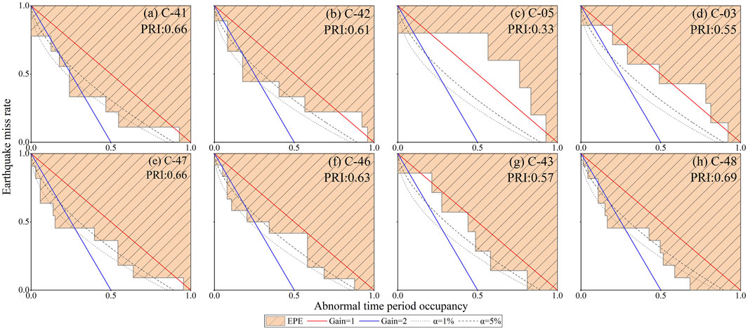
Figure 5. Results of the Molchan test for 8 wells over a 30-day alarm region. The red lines and blue lines show the Gain value. The dashed lines indicate the significance level. Shaded area points to the PRI.

Furthermore, to enhance the precision and reliability of the Molchan test, an assessment of PRI was conducted across various alarm regions, limited to a maximum of 180 days. Figure 6 presents the PRI of eight monitoring wells within this timeframe. Distinct variations in PRI were observed among the wells. The average PRI over a 6-month period ranged from a minimum of 0.35 to a maximum of 0.71, indicating a considerable disparity. Wells C-41, C-43, and C-47 have a good performance in general (PRI of more than 2/3), while the PRI of wells C-03 and C-05 is relatively low (PRI close to 1/3), C-42, C-46 and C-48 show average performance (between 2/3 and 1/3).

Figure 6

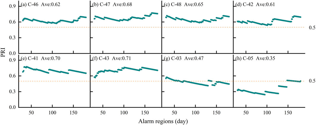
Figure 6. PRI of groundwater levels in 8 wells across different alarm regions (ranging from 1 month to 6 months). The green dots indicate the PRI under different alarm regions. The yellow dotted line denotes the median of PRI.

Despite the similarity in tectonic units and the wells’ location in fractured media aquifers, as well as the comparable distances between the selected earthquakes and the wells, the groundwater level PRI exhibits noticeable variations. These variations provide a unique opportunity to identify factors that govern groundwater level changes before earthquakes.

4.2 Attribution analysis of groundwater level changes characteristics before earthquakes

The aquifer characteristics, particularly the confinement, play a crucial role in determining the wells’ responsiveness to seismic stress. Furthermore, hydraulic parameters significantly influence the magnitude of water level response, thereby affecting the characteristics of groundwater level changes. Tidal effect and seismic static stresses induce certain disturbances within the aquifer and can be considered as “typical representatives” of aquifer response to external stresses. Groundwater levels that exhibit favorable responses to both types of stresses are more likely to demonstrate satisfactory correlations with subsequent earthquakes. Additionally, the distribution of epicenters in relation to the stress propagation path may also influence PRI, serving as an important factor that warrants consideration. In this section, we selected the degree of tidal action experienced by the wells, the co-seismic response magnitude, the hydraulic properties of the aquifer, and the orientation of the epicenter as factors to correlate with PRI. This comprehensive analysis aims to shed light on the factors contributing to the difference of PRI among the monitored wells. The PRI serves as a reliable indicator of the correlation between groundwater level changes and subsequent earthquake events.

This analysis involved multiple steps. First, we evaluated the co-seismic and tidal response coefficients by basic statistics and wavelet coherence analysis, since the role of tides is potentially significant and needs to be treated in the frequency domain to highlight the correlation between the time series. In addition, spectral analysis and leaky aquifer model were utilized to assess the aquifer confinement and hydraulic parameter, both of which are suitable for dealing with periodic signals similar to tidal action. Based on these evaluations, a comparative analysis was performed to assess whether the conditions were responsible for the observed differences in PRI. Secondly, we quantitatively analyzed the impact of the epicenter’s distribution location on the PRI of the wells’ water levels. This analysis aimed to identify any correlations between the spatial distribution of seismic events and the PRI. Lastly, we employed the RFR method to integrate the analyzed factors with the sensitivity analysis of the factors controlling the differences in PRI. This is because it is suitable for multiple series to be analyzed simultaneously with strong robust-ness. This combined analysis aimed to identify the factors that are more likely to contribute to the variations in PRI. Ultimately, our goal was to identify the key factors that significantly impact the variations in PRI.

4.2.1 Influence of co-seismic response and tidal effect

Tidal forces, being a distinct form of crustal stress, often generate long-lasting cyclic variations in well water level. A frequently observed phenomenon is that earthquakes may semi-permanently alter the character of the tidal response (Shi and Wang, 2014; Shi and Wang, 2015). Similarly, seismic events exert static stresses that induce temporary alterations in well water level (Wang and Chia, 2008). Wells that exhibit heightened sensitivity to these common external stresses are expected to display more pronounced responses before earthquakes.

To determine the extent of tidal influence, we quantified the ratio of the time during which water levels were affected by tides to the overall duration of the study period. The relevant rate can be obtained by inputting a tidal sequence and a groundwater level sequence with the same time span and calculating them using Equation 3 The results were presented using the wavelet coherence method, as shown in Figure 7A. Additionally, the degree of co-seismic response was evaluated by calculating the co-seismic response rate Figure 7B, based on the earthquake data from Table 1. This analysis allows us to gauge the wells’ sensitivity to seismic events (Table 3).

Figure 7

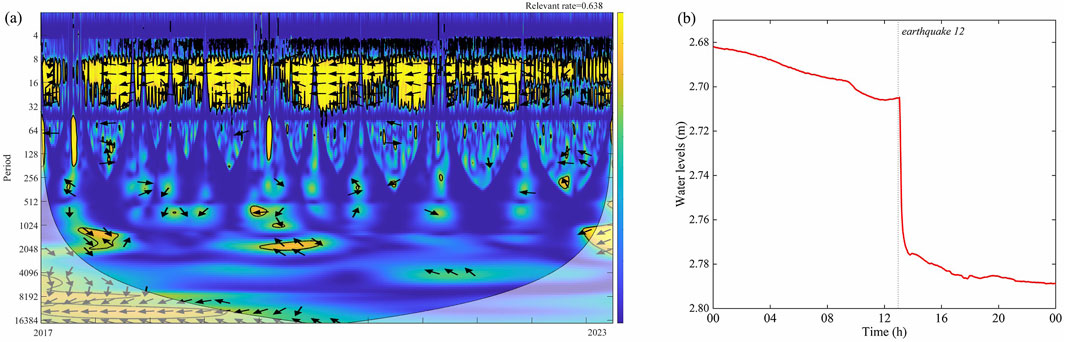
Figure 7. Tidal and co-seismic responses of water levels (A) Wavelet coherence analysis between water levels and tidal effects. The vertical coordinate of the graph represents the period (h), while the horizontal coordinate represents the time (year) Highly correlated regions are highlighted in yellow and those surrounded by a thick black line represent those that passed the Monte Carlo test at a significance level of 5%. Arrows to the right of the graph represent a same-direction alignment, and arrows to the left represents an opposite-direction alignment, and arrows pointing vertically down represents the lead of 90°. (B) co-seismic water level changes. If the water level changes rapidly within a short period of time after an earthquake, it is considered to have a co-seismic effect.

Table 3

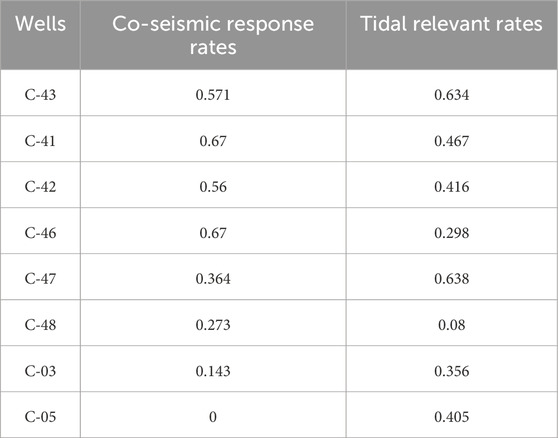
Table 3. Sensitivity of groundwater level in monitoring wells to co-seismic response and tidal effect.

Considering that the Molchan diagram method utilized in this study is based on daily average water level data, the impact of co-seismic events and the persistence of solid tides on PRI are likely to be minimal. Consequently, the statistical results presented in Table 3 are likely to accurately reflect the actual situation. Wells C-41, C-47, and C-43 consistently exhibit superior performance across all stress factors, while wells that perform poorly under one or both stresses tend to have lower PRI. To further investigate the relationship between the degree of stress influence and PRI, a multivariate regression analysis was conducted. The PRI (P) was treated as the dependent variable, while the degree of co-seismic response (C) and the degree of tidal response (T) were considered as independent variables, presupposed to be independent of each other. The resulting binary regression equation derived from this analysis is as follows: P = 0.411C + 0.462T + 0.205. The regression model highlights that higher degrees of co-seismic and tidal responses in the groundwater level are associated with higher PRI. However, it is worth noting that well C-48 deviates from this relationship, possibly due to its location within the fault fracture zone which is more sensitive and vulnerable than the hydraulic properties away from the fault damage zone (Yan et al., 2016; Zhang et al., 2021). This model underscores the notion that wells exhibiting heightened sensitivity to external stresses are more likely to demonstrate superior PRI.

4.2.2 Influence of aquifer confinement

Confined aquifers are generally recognized for their heightened responsiveness to crustal strains, while unconfined aquifers are considered to be less susceptible to strain-induced changes. Leveraging this characteristic, the analysis of groundwater level data in terms of tidal response can serve as a means to distinguish aquifer confinement. The presence of tidal components in the water levels can exhibit inconsistencies that are constrained by the level of well confinement (Bredehoeft, 1967). The groundwater level includes five principal tidal constituents: M2, O1, S2, N2, and K1. These components, with periods close to 12 h and 24 h, account for 95% of the total tidal potential. By analyzing their individual energies, we can infer the degree of confinement of the aquifer (Hu et al., 2024).

We performed a spectral analysis of groundwater levels. To focus on the target frequencies, we excluded those below 0.5 cycles per day (cpd) and frequencies above 2.5 cpd, thereby eliminating the trend term of the water level data. The discrimination of confinement was based on the fact that aquifers with all tidal components and dominated by the M2 component indicate. a certain degree of confinement. In contrast, aquifers with minimal confinement did not contain O1, M2 and N2 (Rahi and Halihan, 2013).

Applying the aforementioned criterion for discrimination, we observed that well C-48 lacks any discernible component waves in its water level, indicating weak confinement characteristics. Similarly, wells C-03 and C-41 exhibit signs of inadequate confinement, as they lack the prominent M2 wave. In contrast, the remaining five wells C-05, C-42, C-43, C-46, C-47 display the highest amplitude for the M2 wave and encompass the presence of other tidal components, which suggests a relatively robust system constraint and a certain degree of aquifer confinement (Figure 8).

Figure 8

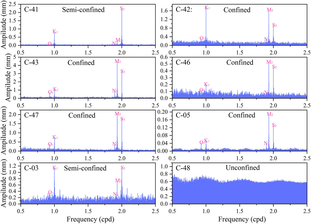
Figure 8. Fast Fourier spectral analysis of water level in 8 Wells. Five main tidal constituents are marked by red.

The correlation analysis conducted between aquifer confinement and PRI reveals unexpected findings. Well C-48, characterized by very poor aquifer confinement, surprisingly exhibits a moderate PRI of 0.65. On the other hand, well C-05, which demonstrates a minimum PRI of 0.35, is deemed to possess good confinement. We also adopted a similar strategy to Hu et al. (2024) by dividing confined, semi-confined, and unconfined into 1, 0.5, and 0 to facilitate PRI comparisons, but still did not find a significant correlation. These results indicate that aquifer confinement may not be the dominant factor influencing changes of groundwater level before earthquakes. Instead, the relationship between confinement and PRI appears to exhibit a certain level of randomness on a smaller scale.

4.2.3 Influence of hydraulic parameters

To determine the hydraulic parameters, we first performed tidal analysis on the water level data using the Baytap08 software (Tamura et al., 1991). The software is now publicly available for download (https://igppweb.ucsd.edu/∼agnew/Baytap/baytap.html). We only need to import the groundwater level series and time series to automatically calculate the relevant tidal parameters. The analysis used a 30-day window and a 15-day step size (Zhang et al., 2021; Zhang et al., 2024). To ensure accuracy, data with significant errors were excluded (Figure 9). The focus was on M2 wave component, which is less affected by baroclinic interference and exhibits a more pronounced amplitude.

Figure 9

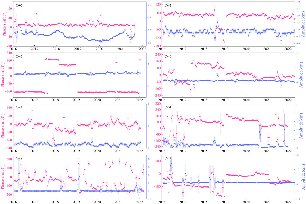
Figure 9. Phase shift and amplitude of M2 calculated using Baytap08 for water level in 8 wells.

Typically, the aquifer’s water is assumed to undergo radial flow, resulting in an expected lag in the phase shift of the water level during tidal analysis. However, the wells selected for this study exhibited a phase ahead during their monitoring periods. This observation suggests that the water level dynamics are influenced not only by radial flow within the aquifer but also by other factors, such as aquifer leakage. In such cases, hydrodynamic exchange with neighboring aquifers in the vertical direction can induce a positive change in the phase shift (Hsieh et al., 1987; Wang et al., 2018). As an illustrative example, well C-46 exhibits a noticeable positive phase shift. This particular well comprises two aquifers characterized by sandstone as the predominant lithology, providing favorable conditions for aquifer leakage (Figure 2). This alignment with theoretical lends support to the observed phase shift. Similarly, well C-05 contains a main aquifer with an overburden aquifer, allowing for geological conditions conducive to leakage, thus aligning with the observed phase shift behavior. By employing appropriate models, these configurations enable the calculation of specific leakage. The distinct variations in phase and amplitude of the water level among wells can be attributed to varying hydraulic parameters. Differences in hydraulic parameters may, in turn, further contribute to divergent levels of PRI.

In summary, there is a suitable condition to calculate the specific leakage using the leaky aquifer model. The phase shift and amplitude ratios obtained from the tidal analysis served as inputs for the model. By employing a 15-day time step, the specific leakages were calculated, providing a comprehensive set of coefficient values for each well throughout the study period. The calculations were visualized in Figure 10, with the long blue bars representing the magnitude of PRI. Bars offer a clear indication of the PRI across the analyzed time frame. A significant correlation is observed between a decrease in PRI and an increase in specific leakage (R² = 0.91). Wells C-43 and C-47, characterized by higher PRI, exhibit relatively smoother specific leakage, converging towards zero. Conversely, the specific leakage values of well C-05 present a notable degree of deviation and dispersion, displaying a broad range of magnitudes. Meanwhile, wells C-42 and C-46 demonstrate a moderately transitional pattern in their specific leakage values, inversely related to their respective PRI. This observed pattern suggests that the specific leakage, as a contributing factor influencing the changes in water volume within the aquifer, plays a crucial role in modulating the sensitivity of the groundwater level to strain. Consequently, this variability in specific leakage contributes to fluctuations in the PRI. Furthermore, previous studies have highlighted the relationship between increased vertical permeability of aquifers and a subsequent rise in local groundwater level and flow rates (Rutter et al., 2016; Wang et al., 2016). The result further supports the notion that discrepancies in hydraulic parameter magnitudes within aquifers, particularly specific leakage, exert a substantial influence on the PRI of water levels in wells. Specific leakage variations may serve as key determinants in the overall PRI of water levels.

Figure 10

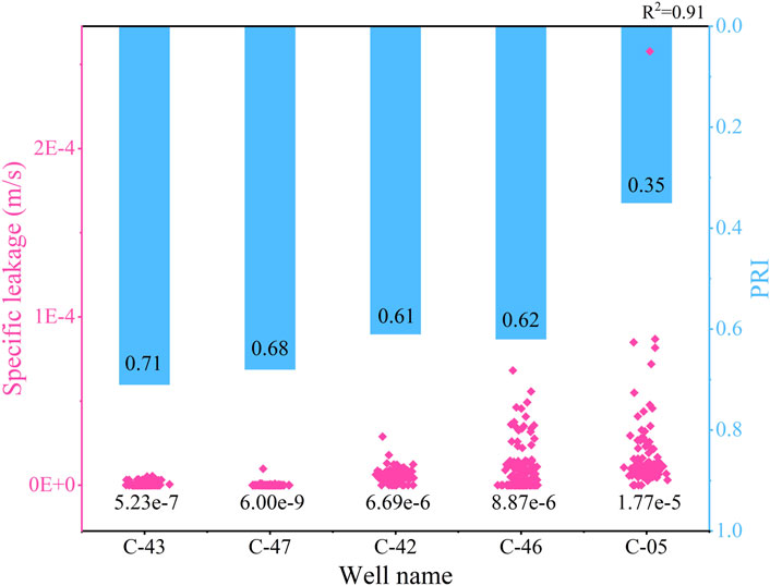
Figure 10. Comparison of well specific leakage and PRI. The long blue bar indicates PRI; the red scatter points denote all specific leakage for different wells at the study timeline, with the mean of specific leakage displayed below. R² = 0.91 refers to the correlation between specific leakage and PRI.

4.2.4 Influence of the epicenter location distribution

Extensive investigations have demonstrated distinct hydrological responses associated with various earthquake parameters, including magnitude, epicenter distance, and seismic energy density (Lai et al., 2016; Weaver et al., 2019). In this subsection, we focus on exploring whether the distribution of epicenter influences the observed disparities in water level PRI.

The Longmenshan-Anninghe fault zone lies between the Tibetan Plateau and the Sichuan Basin, with the 8 selected wells positioned at the intersection of these two geological features. The seismic activity in this vicinity is influenced by the active ruptures occurring in the broader regional context. Thus, the assessment of water level PRI focuses on earthquakes listed in Table 1, categorized based on whether the epicenters align with the Longmenshan-Anninghe fault (as detailed in Table 4). Specifically, the analysis includes earthquakes numbered 2, 7, 8, 10, 11, 12, and 16, which are associated with the target rupture zone.

Table 4

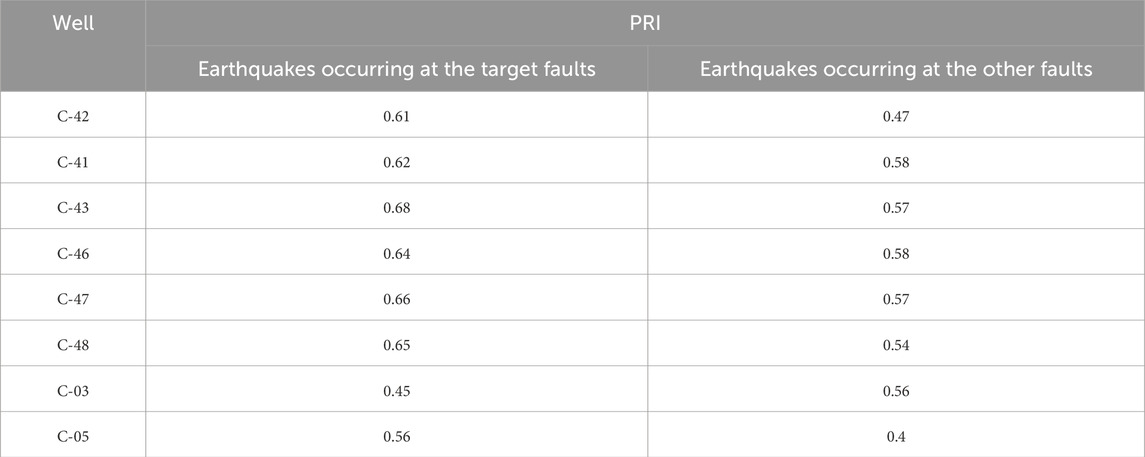
Table 4. Assessment of PRI across different epicenter distributions.

The application of the Molchan test reveals notable disparities in water level among the examined wells, highlighting superior PRI for earthquakes occurring along the target rupture zone. This observed phenomenon may be attributed to the influence of shear stress. Wells exhibiting favorable PRI are positioned between extensive fracture zones and lie within dominant propagation paths of the earthquakes (Brodsky et al., 2020; Freed, 2005). Consequently, wells are subjected to increased tectonic stresses, which may enhance their PRI. Moreover, laboratory studies on rock have shown that stress loading and unloading can significantly alter the permeability of fractured rocks (Ishibashi et al., 2018; Olsson and Barton, 2001). It is likely that the stress changes associated with seismic events interact with the geological structures, thereby affecting the permeability properties of the surrounding rocks. Consequently, variations in PRI can be attributed to the specific distribution patterns of earthquakes and their corresponding impact on the hydrogeological properties around the wells.

4.3 Sensitivity analysis of multiple influencing factors

Hydraulic parameters and seismic distribution can significantly affect the PRI of water level, and the degree of water level response to stress can also reflect the PRI, while the confinement of the aquifer in wells may not have a significant effect on the PRI. In order to identify the relative influence of various factors on the PRI of water level, the sensitivity analysis of these four types of factors was conducted using the RFR. This method effectively integrates both quantitative and qualitative results, and is easy to be combined with the previous analysis. Here, weights in confinement to unconfinement are given as 1, 0.5 and 0, and other relevant factors need to be normalized as well. Then by inputting the series corresponding to each type of factor and PRI, RFR can automatically generate results.

Table 5 presents the weight proportions obtained from the RFR. Among the selected factors, distribution of the earthquakes stands out as the predominant control, exerting a substantial influence on the discrepancies observed in PRI. The hydraulic parameters also contribute to the variations in water level PRI, but with a weightage that is only slightly lower than the distribution of the earthquakes. In contrast, the degree of water level response to external stress (Tidal effects and Co-seismic responses) and the confinement conditions of the aquifer exhibits comparatively weaker impacts on PRI, as indicated by their lower weightages, indicating their relatively lesser significance in determining the PRI of water level.

Table 5

Table 5. Sensitivity calculations of factors influencing PRI by RFR.

In our selected cluster of wells, C-46, C-42, and C-48 exhibiting moderate PRI in comparison to the remaining wells. These three wells are situated at the intersection of the Longmenshan-Anninghe faults, thus are significantly affected by the distribution of earthquakes because seismic signals are more likely to propagate near the rupture zone, but our screening conditions for seismic events are not oriented. If earthquakes do not occur near the target faults, potential earthquake precursor information is just as easily lost.

Furthermore, differences between wells C-41, C-43, and C-47, characterized by high PRI, and wells C-05 and C-03, identified as having poor PRI, can largely be attributed to the differences in hydraulic parameters of the aquifer, since most of which are located far from faults intersections. The specific leakages differ by 2–3 orders of magnitude, as confirmed in the previous section.

The sensitivity of water level to external stresses (Tidal effects and Co-seismic responses) also offers some insights into PRI, although it is as a secondary criterion. In this regard, the contrasting performance of excellently responding well C-43 compared to wells C-05 and C-03 underscores the potential influence of stress sensitivity on PRI, and can be a useful reflection of the overall expected performance of the well. In our selected wells, the aquifer confinement on PRI shows some randomness, and it may show correlation on a larger scale, so our results conclude that confinement is not enough of a key cue for high or low PRI.

Furthermore, additional factors such as well depth, borehole radius, and the height of the water column within the well should be considered, as they may potentially contribute to variations in PRI. However, their impact on water level PRI is relatively minor. For instance, the slight differences in PRI between wells C-41 and C-43, which have having similar PRI, or among wells C-46, C-48, and C-42, where the difference in PRI varies only slightly within a range of 0.05, illustrate the limited impact of these factors. Although these factors can be relevant in certain scenarios, their overall contribution to altering water level PRI remains secondary in comparison to the dominant factors previously discussed. Hence, the factors affecting the disparities in PRI, ranked in descending order of sensitivity, encompass 1) distribution of the earthquakes in relation to well locations, 2) hydraulic parameters and 3) the sensitivity of water level to external stress responses.

5 Conclusion

We used the Molchan diagram method to quantitatively represent the characteristics of groundwater level changes before an earthquake using pre-response index (PRI). The closer the PRI is to 1, the higher the correlation between water level changes and subsequent events. Over the semi-annual alarm regions, it was observed that wells C-41, C-43, and C-47 exhibited high PRI, while wells C-03 and C-05 displayed low PRI. Meanwhile, the PRI of wells C-42, C-46, and C-48 were found to be of moderate magnitude. Correlation analysis and RFR methods identify the factors influencing the PRI: distribution of the earthquakes in relation to well locations, hydraulic parameters and the sensitivity of water level to external stress responses. In the well water levels studied, we suggest that differences in the distribution of the earthquakes in relation to well locations most favor the variation in PRI. Conversely, the confinement conditions of the aquifer were found to have an insignificant impact on PRI.

Our study data are mainly based on calculations of extensions over observed water levels, additional data used in the article for correlation and sensitivity analyses can be used to derive more precise values from field measurements or expeditions: e.g., hydraulic parameters, confinement, etc. This would be a better balance of accuracy and hopefully further contrast with our study.

Data availability statement

The original contributions presented in the study are included in the article/supplementary material, further inquiries can be directed to the corresponding author.

Author contributions

WZ: Conceptualization, Methodology, Software, Visualization, Writing–original draft. ML: Conceptualization, Funding acquisition, Supervision, Validation, Writing–review and editing. YY: Investigation, Resources, Supervision, Writing–review and editing. XR: Investigation, Resources, Writing–review and editing. ML: Data curation, Visualization, Writing–review and editing. SL: Methodology, Supervision, Writing–review and editing.

Funding

The author(s) declare that financial support was received for the research, authorship, and/or publication of this article. This research was funded by National Natural Science Foundation of China (grant number 42372282), Beijing Natural Science Foundation (grant number 8222003) and National Natural Science Foundation of China (grant number 41877205).

Conflict of interest

The authors declare that the research was conducted in the absence of any commercial or financial relationships that could be construed as a potential conflict of interest.

Generative AI statement

The author(s) declare that no Generative AI was used in the creation of this manuscript.

Publisher’s note

All claims expressed in this article are solely those of the authors and do not necessarily represent those of their affiliated organizations, or those of the publisher, the editors and the reviewers. Any product that may be evaluated in this article, or claim that may be made by its manufacturer, is not guaranteed or endorsed by the publisher.

References

Bai, Y., Huayong, N., and Hua, G. (2019). Advances in research on the geohazard effect of active faults on the southeastern margin of the Tibetan Plateau. J. Geomechanics 25 (6), 1116–1128. doi:10.12090/j.issn.1006-6616.2019.25.06.095

CrossRef Full Text | Google Scholar

Barberio, M. D., Gori, F., Barbieri, M., Billi, A., Caracausi, A., De Luca, G., et al. (2020). New observations in Central Italy of groundwater responses to the worldwide seismicity. Sci. Rep. 10 (1), 17850. doi:10.1038/s41598-020-74991-0

PubMed Abstract | CrossRef Full Text | Google Scholar

Borup, D., Christensen, B. J., Mühlbach, N. S., and Nielsen, M. S. (2023). Targeting predictors in random forest regression. Int. J. Forecast. 39 (2), 841–868. doi:10.1016/j.ijforecast.2022.02.010

CrossRef Full Text | Google Scholar

Bredehoeft, J. D. (1967). Response of well-aquifer systems to Earth tides. J. Geophys. Res. 72 (12), 3075–3087. doi:10.1029/JZ072i012p03075

CrossRef Full Text | Google Scholar

Breiman, L. (2001). Random forests. Mach. Learn. 45, 5–32. doi:10.1023/a:1010933404324

CrossRef Full Text | Google Scholar

Brodsky, E. E., Mori, J. J., Anderson, L., Chester, F. M., Conin, M., Dunham, E. M., et al. (2020). The state of stress on the fault before, during, and after a major earthquake. Annu. Rev. Earth Planet. Sci. 48, 49–74. doi:10.1146/annurev-earth-053018-060507

CrossRef Full Text | Google Scholar

Chen, C.-H., Tang, C.-C., Cheng, K.-C., Wang, C. H., Wen, S., Lin, C. H., et al. (2015). Groundwater–strain coupling before the 1999 Mw 7.6 Taiwan Chi-Chi earthquake. J. Hydrology 524, 378–384. doi:10.1016/j.jhydrol.2015.03.006

CrossRef Full Text | Google Scholar

Cooper, H. H., Bredehoeft, J. D., Papadopulos, I. S., and Bennett, R. R. (1965). The response of well-aquifer systems to seismic waves. J. Geophys. Res. 70 (16), 3915–3926. doi:10.1029/JZ070i016p03915

CrossRef Full Text | Google Scholar

Del Gaudio, E., Stevenazzi, S., Onorati, G., and Ducci, D. (2024). Changes in geochemical and isotopic contents in groundwater before seismic events in Ischia Island (Italy). Chemosphere 349, 140935. doi:10.1016/j.chemosphere.2023.140935

PubMed Abstract | CrossRef Full Text | Google Scholar

Freed, A. M. (2005). Earthquake triggering by static, dynamic, and postseismic stress transfer. Annu. Rev. Earth Planet. Sci. 33, 335–367. doi:10.1146/annurev.earth.33.092203.122505

CrossRef Full Text | Google Scholar

Granin, N. G., Radziminovich, N. A., De Batist, M., Makarov, M. M., Chechelnitcky, V. V., Blinov, V. V., et al. (2018). Lake Baikal's response to remote earthquakes: lake-level fluctuations and near-bottom water layer temperature change. Mar. Petroleum Geol. 89, 604–614. doi:10.1016/j.marpetgeo.2017.10.024

CrossRef Full Text | Google Scholar

Grinsted, A., Moore, J. C., and Jevrejeva, S. (2004). Application of the cross wavelet transform and wavelet coherence to geophysical time series. Nonlinear Process. Geophys. 11 (5/6), 561–566. doi:10.5194/npg-11-561-2004

CrossRef Full Text | Google Scholar

Gu, H., Xu, Y., Lan, S., Yue, M., Wang, M., and Sauter, M. (2024). Spatial variation of aquifer permeability in the North China Plain from large magnitude earthquake signals. Pure Appl. Geophys. 181, 1845–1858. doi:10.1007/s00024-024-03511-2

CrossRef Full Text | Google Scholar

Hattori, K., and Han, P. (2018). “Statistical analysis and assessment of ultralow frequency magnetic signals in Japan as potential earthquake precursors,” in Pre-earthquake processes: a multidisciplinary approach to earthquake prediction studies, 229–240. doi:10.1002/9781119156949.ch13

CrossRef Full Text | Google Scholar

He, H., and Ikeda, Y. (2007). Faulting on the anninghe fault zone, southwest China in late quaternary and its movement model. Acta Seismol. Sin. 29 (5), 571–583. doi:10.1007/s11589-007-0571-4

CrossRef Full Text | Google Scholar

Hsieh, P. A., Bredehoeft, J. D., and Farr, J. M. (1987). Determination of aquifer transmissivity from Earth tide analysis. Water Resour. Res. 23 (10), 1824–1832. doi:10.1029/WR023i010p01824

CrossRef Full Text | Google Scholar

Hu, C., Liao, X., Shi, Y., Liu, C., Yan, R., Lian, X., et al. (2024). Comprehensive quantitative determination of aquifer confinement based on tidal response of well water level and its application in North China. Sci. Rep. 14 (1), 9464. doi:10.1038/s41598-024-59909-4

PubMed Abstract | CrossRef Full Text | Google Scholar

Ishibashi, T., Elsworth, D., Fang, Y., Riviere, J., Madara, B., Asanuma, H., et al. (2018). Friction-stability-permeability evolution of a fracture in granite. Water Resour. Res. 54 (12), 9901–9918. doi:10.1029/2018WR022598

CrossRef Full Text | Google Scholar

Kopylova, G., and Boldina, S. (2020). Hydrogeological earthquake precursors: a case study from the Kamchatka peninsula. Front. Earth Sci. 8, 576017. doi:10.3389/feart.2020.576017

CrossRef Full Text | Google Scholar

Lai, G., Jiang, C., Han, L., Sheng, S., and Ma, Y. (2016). Co-seismic water level changes in response to multiple large earthquakes at the LGH well in Sichuan, China. Tectonophysics 679, 211–217. doi:10.1016/j.tecto.2016.04.047

CrossRef Full Text | Google Scholar

Lai, G., Jiang, C., Wang, W., Han, L., and Deng, S. (2021). Correlation between the water temperature and water level data at the Lijiang well in Yunnan, China, and its implication for local earthquake prediction. Eur. Phys. J. Special Top. 230 (1), 275–285. doi:10.1140/epjst/e2020-000255-3

CrossRef Full Text | Google Scholar

Molchan, G. (1990). Strategies in strong earthquake prediction. Phys. Earth Planet. Interiors 61 (1-2), 84–98. doi:10.1016/0031-9201(90)90097-H

CrossRef Full Text | Google Scholar

Olsson, R., and Barton, N. (2001). An improved model for hydromechanical coupling during shearing of rock joints. Int. J. rock Mech. Min. Sci. 38 (3), 317–329. doi:10.1016/S1365-1609(00)00079-4

CrossRef Full Text | Google Scholar

Pulinets, S., Ouzounov, D., Karelin, A., and Davidenko, D. (2018). “Lithosphere-atmosphere-ionosphere-magnetosphere coupling-A concept for pre-earthquake signals generation,” in Pre-earthquake processes: a multidisciplinary approach to earthquake prediction studies. Editors D. Ouzounov, S. Pulinets, K. Hattori, and P. Taylor, 234, 79–98.

Google Scholar

Rahi, K. A., and Halihan, T. (2013). Identifying aquifer type in fractured rock aquifers using harmonic analysis. Ground Water 51 (1), 76–82. doi:10.1111/j.1745-6584.2012.00925.x

PubMed Abstract | CrossRef Full Text | Google Scholar

Rigatti, S. J. (2017). Random forest. J. Insur. Med. 47 (1), 31–39. doi:10.17849/insm-47-01-31-39.1

PubMed Abstract | CrossRef Full Text | Google Scholar

Roeloffs, E., Quilty, E., and Scholtz, C. H. (1997). Case 21: water level and strain changes preceding and following the August 4, 1985 Kettleman Hills, California, earthquake. Pure Appl. Geophys. 149 (1), 21–60. doi:10.1007/bf00945160

CrossRef Full Text | Google Scholar

Rutter, H., Cox, S., Dudley Ward, N., and Weir, J. J. (2016). Aquifer permeability change caused by a near-field earthquake, C anterbury, N ew Z ealand. Water Resour. Res. 52 (11), 8861–8878. doi:10.1002/2015WR018524

CrossRef Full Text | Google Scholar

Shi, Z., and Wang, G. (2014). Hydrological response to multiple large distant earthquakes in the Mile well, China. J. Geophys. Res. Earth Surf. 119 (11), 2448–2459. doi:10.1002/2014jf003184

CrossRef Full Text | Google Scholar

Shi, Z., and Wang, G. (2015). Sustained groundwater level changes and permeability variation in a fault zone following the 12 May 2008, Mw 7.9 Wenchuan earthquake. Hydrol. Process. 29 (12), 2659–2667. doi:10.1002/hyp.10387

CrossRef Full Text | Google Scholar

Shi, Z., Wang, G., and Liu, C. (2013). Co-seismic groundwater level changes induced by the May 12, 2008 Wenchuan earthquake in the near field. Pure Appl. Geophys. 170, 1773–1783. doi:10.1007/s00024-012-0606-1

CrossRef Full Text | Google Scholar

Song, C., Chen, X., and Xia, W. (2023). Improving the understanding of the influencing factors on sea level based on wavelet coherence and partial wavelet coherence. J. Oceanol. Limnol. 41 (5), 1643–1659. doi:10.1007/s00343-022-2102-5

CrossRef Full Text | Google Scholar

Sun, X., Xiang, Y., Shi, Z., and Wang, B. (2017). Preseismic changes of water temperature in the yushu well, western China. Pure Appl. Geophys. 175 (7), 2445–2458. doi:10.1007/s00024-017-1579-x

CrossRef Full Text | Google Scholar

Sun, X.-L., Wang, G.-C., and Yan, R. (2016). Extracting high-frequency anomaly information from fluid observational data: a case study of the Wenchuan Ms8.0 earthquake of 2008. Chin. J. Geophys. 59 (5). doi:10.6038/cjg20160512

CrossRef Full Text | Google Scholar

Tamura, Y., Sato, T., Ooe, M., and Ishiguro, M. (1991). A procedure for tidal analysis with a Bayesian information criterion. Geophys. J. Int. 104 (3), 507–516. doi:10.1111/j.1365-246x.1991.tb05697.x

CrossRef Full Text | Google Scholar

Wang, C. y., and Chia, Y. (2008). Mechanism of water level changes during earthquakes: near field versus intermediate field. Geophys. Res. Lett. 35 (12). doi:10.1029/2008gl034227

PubMed Abstract | CrossRef Full Text | Google Scholar

Wang, C. Y., Doan, M. L., Xue, L., and Barbour, A. J. (2018). Tidal response of groundwater in a leaky aquifer—application to Oklahoma. Water Resour. Res. 54 (10), 8019–8033. doi:10.1029/2018wr022793

CrossRef Full Text | Google Scholar

Wang, C. Y., Liao, X., Wang, L. P., and Manga, M. (2016). Large earthquakes create vertical permeability by breaching aquitards. Water Resour. Res. 52 (8), 5923–5937. doi:10.1002/2016WR018893

CrossRef Full Text | Google Scholar

Wang, C.-Y., and Manga, M. (2021). Water and earthquakes. Springer Nature.

Google Scholar

Wang, K., Chen, Q.-F., Sun, S., and Wang, A. (2006). Predicting the 1975 Haicheng earthquake. Bull. Seismol. Soc. Am. 96 (3), 757–795. doi:10.1785/0120050191

CrossRef Full Text | Google Scholar

Weaver, K., Doan, M. L., Cox, S., Townend, J., and Holden, C. (2019). Tidal behavior and water-level changes in gravel aquifers in response to multiple earthquakes: a case study from New Zealand. Water Resour. Res. 55 (2), 1263–1278. doi:10.1029/2018wr022784

CrossRef Full Text | Google Scholar

Yan, R., Tian, L., Wang, G., Zhong, J., Liu, J., and Zhou, Z. (2018). Review and statistically characteristic analysis of underground fluid anomalies prior to the 2008 Wenchuan Ms8.0 earthquake. Chin. J. Geophys. 61 (5), 1907–1921. doi:10.6038/cjg2018M0162

CrossRef Full Text | Google Scholar

Yan, R., Wang, G., and Shi, Z. (2016). Sensitivity of hydraulic properties to dynamic strain within a fault damage zone. J. Hydrology 543, 721–728. doi:10.1016/j.jhydrol.2016.10.043

CrossRef Full Text | Google Scholar

Yang, G., and McCoy, K. (2023). Modeling groundwater-level responses to multiple stresses using transfer-function models and wavelet analysis in a coastal aquifer system. J. Hydrology 627, 130426. doi:10.1016/j.jhydrol.2023.130426

CrossRef Full Text | Google Scholar

Yi, G., Xueze, W., Jun, F., and Wang, S. w. (2004). Assessing current faulting behaviors and seismic risk of the Anninghe-Zemuhe fault zone from seismicity parameters. Acta Seismol. Sin. 17, 322–333. doi:10.1007/s11589-004-0054-9

CrossRef Full Text | Google Scholar

Zechar, J. D., and Jordan, T. H. (2008). Testing alarm-based earthquake predictions. Geophys. J. Int. 172 (2), 715–724. doi:10.1111/j.1365-246X.2007.03676.x

CrossRef Full Text | Google Scholar

Zhang, H., Shi, Z., Wang, G., Yan, X., Liu, C., Sun, X., et al. (2021). Different sensitivities of earthquake-induced water level and hydrogeological property variations in two aquifer systems. Water Resour. Res. 57 (5), e2020WR028217. doi:10.1029/2020WR028217

CrossRef Full Text | Google Scholar

Zhang, P.-Z. (2008). The tectonic deformation,strain distribution and deep dynamic processes in the eastern margin of the Tibetan Plateau. Sci. China Ser. D-Earth Sci. Chin. 38 (9), 1041–1056. doi:10.3321/j.issn:1006-9267.2008.09.001

CrossRef Full Text | Google Scholar

Zhang, P.-Z., Xu, X.-W., Wen, X.-Z., and Ran, Y.-K. (2008). Slip rates and recurrence intervals of the Longmen Shan active fault zone and tectonic implications for the mechanism of the May 12 Wenchuan earthquake, 2008, Sichuan, China. Chin. J. Geophys. 51 (4), 1066–1073 doi:10.3321/j.issn:0001-5733.2008.04.015

CrossRef Full Text | Google Scholar

Zhang, S., Shi, Z., Wang, G., Zhang, Z., and Guo, H. (2023). The origin of hydrological responses following earthquakes in a confined aquifer: insight from water level, flow rate, and temperature observations. Hydrology Earth Syst. Sci. 27 (2), 401–415. doi:10.5194/hess-27-401-2023

CrossRef Full Text | Google Scholar

Zhang, Y., Manga, M., Fu, L. Y., Zhang, H., Huang, T., Yang, Q., et al. (2024). Long-and short-term effects of seismic waves and coseismic pressure changes on fractured aquifers. J. Geophys. Res. Solid Earth 129 (3), e2023JB027970. doi:10.1029/2023jb027970

CrossRef Full Text | Google Scholar