A simplified 3D finite difference method for electromagnetic logging while drilling simulation in symmetrical models

Electromagnetic (EM) Logging While Drilling (LWD) plays an increasingly significant role in oil and gas exploration and development. Fast and accurate simulation of EM LWD is essential for optimizing tool parameters and data processing. As the depth of investigation increases, EM LWD simulation and inversion in complex geological structures become more important, while the computational cost of three-dimensional (3D) simulations remains a major challenge. In this paper, we present a simplified 3D finite-difference frequency domain method for symmetric geological models. In such models, the electromagnetic field generated by a magnetic dipole source exhibits symmetry in all directions. Leveraging this symmetry, we reduce the computational domain by half, centering it on the symmetry plane, and impose new boundary conditions based on the symmetry of the electric field. Compared to conventional methods, the proposed approach reduces the number of unknowns by half, significantly improving computational efficiency. Numerical simulations show that the results from the proposed method agree well with both analytical solutions and finite element simulations. We further apply the method to analyze borehole effects, mud invasion, and near-wellbore anomalies. The numerical results indicate that in a 12-inch diameter borehole, EM LWD apparent resistivity curves are influenced by borehole effects, deviating from those obtained under borehole-free conditions. The impact of the borehole and mud invasion varies with tool frequency and transmitter-receiver (TR) spacing: shorter TR spacings and higher frequencies are more susceptible to these effects, whereas longer TR spacings and lower frequencies exhibit greater stability.

1 Introduction

With the increasing number of high angle and horizontal wells, Electromagnetic Logging While Drilling (EM LWD) is widely applied in oil and gas exploration and development (Qin et al., 2017). EM LWD can measure the formation’s electrical properties in real time, allowing for inversion-based determination of formation structures (Pardo and Torres-Verdín, 2015; Li H. et al., 2020). Consequently, it plays a crucial role in horizontal well landing and real-time geosteering (Bittar et al., 2009; Wu B. et al., 2022; Yue et al., 2022). Over the past decades, EM LWD technology has continuously evolved in its applications (Tian et al., 2023). From the perspective of tool structure and detection capabilities, EM LWD has developed from single-frequency and single transmitter-receiver spacing to multi-frequency and multi-spacing configurations (Bittar et al., 1993). Measurement components have expanded from a single coaxial component to multiple components, and the detection depth has increased from several inches to several tens of meters (Bazara et al., 2016; Clegg et al., 2022). In this process, numerical simulation technology has also played an important role (Gao et al., 2010; Qin et al., 2021).

Numerical simulation serves as the foundational basis for the optimization of EM LWD tool parameters, analysis of logging response characteristics, investigation of influencing factors, and data inversion (Wei et al., 2024). To achieve this, a variety of numerical simulation methods have been employed to calculate EM LWD responses (Liu et al., 2015). Depending on the specific requirements, different methods are employed for EM LWD simulation. For conventional EM LWD measurements, the mapping relationship between formation resistivity and phase shift or amplitude ratio can be simulated using the analytical expression of the electromagnetic field generated by a dipole source in a homogenous medium. To further analyze the impact of formation boundaries on the logging response, a pseudo-analytical algorithm in a one-dimensional (1D) model is required (Hong et al., 2016; Li Y. et al., 2020; Wang L. et al., 2020). By combining specific tool signals and inversion algorithms, it becomes possible to obtain formation resistivity and delineate formation boundaries (Wang et al., 2018; Xu et al., 2023). To address the analysis of more complex formation properties, Davydycheva et al. derived a pseudo-analytical algorithm for biaxial anisotropic media (Davydycheva et al., 2014; Fan et al., 2019). As the tool’s detection depth increases, using only a 1D model becomes insufficient to describe the actual formation environment. Therefore, 2.5D algorithms for two-dimensional formation models have been widely applied (Wu et al., 2020b). Chen et al. introduced the 2.5D algorithm into EM LWD simulation and analyzed the impact of faults on the azimuthal EM LWD responses (Chen et al., 2011; Noh et al., 2022). Tool responses in anisotropic and complex scenarios are also discussed with 2.5D algorithms (Zeng et al., 2018; Wu et al., 2020a; Wu Z. et al., 2022).

Recently, to more accurately characterize reservoir structures, 3D inversion has been incorporated into EM LWD measurements and has gradually emerged as a new trend. Consequently, 3D numerical forward modeling has become increasingly essential. In fact, the application of 3D numerical algorithm techniques in EM LWD forward modeling has a long history (Wang and Fang, 2001; Davydycheva et al., 2003). In 3D numerical simulation algorithms, the finite difference method, including the finite difference time domain (FDTD) and finite difference frequency domain (FDFD) methods, is among the most widely used (Lee and Teixeira, 2010; Yuan et al., 2011; Sun and Hu, 2022). It is often applied to simulate and analyze the eccentric response of azimuthal EM LWD tools (Hue et al., 2005; Li and Wang, 2016). As another important numerical simulation method, the finite element method (FEM) offers significant advantages in simulating complex structural models due to its flexible mesh discretization (Jaysaval et al., 2016). In recent years, the discontinuous Galerkin (DG) finite element techniques have also been applied to EM logging simulations (Sun et al., 2017; Zhang et al., 2020). In addition, the finite volume method (FVM) is widely used for simulating the responses of extra-deep EM LWD tools and plays an important role in 3D inversion (Clegg et al., 2019; Wang H. et al., 2020; Wang et al., 2023). Overall, 3D numerical simulation techniques have been effectively applied in EM LWD modeling. This paper focuses on improving the traditional finite difference algorithm for a specific symmetric model to enhance computational efficiency.

In this paper, we apply the 3D finite difference frequency domain method to EM LWD simulation. For symmetric models, a simplified 3D simulation scheme is obtained by applying appropriate boundary conditions. The remainder of this paper is organized as follows. In Section 2, we briefly introduce the physics of EM LWD tools. In Section 3, the 3D finite difference algorithm with symmetric boundary conditions and the difference scheme are presented. In Section 4, the algorithm is validated through comparison with results from other methods. In Section 5, we apply the algorithm to Electromagnetic Logging While Drilling modeling and analyze the effects of borehole and mud invasion on the logging response.

2 Physics of the EM LWD tools

Electromagnetic Logging While Drilling tools were initially designed with a single-transmitter, dual-receiver configuration, using the phase shift and amplitude ratio of the induced electromotive force between two receiver coils to measure formation resistivity. The latest generation of EM LWD tools measures multi-component magnetic fields and employs low frequencies and extended transmitter-receiver spacing to enable formation detection over distances of several tens of meters (Li et al., 2020). Figure 1 shows the basic structure of EM LWD tools. The figure illustrates the tri-axial configuration for both transmitter and receiver. However, in practice, the actual tools may only use a subset of these coil systems, depending on the specific requirements, measuring only a few components. For example, traditional EM LWD tools typically use coaxial coils to measure the H_zz component, while azimuthal EM LWD tools also measure the H_xz/H_zx components. Additionally, some tools utilize tilted coils instead of orthogonal coils to obtain cross-coupling components. It is important to note that actual tools may incorporate additional coil systems and employ multiple frequencies for measurement.

Figure 1

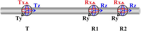
Figure 1. Configuration of typical EM LWD tools.

For traditional EM LWD tools, the basic structure consists of an axial transmitter and two axial receivers. The phase shift (PS) and amplitude ratio (AR) between the dual receiver coils are formally defined by Equations 1, 2, respectively:

$PS=\mathit{atan}\left(\frac{Imag\left(V2\right)}{Real\left(V2\right)}\right)-\mathit{atan}\left(\frac{Imag\left(V1\right)}{Real\left(V1\right)}\right)(1)$

$AR=20\mathit{lg}{\left(\frac{{Imag\left(V1\right)}^2+{Real\left(V1\right)}^2}{{Imag\left(V2\right)}^2+{Real\left(V2\right)}^2}\right)}^{\mathbf{1}/\mathbf{2}}(2)$

where PS and AR represent the phase shift and amplitude ratio between the two receivers, respectively. V1 and V2 are the induced electromotive forces on receiver coil 1 (R1) and receiver coil 2 (R2), respectively. Imag (·) and Real(·) are functions that extract the imaginary and real parts of a complex number, respectively. For azimuthal EM LWD tools, the basic structure is typically single-transmitter, single-receiver. When different tool configurations are used, the definition of the geosignal may vary. For instance, when an orthogonal coil system is employed, the geosignal can be defined as V_zx or V_xz. In contrast, when a tilted coil system is used (Bittar, 2000), the geosignal is defined as the phase shift geosignal (GeoP) and the amplitude ratio geosignal (GeoA). The definitions of GeoP (GeoA) are analogous to those of PS (AR), with the distinction that V1 and V2 no longer represent the induced electromotive forces from the two receiver coils. Instead, V1 and V2 correspond to the induced electromotive forces at tool rotation angles of 0° and 180°, respectively. For extra-deep EM LWD tools, the basic unit is typically a single-transmitter, single-receiver configuration. The measured coaxial, coplanar, and cross components are then used for signal synthesis. Taking Schlumberger’s Geosphere service as an example, its synthesized signals include eight modes: USDA, USDP, UADA, UADP, UHRA, UHRP, UHAA, and UHRP (Seydoux et al., 2014; Wu et al., 2018; Zhang et al., 2021).

3 3D finite difference algorithm

3.1 Governing equation and boundary condition

In EM LWD measurements, fixed frequencies are typically used. In this paper, the time convention of e^-iωt is assumed, and the variation in rock magnetic permeability is ignored. The Maxwell equations in the frequency domain for inhomogeneous medium can be expressed as

$\nabla \times \mathbf{E}=\mathrm{i}\omega {\mu }_0\mathbf{H}(3)$

$\nabla \times \mathbf{H}={\mathrm{J}}_s+\left(\sigma -\mathrm{i}\omega \epsilon \right)\mathbf{E}(4)$

where, E is the Electric field, V; H is the magnetic fields, A⋅m⁻¹; ω is the angular frequency, rad⋅s⁻¹; J_s is the current source, A⋅m⁻²; $\mathit{\sigma }$ is the conductivity tensor, S⋅m⁻¹; μ₀ is the permeability of vacuum, 4π⋅10⁻⁷ H⋅m⁻¹; $\mathit{\epsilon }$ is the dielectric constant, F⋅m^-1. By combining Equations 3, 4, the wave equation of electric field can be obtained as shown in Equation 5. Moreover, the conductivity-permittivity coupling term (σ − iωε) can exhibit anisotropic properties, as characterized in Equation 7.

$\nabla \times \nabla \times \mathbf{E}={\mathrm{i}\omega {\mu }_0\mathbf{J}}_{\mathit{s}}+\mathrm{i}\omega {\mu }_0\left(\sigma -\mathrm{i}\omega \epsilon \right)\mathbf{E}(5)$

The electromagnetic fields generated in the formation is the superposition of the incident field produced by a magnetic dipole source and the scattered field. Specifically, in a homogeneous isotropic formation, only the incident field, denoted as Eⁱ, exists. The scattered field, denoted as E^s, is due to the heterogeneity of the formation. Therefore, the total field can be expressed as the sum of Eⁱ and E^s. Substitute the total field E and the incident field Eⁱ into Equation 3 and take the difference to obtain Equation 6:

$\nabla \times \nabla \times {\mathbf{E}}^{\mathrm{s}}-\mathrm{i}\omega {\mu }_0\widehat{\sigma }{\mathbf{E}}^{\mathrm{s}}=\mathrm{i}\omega {\mu }_0\left(\widehat{\sigma }-{\widehat{\sigma }}_0\right){\mathbf{E}}^{\mathrm{i}}(6)$

where

$\sigma -\mathrm{i}\omega \epsilon =\left[\begin{array}{ccc}{\sigma }_{xx}-\mathrm{i}\omega {\epsilon }_{xx}& {\sigma }_{xy}-\mathrm{i}\omega {\epsilon }_{xy}& {\sigma }_{xz}-\mathrm{i}\omega {\epsilon }_{xz}\\ {\sigma }_{yx}-\mathrm{i}\omega {\epsilon }_{yx}& {\sigma }_{yy}-\mathrm{i}\omega {\epsilon }_{yy}& {\sigma }_{yz}-\mathrm{i}\omega {\epsilon }_{yz}\\ {\sigma }_{zx}-\mathrm{i}\omega {\epsilon }_{zx}& {\sigma }_{zy}-\mathrm{i}\omega {\epsilon }_{zy}& {\sigma }_{zz}-\mathrm{i}\omega {\epsilon }_{zz}\end{array}\right](7)$

Since subsurface rocks are often lossy media, the electromagnetic field will decay to zero far from the source. Therefore, the boundary condition of the EM LWD modeling problem becomes Equation 8:

${\left.\mathit{E}\right|}_{\left(x\to \infty ,or,y\to \infty ,or,z\to \infty \right)}=0(8)$

In fact, considering the exponential decay of the electromagnetic field, using a Perfect Electric Conductor (PEC) boundary at a distance greater than 2.3 times the skin depth from the magnetic dipole source ensures that the boundary’s influence on the simulation results is less than 1%.

3.2 Model construction and conductivity equivalence

Taking into account factors such as the borehole condition, mud invasion and formation structure, a three-dimensional model as shown in Figure 2 is established. For the three-dimensional simulation of EM LWD, we typically need to focus on factors such as mud resistivity, wellbore dimensions, mud invasion, and the environment of deviated or horizontal wells. The dashed lines in Figure 2 represent the finite difference grid, which divides the formation model into a series of small cells. By assigning corresponding electrical parameters to each cell, further difference simulations can be conducted. The figure shows a vertical well model under inclined formation conditions. By rotating the coordinates, it can also be used to simulate inclined well conditions in horizontal formations.

Figure 2

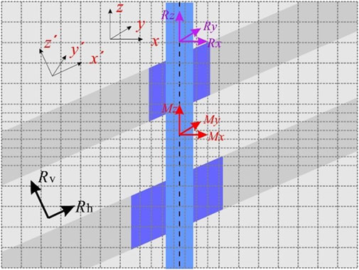
Figure 2. A three-dimensional formation model for EM LWD modeling.

It should be noted that formation conductivity is usually expressed in the formation coordinate system. In EM LWD modeling, it is necessary to rotate the formation coordinate system to the tool coordinate system as expressed in Equation 9:

${\sigma }_t={{\mathbf{R}}^{-1}\sigma }_f\mathbf{R}(9)$

where, σ_t and σ_f are the conductivity matrices in the tool coordinate system and the formation coordinate system, respectively. R is the rotation matrix, which is shown in Equation 10.

$\mathrm{R}=\left[\begin{array}{ccc}\mathit{cos}\theta \mathit{cos}\phi \mathit{cos}\gamma -\mathit{sin}\phi \mathit{sin}\gamma & -\mathit{cos}\theta \mathit{cos}\phi \mathit{sin}\gamma -\mathit{sin}\phi \mathit{cos}\gamma & \mathit{sin}\theta \mathit{cos}\phi \\ \mathit{cos}\theta \mathit{sin}\phi \mathit{cos}\gamma +\mathit{cos}\phi \mathit{sin}\gamma & -\mathit{cos}\theta \mathit{sin}\phi \mathit{sin}\gamma +\mathit{cos}\phi \mathit{cos}\gamma & \mathit{sin}\theta \mathit{sin}\phi \\ -\mathit{sin}\theta \mathit{cos}\gamma & \mathit{sin}\theta \mathit{sin}\gamma & \mathit{cos}\theta \end{array}\right](10)$

where $\theta ,\phi$ and $\gamma$ are the three Euler angles.

3.3 Finite difference scheme

To apply the finite difference method, the electric field wave equation is first expanded into a scalar equation:

$\begin{array}{c}\left(\frac{{\mathit{\partial }}^{\mathbf{2}}{\mathit{E}}_{\mathit{y}}^{\mathit{s}}}{\mathit{\partial }\mathit{x}\mathit{\partial }\mathit{y}}+\frac{{\mathit{\partial }}^{\mathbf{2}}{\mathit{E}}_{\mathit{z}}^{\mathit{s}}}{\mathit{\partial }\mathit{x}\mathit{\partial }\mathit{z}}-\frac{{\mathit{\partial }}^{\mathbf{2}}{\mathit{E}}_{\mathit{x}}^{\mathit{s}}}{\mathit{\partial }{\mathit{y}}^{\mathbf{2}}}-\frac{{\mathit{\partial }}^{\mathbf{2}}{\mathit{E}}_{\mathit{x}}^{\mathit{s}}}{\mathit{\partial }{\mathit{z}}^{\mathbf{2}}}\right)-\mathbf{i}\mathit{\omega }{\mathit{\mu }}_{\mathbf{0}}\left({\mathit{\sigma }}_{\mathit{x}\mathit{x}}{\mathit{E}}_{\mathit{x}}^{\mathit{s}}+{\mathit{\sigma }}_{\mathit{x}\mathit{y}}{\mathit{E}}_{\mathit{y}}^{\mathit{s}}+{\mathit{\sigma }}_{\mathit{x}\mathit{z}}{\mathit{E}}_{\mathit{z}}^{\mathit{s}}\right)\\ =\mathbf{i}\mathit{\omega }{\mathit{\mu }}_{\mathbf{0}}\left[\left({\mathit{\sigma }}_{\mathit{x}\mathit{x}}-{\mathit{\sigma }}_{\mathbf{0}}\right){\mathit{E}}_{\mathit{x}}^{\mathit{i}}+{\mathit{\sigma }}_{\mathit{x}\mathit{y}}{\mathit{E}}_{\mathit{y}}^{\mathit{i}}+{\mathit{\sigma }}_{\mathit{x}\mathit{z}}{\mathit{E}}_{\mathit{z}}^{\mathit{i}}\right]\\ \left(\frac{{\mathit{\partial }}^{\mathbf{2}}{\mathit{E}}_{\mathit{x}}^{\mathit{s}}}{\mathit{\partial }\mathit{x}\mathit{\partial }\mathit{y}}+\frac{{\mathit{\partial }}^{\mathbf{2}}{\mathit{E}}_{\mathit{z}}^{\mathit{s}}}{\mathit{\partial }\mathit{y}\mathit{\partial }\mathit{z}}-\frac{{\mathit{\partial }}^{\mathbf{2}}{\mathit{E}}_{\mathit{y}}^{\mathit{s}}}{\mathit{\partial }{\mathit{x}}^{\mathbf{2}}}-\frac{{\mathit{\partial }}^{\mathbf{2}}{\mathit{E}}_{\mathit{y}}^{\mathit{s}}}{\mathit{\partial }{\mathit{z}}^{\mathbf{2}}}\right)-\mathbf{i}\mathit{\omega }{\mathit{\mu }}_{\mathbf{0}}\left({\mathit{\sigma }}_{\mathit{y}\mathit{x}}{\mathit{E}}_{\mathit{x}}^{\mathit{s}}+{\mathit{\sigma }}_{\mathit{y}\mathit{y}}{\mathit{E}}_{\mathit{y}}^{\mathit{s}}+{\mathit{\sigma }}_{\mathit{y}\mathit{z}}{\mathit{E}}_{\mathit{z}}^{\mathit{s}}\right)\\ =\mathbf{i}\mathit{\omega }{\mathit{\mu }}_{\mathbf{0}}\left[{{\mathit{\sigma }}_{\mathit{y}\mathit{x}}\mathit{E}}_{\mathit{x}}^{\mathit{i}}+\left({\mathit{\sigma }}_{\mathit{y}\mathit{y}}-{\mathit{\sigma }}_{\mathbf{0}}\right){\mathit{E}}_{\mathit{y}}^{\mathit{i}}+{\mathit{\sigma }}_{\mathit{y}\mathit{z}}{\mathit{E}}_{\mathit{z}}^{\mathit{i}}\right]\\ \left(\frac{{\mathit{\partial }}^{\mathbf{2}}{\mathit{E}}_{\mathit{x}}^{\mathit{s}}}{\mathit{\partial }\mathit{x}\mathit{\partial }\mathit{z}}+\frac{{\mathit{\partial }}^{\mathbf{2}}{\mathit{E}}_{\mathit{y}}^{\mathit{s}}}{\mathit{\partial }\mathit{y}\mathit{\partial }\mathit{z}}-\frac{{\mathit{\partial }}^{\mathbf{2}}{\mathit{E}}_{\mathit{z}}^{\mathit{s}}}{\mathit{\partial }{\mathit{x}}^{\mathbf{2}}}-\frac{{\mathit{\partial }}^{\mathbf{2}}{\mathit{E}}_{\mathit{z}}^{\mathit{s}}}{\mathit{\partial }{\mathit{y}}^{\mathbf{2}}}\right)-\mathbf{i}\mathit{\omega }{\mathit{\mu }}_{\mathbf{0}}\left({\mathit{\sigma }}_{\mathit{z}\mathit{x}}{\mathit{E}}_{\mathit{x}}^{\mathit{s}}+{\mathit{\sigma }}_{\mathit{z}\mathit{y}}{\mathit{E}}_{\mathit{y}}^{\mathit{s}}+{\mathit{\sigma }}_{\mathit{z}\mathit{z}}{\mathit{E}}_{\mathit{z}}^{\mathit{s}}\right)\\ =\mathbf{i}\mathit{\omega }{\mathit{\mu }}_{\mathbf{0}}\left[{{\mathit{\sigma }}_{\mathit{z}\mathit{x}}\mathit{E}}_{\mathit{x}}^{\mathit{i}}+{\mathit{\sigma }}_{\mathit{y}\mathit{z}}{\mathit{E}}_{\mathit{y}}^{\mathit{i}}+{\left({\mathit{\sigma }}_{\mathit{z}\mathit{z}}-{\mathit{\sigma }}_{\mathbf{0}}\right)\mathit{E}}_{\mathit{z}}^{\mathit{i}}\right]\end{array}(11)$

It can be observed that the incident and scattered fields of the electric field are separated to the left and right sides of the equation, respectively. The scattered field is the unknown to be solved, while the incident field can be obtained through an analytical solution. Therefore, a linear system of equations can be formed by Equation 11. By using the finite difference method, the differential on the left side of the equation is converted into a difference, thereby obtaining the coefficient matrix for the linear system of equations. For the second-order difference, the coordinates at node (i, j, k) are defined as (x_i, y_j, z_k). The coordinates x_i+1/2, y_j+1/2, and z_k+1/2 correspond to the positions at the midpoints of the cell edges between nodes in the x, y, and z directions, respectively. The distances between two nodes in the x, y, and z directions are Δx_i = x_i+1-x_i,Δy_j = y_j+1-y_j,Δz_k = z_k+1-z_k. The distances from the node centers are Δx_i-1/2 = x_i+1/2-x_i-1/2,Δy_j-1/2 = y_j+1/2-y_j-1/2,Δz_k-1/2 = z_k+1/2-z_k-1/2. The derivation of finite difference schemes is a nontrivial process. Without loss of generality, we take the first term on the left side of Equation 11 as an example. Its finite difference scheme is formulated in Equation 12:

$\begin{array}{c}\frac{{\partial }^2{E}_y^s}{\partial x\partial y}=\frac{\partial }{\partial y}\left(\frac{E_{y\left(i+1,j,k\right)}^s-E_{y\left(i,j,k\right)}^s}{∆x_i}\right)=\frac{1}{∆x_i∆y_{j-\frac{1}{2}}}\\ \times \left[\left(E_{y\left(i+1,j+\frac{1}{2},k\right)}^s-E_{y\left(i,j+\frac{1}{2},k\right)}^s\right)-\left(E_{y\left(i+1,j-\frac{1}{2},k\right)}^s-E_{y\left(i,j-\frac{1}{2},k\right)}^s\right)\right]\end{array}(12)$

The other terms on the left side of the equation can be obtained using the same method. For the terms on the right side, we only need to calculate the incident field at the corresponding nodes using an analytical solution. Another issue in constructing the linear system of equations is the assignment of conductivity values. Since the electric field is located on the edge of a cell and there are four cells surrounding that edge, it is necessary to use the properties of the four cells to equivalently assign the conductivity of the electric field at that location. Here, we use the xx component as an example to derive the equivalent conductivity. Assume that the electric field within any cell is uniform and equal to the electric field at (i+1/2, j, k). For the electric field in the x-direction, the current generated in the x-direction is given by

$\begin{array}{c}{J}_{xx\left(i,j-1,k-1\right)}{S}_{\left(i,j-1,k-1\right)}+J_{xx\left(i,j,k-1\right)}{S}_{\left(i,j,k-1\right)}+J_{xx\left(i,j-1,k\right)}{S}_{\left(i,j-1,k\right)}\\ +J_{xx\left(i,j,k\right)}{S}_{\left(i,j,k\right)}=J_{xx\left(i+\frac{1}{2},j,k\right)}S\end{array}(13)$

where S represents the cross-sectional area. By combining the differential form of Ohm’s law with Equation 13, we obtain the equivalent conductivity as expressed in Equation 14.

$\begin{array}{c}{\sigma }_{xx\left(i+\frac{1}{2},j,k\right)}=\frac{∆z_{k-\frac{1}{2}}\left(∆y_{j-1}{\sigma }_{xx\left(i,j-1,k-1\right)}+∆y_j{\sigma }_{xx\left(i,j,k-1\right)}\right)}{4∆y_{j-\frac{1}{2}}∆z_{k-\frac{1}{2}}}\\ +\frac{∆z_k\left(∆y_{j-1}{\sigma }_{xx\left(i,j-1,k\right)}+∆y_j{\sigma }_{xx\left(i,j,k\right)}\right)}{4∆y_{j-\frac{1}{2}}∆z_{k-\frac{1}{2}}}\end{array}(14)$

The equivalent conductivity for other components can be derived in a similar manner and will not be repeated here.

3.4 Symmetric fields-based half-space modeling method

Typically, due to the complex formation structures and measurement environments, the electromagnetic field distribution generated by the EM LWD tools is quite intricate. However, when the complexity of the formation structure is reduced, and only horizontal layered formations are considered, the electromagnetic field distribution will exhibit certain symmetric or antisymmetric properties. Consider a deviated borehole model within a horizontally layered formation. The top and bottom shoulder beds are modeled as semi-infinite, isotropic formations, with resistivities of 3 Ω·m and 4 Ω·m, respectively. The middle layer is characterized by anisotropic properties, with a horizontal resistivity of 10 Ω·m and a vertical resistivity of 40 Ω·m. The wellbore deviates at an angle of 60° relative to the formation normal, with a radius of 4.25 inches (10.8 cm), and is filled with drilling mud of resistivity 0.1 Ω·m. Mud invasion occurs within the middle layer, extending to a depth of 0.5 m. The invaded zone exhibits a horizontal resistivity of 1 Ω·m and a vertical resistivity of 4 Ω·m. Figure 3 illustrates the cross-sectional view of the electric field in the YOZ plane generated by a magnetic dipole source oriented in the z-direction. It is evident that all components of the electric field are symmetric about the y = 0 plane. Much more numerical simulations indicate that similar results can be observed for magnetic dipole sources oriented in other directions. This symmetry arises from the fact that, although the current model is three-dimensional, it is symmetric about the y = 0 plane. Therefore, the symmetry of the field is an inherent property of the model.

Figure 3

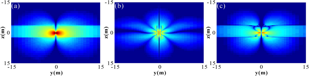
Figure 3. Cross-sectional view of the electric field generated by a magnetic dipole source in the z-direction on YOZ plane: (a) Ex component; (b) Ey component; (c) Ez component.

To further validate the symmetry of the electromagnetic field, a three-dimensional model is established. Specifically, a vertical well is embedded in a homogeneous formation with a resistivity of 10 Ω·m. The borehole has a diameter of 8.5 inches and is filled with mud of resistivity 0.1 Ω·m. The transmitter coil is positioned at the center of the well axis at a relative depth of 0 m, with coordinates (0, 0, 0). A low-resistivity anomaly, characterized by a resistivity of 1 Ω·m and a side length of 2 m, is placed adjacent to the well, with its center located at coordinates (2 m, 0 m, 0 m). Figure 4 presents the cross-sectional distribution of the Ez component on the XOY plane (z = 0.5) generated by different directional dipole sources. The results indicate that the electric field maintains symmetry with respect to the y = 0 plane.

Figure 4

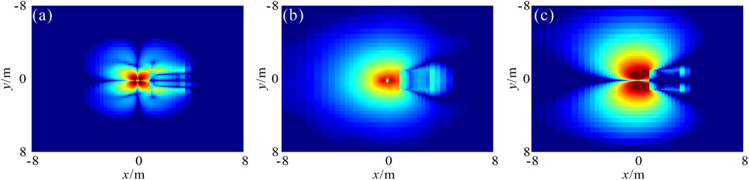
Figure 4. Cross-sectional view of Ez component on XOY plane (z = 0.5m) generated by: (a) x-oriented dipole; (b) y-oriented dipole; (c) z-oriented dipole.

Since the electromagnetic field exhibits symmetrical properties, we can simplify the simulations by computing the field in half of the space. Figure 5a presents a schematic of the electric field nodes on the YOZ plane within a full-space computation domain, while Figure 5b illustrates the corresponding electric field node distribution on the YOZ plane in a half-space computation domain. In this case, we assume the midpoint of the y-axis coordinates $y\left(\frac{Ny+1}{2}\right)$ and $y\left(\frac{Ny+1}{2}+1\right)$ of the symmetry plane. In half-space modeling, a crucial consideration is that by eliminating half of the spatial domain, the boundary conditions of the computational model are consequently altered. Specifically, in the full-space 3D finite difference simulation of EM LWD, PEC boundary conditions are used. However, in the case of half-space modeling, one of the boundaries is transformed into a symmetry plane (i.e., the YOZ plane). On this symmetry plane, the electric field cannot be treated with PEC boundary conditions. In contrast, we can leverage the symmetry of the field to establish new boundary conditions. Assuming the number of grid points in the x, y, and z directions are denoted as Nx, Ny, and Nz, respectively, with each being an odd number. The boundary conditions on the symmetry plane can be set according to Equation 15:

$\left\{\begin{array}{c}{E}_{x\left(i+\frac{1}{2},\frac{Ny+1}{2},k\right)}=sgn\left(M\right)·E_{x\left(i+\frac{1}{2},\frac{Ny+1}{2}+1,k\right)}\\ E_{z\left(i,\frac{Ny+1}{2},k+\frac{1}{2}\right)}=sgn\left(M\right)·E_{z\left(i,\frac{Ny+1}{2}+1,k+\frac{1}{2}\right)}\end{array}\right.(15)$

where sgn (·) is a function of the magnetic dipole moment. For magnetic dipole sources oriented in the x and z directions, sgn (·) equals −1, while for those oriented in the y direction, sgn (·) equals +1. The relative position relationship of the electric field in the equation can be seen in Figure 4B. It should be noted that on the YOZ plane, only electric field components in the x and z directions are present. Therefore, boundary conditions need only be considered for E_x and E_z. Since the computational domain has been reduced to half of its original size, the number of electric field nodes to be solved is similarly halved. Consequently, the computational efficiency can be significantly improved.

Figure 5

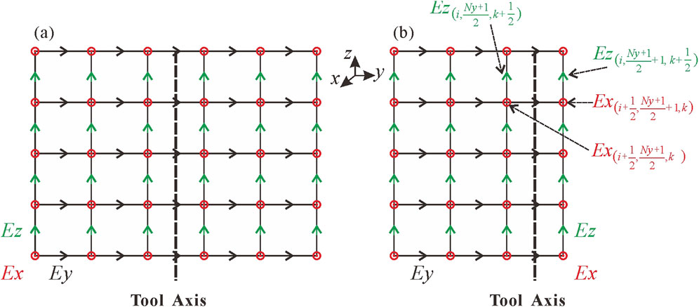
Figure 5. Finite difference grids and electric field nodes. (a) full-space; (b) half-space.

4 Algorithm validation

To validate the accuracy of the algorithm, three models were designed: a homogenous anisotropic formation, a horizontally layered formation, and a mud invasion model. The 3D finite difference simulation results were compared with analytical solutions and results from 3D finite element method. For the homogeneous model, the horizontal and vertical resistivity are set to 5 Ω·m and 20 Ω·m, respectively. The well deviation ranges from 0° to 90°, with the tool operating at a frequency of 100 kHz and a transmitter-receiver spacing of 96 inches. Figure 6a illustrates the variation of the H_xx component of the magnetic field at the receiver as a function of the borehole dip angle. In the figure, the black solid line represents the analytical solution, while the red scattered points indicate the results from the 3D finite difference simulation.

Figure 6

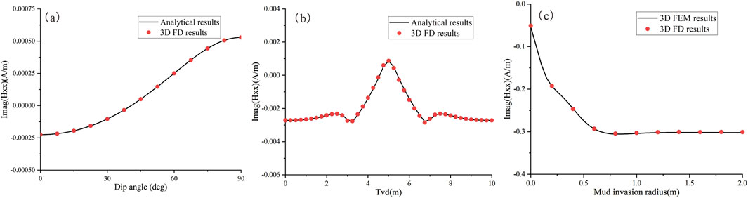
Figure 6. Comparison of 3D finite difference results with the analytical solution and 3D finite element method. (a) Homogeneous Formation Model; (b) Horizontally Layered Formation Model; (c) Mud Invasion Model.

For the horizontally layered formation, the model consists of three layers: the top and bottom shoulder beds are both semi-infinite with a resistivity of 1 Ω·m, and the middle layer is a 2-m thick anisotropic layer with horizontal and vertical resistivities of 10 Ω·m and 40 Ω·m, respectively. The tool frequency is set to 100 kHz, with a transmitter-receiver spacing of 96 inches, and the well deviation angle is 0°. Figure 6b shows the variation of the imaginary part of H_xx component with true vertical depth (Tvd). In the figure, the black solid line represents the analytical solution, while the red scattered points denote the 3D finite difference results. For the mud invasion model, the borehole radius is assumed to be 4.25 inches, filled with mud having a resistivity of 0.5 Ω·m. The resistivities of the invaded zone and the virgin zone are 1 Ω·m and 10 Ω·m, respectively. Figure 6c shows the variation of the imaginary part of H_xx with the invasion radius, where the invasion radius refers to the distance from the boundary of the invaded zone to the wellbore wall. In the figure, the black solid line represents the 3D finite element method results, while the red scattered points denote the 3D finite difference results. It can be observed that in all three tested models, the 3D finite difference simulation results closely match the reference solutions, with relative errors of less than 1%, thereby validating the accuracy of the algorithm.

5 Numerical examples

In this section, we apply the 3D finite difference algorithm to simulate the EM LWD responses and analyze the effects of borehole environment and mud invasion on the responses of different types of EM LWD tools.

5.1 Borehole effects

During the drilling process, the wellbore is typically filled with drilling mud. As a result, the electromagnetic waves generated by EM LWD tools are inevitably influenced by the borehole environment. In this section, we take the Hzz (coaxial component) and Hzx (cross-coupling component) components as examples to analyze the effects of the borehole on the tool response. Consider a three-layer formation model, where the middle resistive layer exhibits a resistivity of 10 Ω·m and a thickness of 3 m. The top and bottom layers are infinitely thick with a resistivity of 1 Ω·m. The formation is penetrated by a vertical borehole. In the first scenario, we ignore the influence of the borehole and consider only the variation in formation resistivity. In the second scenario, we take the borehole effects into account, with a borehole radius of 6 inches and a mud resistivity of 0.2 Ω·m. In this case, we assume a one-transmitter, one-receiver configuration, with an operating frequency of 20 kHz and a transmitter-receiver spacing of 40 inches. Figure 7 illustrates the variation of the imaginary part of the Hzz component with depth in the formation. In Figure 7a, the comparison between the FDFD results and the analytical solutions demonstrates a good agreement, confirming the validity of the 3D finite difference algorithm. Figure 7b compares the response results with and without the presence of a borehole, revealing that the existence of the borehole leads to deviations in the Hzz curve. Since the Hzz component is typically used for measuring apparent resistivity in formations, it is important to appropriately consider the borehole environment during apparent resistivity analysis. Figure 8 illustrates the variation of the Hxz component with depth (in this case, the formation dip angle is 45°, and the other parameters are the same as in Figure 7). Separation of the curves can be observed as the tool approaches the formation boundary. The Hxz component is commonly used for detecting bed boundaries, and significant borehole effects may lead to errors in determining the distance to the boundary. It should be noted that, in most cases, a borehole radius of 4.25 inches is typically used rather than 6 inches. However, in this example, our primary goal is to demonstrate the validity of the method and the overall impact of the borehole on the curves. Therefore, slight variations in borehole size will not affect the conclusions.

Figure 7

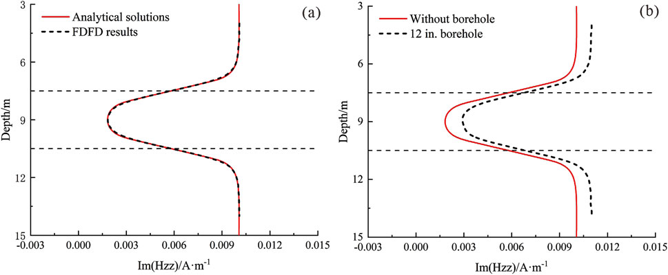
Figure 7. Variation of the imaginary part of the Hzz component with depth. (a) Comparison of FDFD results and analytical solutions in 1D model; (b) Comparison of responses with and without borehole.

Figure 8

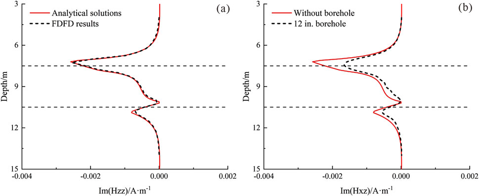
Figure 8. Variation of the imaginary part of the Hxz component with depth. (a) Comparison of FDFD results and analytical solutions in 1D model; (b) Comparison of responses with and without borehole.

When discussing borehole effects, it is essential to consider the influence of mud resistivity. The resistivity of drilling mud can vary significantly; for instance, saline-based muds exhibit very low resistivity, while freshwater and oil-based muds demonstrate much higher resistivity. Consider a homogeneous formation with a resistivity of 10 Ω·m, penetrated by a wellbore with a radius of 4.25 inches. The resistivity of the mud within the wellbore varies from 0.002 to 100 Ω·m. Here, we focus on examining the impact of wellbore mud on the apparent resistivity curve. Figure 9 illustrates the variation in amplitude ratio and phase shift with mud resistivity for electromagnetic logging-while-drilling (LWD) configurations of 2 MHz–28 in and 400 kHz-40 in. As shown in Figure 9a, the amplitude ratio for the 2 MHz-28 in configuration decreases rapidly with increasing mud resistivity, eventually leveling off, indicating the response of a homogeneous medium. In particular, when the mud resistivity is as low as 0.002 Ω·m, the amplitude ratio of the 400 kHz-40 in configuration remains approximately equal to that of a homogeneous formation. In contrast, when the mud resistivity falls below 0.01 Ω·m, the amplitude ratio of the 2 MHz-28 in configuration is significantly affected by the borehole. In Figure 9b, the two curves exhibit singularities in the low-resistivity (high-conductivity) mud region, which may be attributed to the nonlinear phase shift induced by the presence of highly conductive mud. For the 400 kHz-40 in phase difference, the measurement results remain largely unaffected by borehole conditions when the mud resistivity exceeds 0.05 Ω·m. In contrast, the 2 MHz-28 in phase difference remains susceptible to borehole effects unless the mud resistivity exceeds 0.2 Ω·m. Overall, high-frequency phase difference signals exhibit greater sensitivity to low-resistivity mud conditions, whereas low-frequency amplitude ratio signals demonstrate higher robustness against such influences.

Figure 9

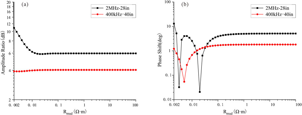
Figure 9. Amplitude ratio and phase shift vary with mud resistivity. (a) Amplitude ratio; (b) Phase shift.

5.2 Mud invasion

In the process of oil and gas well drilling, overbalanced drilling is commonly employed, where the wellbore pressure exceeds the formation pressure, leading to drilling mud invasion into the formation. Considering that logging-while-drilling (LWD) incorporates real-time measurement during the drilling process, the effects of mud invasion are typically neglected. In this paper, we utilize numerical simulation to rigorously investigate the impact of mud invasion on the response characteristics of various logging tools.

First, we consider the impact of mud invasion on apparent resistivity measurements obtained from a conventional EM LWD tool. Two mud invasion models are established as follows: (1) Conductive invasion model: The wellbore radius is 4.25 in, with a mud resistivity of 0.5 Ω·m, a formation resistivity of 10 Ω·m, and an invasion zone resistivity of 1 Ω·m. (2) Resistive invasion model: The wellbore radius is 4.25 in, with a mud resistivity of 1,000 Ω·m, a formation resistivity of 1 Ω·m, and an invasion zone resistivity of 10 Ω·m. Figure 10 illustrates the variation of A28H, P28H, A40L, and P40L with respect to the invasion depth. In this context, A28H and P28H represent the amplitude ratio and phase shift signals from the 2 MHz-28 in configuration, while A40L and P40L represent the amplitude ratio and phase shift signals from the 400 kHz-40 in configuration, respectively. Here, ‘A’ and ‘P’ denote the amplitude ratio and phase shift, respectively, to distinguish the types of signals, while ‘H’ and ‘L’ stand for high frequency and low frequency, respectively, to differentiate between the 2 MHz and 400 kHz signals. It can be observed that conductive invasion increases both the amplitude ratio and phase shift, while resistive invasion results in a decrease in both parameters. The amplitude ratio shows the most significant variation at invasion depths between 0.5 and 1.0 m, while the phase shift exhibits the most pronounced variation between 0 and 0.5 m. When the invasion depth exceeds 1.0 m, neither the amplitude ratio nor phase shift undergoes significant changes with further increases in invasion depth, primarily because the invasion zone extends beyond the detection range of the EM LWD tools.

Figure 10

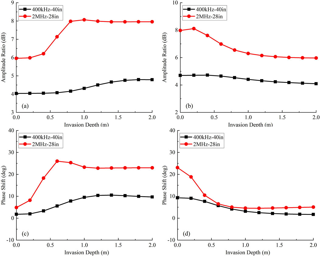
Figure 10. Amplitude ratio and phase shift vary with invasion depth. (a) Amplitude ratio with conductive invasion model; (b) Amplitude ratio with resistive invasion model; (c) Phase shift with conductive invasion model; (d) Phase shift with resistive invasion model.

Figure 11

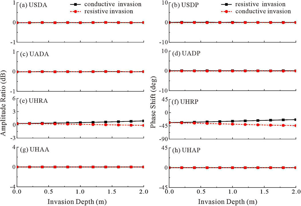
Figure 11. Extra-deep EM LWD responses vary with invasion depth. (a) USDA; (b) USDP; (c) UADA; (d) UADP; (e) UHRA; (f) UHRP; (g) UHAA; (h) UHAP.

Using the same mud invasion models as previously described, we further analyze the variation in the responses of an extra-deep EM LWD tool with different measurement modes as a function of invasion depth, taking the 24 kHz-13 m coil configuration as an example. The numerical simulation results are shown in Figure 11.

The figure demonstrates that mud invasion does not significantly affect the responses of USDA, USDP, UADA, UADP, UHAA, and UHAP. Although mud invasion causes a slight variation in the values of UHRA and UHRP, the effect is minimal, especially when the invasion depth is less than 1 m, where the influence can be considered negligible.

Numerical simulations indicate that the effect of mud invasion on tool responses is strongly dependent on the tool parameters and the type of invasion. For high-frequency, short-spacing signals, mud invasion leads to a deviation of the apparent resistivity from the true formation resistivity. In contrast, for low-frequency, long-spacing signals, the impact of mud invasion is minimal and can generally be disregarded in well logging analysis.

5.3 Resistivity anomaly near the borehole

To further illustrate the applicability of the proposed method, we developed the model presented in Figure 12 to investigate the effect of a resistivity anomalous body adjacent to the borehole on EM LWD responses. In this model, a homogeneous sandstone formation with a resistivity of 10 Ω·m is assumed, incorporating an infinitely long, low-resistivity shale inclusion with a cross-sectional dimension of 2 m × 2 m. A horizontal well traverses beneath the shale, with the borehole positioned at a distance D2A of 1 m from the lower boundary of the shale.

Figure 12

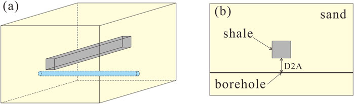
Figure 12. Model of the anomalous body adjacent to the borehole. (a) Three-dimensional model; (b) Two-dimensional cross-sectional view.

Figure 13 illustrates the tool responses obtained from EM LWD, where GA96L and GA96M denote the amplitude ratio signals at 96 in-100 kHz and 96 in-400 kHz, respectively, while GP96L and GP96M represent the phase shift signals at 96 in-100 kHz and 96 in-400 kHz, respectively. It is well established that when the tool operates in a homogeneous formation, geosignals are equal to zero. The detection capability of the tool is typically defined by threshold values of 0.25 dB for the amplitude ratio and 1.5° for the phase shift. As shown in Figure 13a, when adopting 0.25 dB as the threshold, GA96L can detect the presence of the anomalous body at a distance of 2.5 m from its left boundary, whereas GA96M can only detect it within 1.5 m of the left boundary. This observation indicates that lower-frequency signals exhibit greater detection depth. In Figure 13b, due to the relatively small magnitude of the phase shift signal, GP96L fails to detect the anomalous body when using 1.5° as the threshold, while GP96M is capable of detecting it only when the distance to the left boundary is reduced to 0.5 m. These results demonstrate that the amplitude ratio signal provides superior detection capability compared to the phase shift signal.

Figure 13

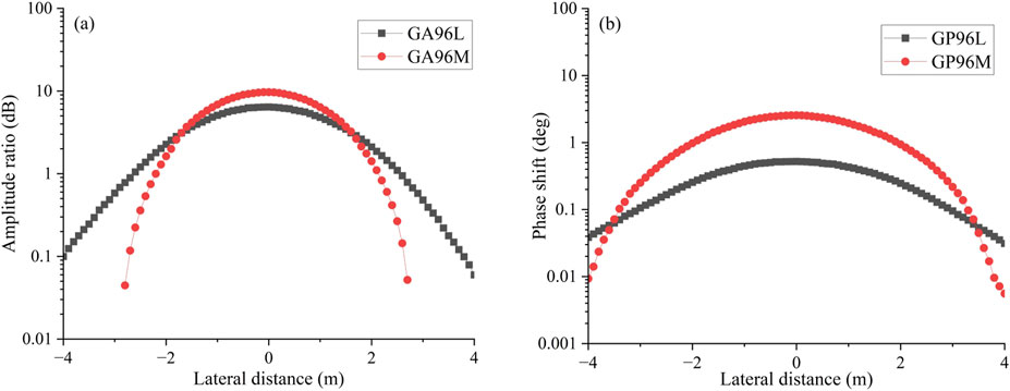
Figure 13. EM LWD geosignals responses: (a) Amplitude ratio; (b) Phase shift.

6 Discussion

Three-dimensional (3D) numerical modeling is the most robust approach for simulating well-logging responses in subsurface formations (Weiss and Newman, 2002; Ma et al., 2014), as these responses are inherently controlled by the synergistic effects of multiple geological factors, including lithological heterogeneity, borehole geometry, and fluid saturation dynamics (Grayver and Bürg, 2014; Kang et al., 2023). However, the substantial memory requirements and computational complexity of 3D numerical modeling significantly constrain its practical application, particularly in data processing workflows where it fails to meet the efficiency demands of interpretation engineers (Zhou et al., 2016). To mitigate these limitations, researchers have developed simplified approaches tailored to specific logging instruments and methodologies. Among these, the sliding window method is the most widely adopted, as it reduces computational costs by incrementally approximating complex 3D models through sequential 2D and 1D representations (Wang et al., 2018). This dimensionality reduction approach is highly effective in improving computational efficiency (Abubakar et al., 2008; Auken and Christiansen, 2004; Lovell and Chew, 1987). However, it remains a simplification method that inherently involves neglecting certain factors, leading to inherent limitations. For instance, when the simultaneous effects of mud invasion and borehole inclination must be considered, a 3D model cannot be adequately reduced to a 2D model.

The fundamental principle of our computational simplification is based on the symmetry of the electromagnetic field. Through theoretical analysis and numerical experiments, we rigorously demonstrate that the electromagnetic field generated in a symmetric formation model also exhibits symmetry. Leveraging this property, we reduce computational complexity by solving for the field in only half of the domain, while the other half is reconstructed using symmetry. The accuracy of the proposed method is further validated through numerical simulations. Moreover, several case studies are presented to illustrate the applicability of the simplified algorithm under various conditions. With the increasing application of extra-deep EM LWD tools, the demand for 3D simulations is expected to grow rapidly. The method proposed in this study holds significant potential for broader applications in this context.

As with all simplification algorithms, the method presented in this study has its limitations. Specifically, it requires that the model being simulated exhibit symmetry. In other words, this method is not universally applicable to all 3D problems. Nonetheless, it is crucial to highlight the advantages of this method and its potential future applications: (a) Our method improves upon traditional 3D algorithms, making it highly cost-effective for researchers or institutions already utilizing 3D simulation programs. (b) When analyzing the impact of individual factors, such as borehole mud, instrument eccentricity, or mud invasion, this algorithm offers a significant advantage by reducing computation time compared to conventional 3D methods. (c) Although the algorithm requires symmetry in the model, it can still serve as an approximate solution for asymmetric models, providing a near solution at a substantially lower computational cost.

7 Conclusion

In this paper, we propose a three-dimensional finite-difference frequency-domain method for electromagnetic (EM) modeling, specifically designed for symmetric geological models. The method is applied to simulate EM Logging-While-Drilling (LWD) tool responses and analyze key influencing factors. Numerical simulations demonstrate that the proposed approach achieves high accuracy in modeling EM LWD responses while significantly reducing computational costs. A detailed analysis of borehole effects reveals that the influence of the borehole environment on apparent resistivity curves is primarily governed by mud resistivity and tool parameters. Generally, tools operating at higher frequencies and with shorter transmitter-receiver (TR) spacings are more susceptible to borehole effects. However, when the mud resistivity exceeds a certain threshold- 0.2 Ω·m in the examples presented in this study—the impact of the borehole can be considered negligible. The effect of mud invasion on logging responses is found to be highly dependent on tool parameters. Specifically, tools operating at higher frequencies and with shorter transmitter-receiver (TR) spacings exhibit greater sensitivity to invasion-induced resistivity contrasts. Conversely, extra-deep EM LWD tools, which typically operate at lower frequencies and employ longer TR spacings, show minimal sensitivity to invasion effects. Given that the invasion depth during logging-while-drilling is generally shallow, the impact of mud invasion on extra-deep EM LWD measurements can be considered negligible in most practical scenarios.

It is important to note that the method proposed in this study is fundamentally a simplified simulation approach tailored for symmetric models. While the current implementation is based on a 3D finite-difference formulation in Cartesian coordinates, the underlying methodology can be extended to cylindrical coordinates, broadening its applicability to a wider range of wellbore and formation geometries. Future research will focus on extending this approach to more complex anisotropic formations and integrating it with inversion algorithms to improve subsurface characterization in challenging geological environments.

Data availability statement

The original contributions presented in the study are included in the article/supplementary material, further inquiries can be directed to the corresponding author.

Author contributions

FL: Funding acquisition, Methodology, Writing – original draft. ZW: Funding acquisition, Investigation, Methodology, Writing – original draft, Writing – review and editing. WN: Funding acquisition, Investigation, Writing – review and editing. XL (4th author): Methodology, Writing – review and editing. XL (5th author): Methodology, Writing – review and editing. HX: Validation, Writing – review and editing. YZ: Validation, Writing – review and editing.

Funding

The author(s) declare that financial support was received for the research and/or publication of this article. We are indebted to the financial support from the National Key R&D Program of China (2019YFA0708301), National Natural Science Foundation of China (42304140), Natural Science Foundation of China (No.U24B6001), and Natural Science Foundation of Sichuan, China (2023NSFSC0771).

Conflict of interest

Authors FL, WN, and XL (4th author) were employed by Sinopec Key Laboratory of Well Logging and Sinopec Research Institute of Petroleum Engineering Co., Ltd.

The remaining authors declare that the research was conducted in the absence of any commercial or financial relationships that could be construed as a potential conflict of interest.

Generative AI statement

The author(s) declare that no Generative AI was used in the creation of this manuscript.

Publisher’s note

All claims expressed in this article are solely those of the authors and do not necessarily represent those of their affiliated organizations, or those of the publisher, the editors and the reviewers. Any product that may be evaluated in this article, or claim that may be made by its manufacturer, is not guaranteed or endorsed by the publisher.

References

Abubakar, A., Habashy, T. M., Druskin, V. L., Knizhnerman, L., and Alumbaugh, D. (2008). 2.5D forward and inverse modeling for interpreting low-frequency electromagnetic measurements. Geophysics 73 (4), F165–F177. doi:10.1190/1.2937466

CrossRef Full Text | Google Scholar

Auken, E., and Christiansen, A. V. (2004). Layered and laterally constrained 2D inversion of resistivity data. Geophysics 69 (3), 752–761. doi:10.1190/1.1759461

CrossRef Full Text | Google Scholar

Bazara, M., Abdelwahid, D. K., and Popov, T. (2016). “Ultra-deep directional resistivity measurements and the way of revealing formation tops ahead of time,” in Abu dhabi international petroleum exhibition and conference.

Google Scholar

Bittar, M. (2000). Electromagnetic wave resistivity tool having a tilted antenna for determining the horizontal and vertical resistivities and relative dip angle in anisotropic earth formations. U.S. Pat. Appl. no. 6 (163)–155.

Google Scholar

Bittar, M., Klein, J., Beste, R., Hu, G., Wu, M., Pitcher, J., et al. (2009). A new azimuthal deep-reading resistivity tool for geosteering and advanced formation evaluation. SPE Reserv. Eval. and Eng. 12 (02), 270–279. doi:10.2118/109971-pa

CrossRef Full Text | Google Scholar

Bittar, M., Rodney, P., Mack, S., and Bartel, R. (1993). A multiple-depth-of-investigation electromagnetic wave resistivity sensor: theory, experiment, and field test results. SPE Form. Eval. 8 (03), 171–176. doi:10.2118/22705-pa

CrossRef Full Text | Google Scholar

Chen, Y., Omeragic, D., Druskin, V., Kuo, C., Habashy, T., Abubakar, A., et al. (2011). “2.5D FD modeling of EM directional propagation tools in high-angle and horizontal wells,” in 81th annual international meeting, SEG, 422–426.

Google Scholar

Clegg, N., Parker, T., Djefel, B., Monteilhet, L., and Marchant, D. (2019). “The final piece of the puzzle: 3-D inversion of ultra-deep azimuthal resistivity lwd data,” in SPWLA 60th annual logging symposium. D043S010R003.

Google Scholar

Clegg, N., Sinha, S., Rodriguez, K. R., Walmsely, A., Sviland-Østre, S., Lien, T., et al. (2022). “Ultra-deep 3D electromagnetic inversion for anisotropy, a guide to understanding complex fluid boundaries in a turbidite reservoir,” in SPWLA 63rd annual logging symposium.

Google Scholar

Davydycheva, S., Druskin, V., and Habashy, T. (2003). An efficient finite-difference scheme for electromagnetic logging in 3D anisotropic inhomogeneous media. Geophysics 68 (5), 1525–1536. doi:10.1190/1.1620626

CrossRef Full Text | Google Scholar

Davydycheva, S., Zhou, M., and Liu, R. (2014). “Triaxial induction tool response in 1D layered biaxial anisotropic formation,” in SEG annual meeting.

Google Scholar

Fan, Y., Hu, X., Deng, S., Yuan, X., and Li, H. (2019). Logging while drilling electromagnetic wave responses in inclined bedding formation. Petroleum Explor. Dev. 46 (4), 711–719. doi:10.1016/S1876-3804(19)60228-4

CrossRef Full Text | Google Scholar

Gao, J., Ke, S., Wei, B., and Tan, M. (2010). Introduction to numerical simulation of electrical logging and its development trend. Well Logging Technol. 34 (01), 1–5. doi:10.16489/j.issn.1004-1338.2010.01.002

CrossRef Full Text | Google Scholar

Grayver, A. V., and Bürg, M. (2014). Robust and scalable 3-D geo-electromagnetic modelling approach using the finite element method. Geophys. J. Int. 198 (1), 110–125. doi:10.1093/gji/ggu119

CrossRef Full Text | Google Scholar

Hong, D., Huang, W., and Liu, Q. (2016). Radiation of arbitrary magnetic dipoles in a cylindrically layered anisotropic medium for well-logging applications. IEEE Trans. Geoscience Remote Sens. 54 (11), 6362–6370. doi:10.1109/TGRS.2016.2582535

CrossRef Full Text | Google Scholar

Hue, Y.-K., Teixeira, F., Martin, L., and Bittar, M. (2005). Three-dimensional simulation of eccentric LWD tool response in boreholes through dipping formations. IEEE Trans. Geoscience Remote Sens. 43 (2), 257–268. doi:10.1109/TGRS.2004.841354

CrossRef Full Text | Google Scholar

Jaysaval, P., Shantsev, D. V., de la Kethulle de Ryhove, S., and Bratteland, T. (2016). Fully anisotropic 3-D EM modelling on a Lebedev grid with a multigrid pre-conditioner. Geophys. J. Int. 207 (3), 1554–1572. doi:10.1093/gji/ggw352

CrossRef Full Text | Google Scholar

Kang, Z., Qin, H., Zhang, Y., Hou, B. B., Hao, X. L., and Chen, G. (2023). Coil optimization of ultra-deep azimuthal electromagnetic resistivity logging while drilling tool based on numerical simulation. J. Petroleum Explor. Prod. Technol. 13 (3), 787–801. doi:10.1007/s13202-022-01575-1

CrossRef Full Text | Google Scholar

Lee, H., and Teixeira, F. (2010). Locally-conformal FDTD for anisotropic conductive interfaces. IEEE Trans. Antennas Propag. 58 (11), 3658–3665. doi:10.1109/TAP.2010.2071362

CrossRef Full Text | Google Scholar

Li, H., and Wang, H. (2016). Investigation of eccentricity effects and depth of investigation of azimuthal resistivity LWD tools using 3D finite difference method. J. Petroleum Sci. Eng. 143, 211–225. doi:10.1016/j.petrol.2016.02.032

CrossRef Full Text | Google Scholar

Li, H., Wang, H., Wang, L., and Zhou, X. (2020a). A modified Boltzmann Annealing Differential Evolution algorithm for inversion of directional resistivity logging-while-drilling measurements. J. Petroleum Sci. Eng. 188, 106916. doi:10.1016/j.petrol.2020.106916

CrossRef Full Text | Google Scholar

Li, K., Gao, J., and Zhao, X. (2020). Tool design of look-ahead electromagnetic resistivity LWD for boundary identification in anisotropic formation. J. Petroleum Sci. Eng. 184, 106537. doi:10.1016/j.petrol.2019.106537

CrossRef Full Text | Google Scholar

Li, Y., Sun, X., Wang, M., and Li, R. (2020b). Numerical simulation and analysis of multicomponent induction logging response in anisotropic formation. IEEE Access 8, 149345–149361. doi:10.1109/ACCESS.2020.3015722

CrossRef Full Text | Google Scholar

Liu, N., Wang, Z., and Liu, C. (2015). The simulations of formation resistivity imaging by applying directional resistivity tool with a joint-coil antenna while drilling. Prog. Geophys. (in Chinese) 30 (6), 2897–2905. doi:10.6038/pg20150659

CrossRef Full Text | Google Scholar

Lovell, J. R., and Chew, W. C. (1987). Response of a point source in a multicylindrcally layered medium. IEEE Transactions on Geoscience and Remote Sensing GE- 25 (6), 850–858. doi:10.1109/TGRS.1987.289757

CrossRef Full Text | Google Scholar

Ma, J., Nie, Z., and Sun, X. (2014). Efficient modeling of large-scale electromagnetic well-logging problems using an improved nonconformal FEM-DDM. IEEE Transactions on Geoscience and Remote Sensing 52 (3), 1825–1833. doi:10.1109/tgrs.2013.2255298

CrossRef Full Text | Google Scholar

Noh, K., Pardo, D., and Torres-Verdín, C. (2022). 2.5-D Deep learning inversion of LWD and deep-sensing EM measurements across formations with dipping faults. IEEE Geoscience and Remote Sensing Letters 19, 1–5. doi:10.1109/LGRS.2021.3128965

CrossRef Full Text | Google Scholar

Pardo, D., and Torres-Verdín, C. (2015). Fast 1D inversion of logging-while-drilling resistivity measurements for improved estimation of formation resistivity in high-angle and horizontal wells. Geophysics 80 (2), E111–E124. doi:10.1190/geo2014-0211.1

CrossRef Full Text | Google Scholar

Qin, Z., Pan, H., Wu, A., Yang, H., Hu, T., Hou, M., et al. (2017). Application of conventional propagation resistivity logging for formation boundary identification in geosteering. Journal of Geophysics and Engineering 14 (5), 1233–1241. doi:10.1088/1742-2140/aa80a0

CrossRef Full Text | Google Scholar

Qin, Z., Tang, B., Wu, D., Luo, S. C., Ma, X. G., Huang, K., et al. (2021). A qualitative characteristic scheme and a fast distance prediction method of multi-probe azimuthal gamma-ray logging in geosteering. Journal of Petroleum Science and Engineering 199, 108244–1-10. doi:10.1016/j.petrol.2020.108244

CrossRef Full Text | Google Scholar

Seydoux, J., Legendre, E., Mirto, E., Dupuis, C., Denichou, J.-M., Bennett, N., et al. (2014). “Full 3D deep directional resistivity measurements optimize well placement and provide reservoir-scale imaging while drilling,” in SPWLA 55th annual logging symposium (Abu Dhabi, UAE: SPWLA-2014-LLLL).

Google Scholar

Sun, Q., and Hu, Y. (2022). Fast geometric multigrid preconditioned finite-difference frequency-domain method for borehole electromagnetic sensing. IEEE Geoscience and Remote Sensing Letters 19, 1–4. doi:10.1109/LGRS.2021.3053590

CrossRef Full Text | Google Scholar

Sun, Q., Ren, Q., Zhan, Q., and Liu, Q. (2017). 3-D Domain decomposition based hybrid finite-difference time-domain/finite-element time-domain method with nonconformal meshes. IEEE Transactions on Microwave Theory and Techniques 65 (10), 3682–3688. doi:10.1109/TMTT.2017.2686386

CrossRef Full Text | Google Scholar

Tian, Y., Zhu, J., Die, Y., Liu, L., Yue, C., Wang, X., et al. (2023). Boundary detection capability and influencing factors of electromagnetic resistivity while using drilling tools in a horizontal well. Frontiers in Earth Science 10. doi:10.3389/feart.2022.1042353

CrossRef Full Text | Google Scholar

Wang, H., Wang, H., Yang, S., and Yin, C. (2020a). Efficient finite-volume simulation of the LWD orthogonal azimuth electromagnetic response in a three-dimensional anisotropic formation using potentials on cylindrical meshes. Applied Geophysics 17 (2), 192–207. doi:10.1007/s11770-020-0818-6

CrossRef Full Text | Google Scholar

Wang, L., Fan, Y., Yuan, C., Wu, Z., Deng, S., and Zhao, W. (2018). Selection criteria and feasibility of the inversion model for azimuthal electromagnetic logging while drilling (LWD). Petroleum Exploration and Development 45 (5), 974–982. doi:10.1016/S1876-3804(18)30101-0

CrossRef Full Text | Google Scholar

Wang, L., Wu, Z., Fan, Y., and Huo, L. (2020b). Fast anisotropic resistivities inversion of logging-while-drilling resistivity measurements in high-angle and horizontal wells. Applied Geophysics 17 (3), 390–400. doi:10.1007/s11770-020-0830-x

CrossRef Full Text | Google Scholar

Wang, T., and Fang, S. (2001). 3-D electromagnetic anisotropy modeling using finite differences. Geophysics 66 (5), 1386–1398. doi:10.1190/1.1486779

CrossRef Full Text | Google Scholar

Wang, Y., Wang, H., Kang, Z., and Yin, C. (2023). Efficient computation of nonlinear Born approximation of the LWD ultra-deep look ahead resistivity measurement using coupled potentials 3D finite-volume method and differential operator expansion. Chinese Journal of Geophysics (in Chinese)VL - 66 (7), 3102–3114. doi:10.6038/cjg2022Q0650

CrossRef Full Text | Google Scholar

Wei, K., Qin, Z., Wang, C., Zhang, Z., Su, K., Wang, G., et al. (2024). Response characteristics and novel understandings of dual induction logging of horizontal wells in fractured reservoirs. Journal of Applied Geophysics 225, 105393, 1–10. doi:10.1016/j.jappgeo.2024.105393

CrossRef Full Text | Google Scholar

Weiss, C. J., and Newman, G. A. (2002). Electromagnetic induction in a fully 3-D anisotropic earth. Geophysics 67 (4), 1104–1114. doi:10.1190/1.1500371

CrossRef Full Text | Google Scholar

Wu, B., Yang, Z., Guo, T., and Yuan, X. (2022a). Response characteristics of logging while drilling system with multi-scale azimuthal electromagnetic waves. Petroleum Drilling Techniques 50 (6), 7–13. doi:10.11911/syztjs.2022107

CrossRef Full Text | Google Scholar

Wu, H.-H., Golla, C., Parker, T., Clegg, N., and Monteilhet, L. (2018). “A new ultra-deep azimuthal electromagnetic LWD sensor for reservoir insight,” in SPWLA 59th annual logging symposium.

Google Scholar

Wu, Z., Deng, S., He, X., Zhang, R., Fan, Y., Yuan, X., et al. (2020a). Numerical simulation and dimension reduction analysis of electromagnetic logging while drilling of horizontal wells in complex structures. Petroleum Science 17 (3), 645–657. doi:10.1007/s12182-020-00444-y

CrossRef Full Text | Google Scholar

Wu, Z., Fan, Y., Wang, J., Zhang, R., and Liu, Q. (2020b). Application of 2.5-D Finite difference method in Logging-While-Drilling electromagnetic measurements for complex scenarios. IEEE Geoscience and Remote Sensing Letters 17 (4), 577–581. doi:10.1109/LGRS.2019.2926740

CrossRef Full Text | Google Scholar

Wu, Z., Li, H., Han, Y., Zhang, R., Zhao, J., and Lai, Q. (2022b). Effects of formation structure on directional electromagnetic logging while drilling measurements. Journal of Petroleum Science and Engineering 211, 110118. doi:10.1016/j.petrol.2022.110118

CrossRef Full Text | Google Scholar

Xu, L., Zhang, R., Sun, S., Sun, J., and Shi, J. (2023). Modified levenberg–marquardt inversion for high-resolution resistivity distribution reconstruction of multilayered formation. IEEE Transactions on Instrumentation and Measurement 72, 1–10. doi:10.1109/TIM.2022.3224519

PubMed Abstract | CrossRef Full Text | Google Scholar

Yuan, N., Liu, R., and Nie, X. (2011). “Electromagnetic field of arbitrarily oriented coil antennas in complicated underground environment,” in 2011 IEEE international symposium on antennas and propagation (APSURSI), 1658–1661.

Google Scholar

Yue, X., Liu, T., Li, G., Nie, Z., Ma, M., and Sun, X. (2022). An analytically fast forward method of LWD azimuthal electromagnetic measurement and its geo-steering application. Chinese Journal of Geophysics (in Chinese)VL - 65 (5), 1909–1920. doi:10.6038/cjg2022P0233

CrossRef Full Text | Google Scholar

Zeng, S., Chen, F., Li, D., Chen, J., and Chen, J. (2018). A novel 2.5D finite difference scheme for simulations of resistivity logging in anisotropic media. Journal of Applied Geophysics 150, 144–152. doi:10.1016/j.jappgeo.2018.01.021

CrossRef Full Text | Google Scholar

Zhang, P., Deng, S., Hu, X., Wang, L., Wang, Z., Yuan, X., et al. (2021). Detection performance and sensitivity of logging-while-drilling extra-deep azimuthal resistivity measurement. Chinese Journal of Geophysics (in Chinese)VL - 64 (6), 2210–2219. doi:10.6038/cjg2021O0087

CrossRef Full Text | Google Scholar

Zhang, R., Wu, Z., Sun, Q., Zhuang, M., Cai, Q., Wang, D., et al. (2020). Memory-Efficient 3-D LWD solver with the flipped total field/scattered field-based DGFD method. IEEE Geoscience and Remote Sensing Letters 17 (9), 1498–1502. doi:10.1109/LGRS.2019.2950659

CrossRef Full Text | Google Scholar

Zhou, J., Li, H., Rabinovich, M., and D'Arcy, B. (2016). “Interpretation of azimuthal propagation resistivity measurements: modeling, inversion, application and discussion,” in SPWLA 57th annual logging symposium (Reykjavik, Iceland: SPWLA-2016-HHHH).

Google Scholar