Simultaneous seismic inversion for fluid indicator and brittleness index in the gas-bearing shale reservoir

Accurate estimation of brittleness index, characterizing the brittleness level of rocks, and reservoir fluid identification are crucial for the characterization and development of shale gas reservoirs. However, conventional seismic methods for the sweet spot parameters failed to realize the simultaneous inversion of fluid indicator and brittleness index, challenging exploration of the favorable fracturing areas for shale gas production. For this issue, we concentrate on the simultaneous seismic inversion method of fluid indicator and brittleness index. First, we have derived a novel PP-wave reflection coefficient equation incorporating the above sweet spot parameters, allowing the direct estimation of reservoir brittleness and fluid properties. Two groups of classical layered medium models are introduced to justify the high accuracy of the novel equation within the incidence angle of 40°. Then, to effectively decouple these parameters from the pre-stack seismic data, anisotropic total variation based on L_P norm sparse constraint (ATpV) seismic inversion method is introduced to obtain accurate inversion results, extracting sparser priori information through the strong sparsity of the L_P norm. Numerical model examples demonstrate the high stability and robustness of the proposed simultaneous inversion method. Ultimately, we applied it to field seismic data from a gas-bearing shale reservoir in the Sichuan Basin, China. A comprehensive analysis of the three-dimensional (3D) inversion results with logging, geological structure, and micro-seismic events detected from horizontal fracturing wells has validated the rationality of the method.

1 Introduction

Shale rock, bearing enormous resource potential for shale gas, is widely distributed in the world. However, most shale gas reservoirs process low permeability and porosity, resulting in the requirement for fracturing to facilitate reservoir volumetric modification and increase natural gas production capacity (Buyanov, 2011; Jia et al., 2012; Wen et al., 2024). Therefore, evaluating the gas content of shale gas reservoirs and the brittleness characteristics of reservoir rocks with high precision and then searching for favorable “sweet spot” zones can significantly reduce the exploration cost of shale gas, promote production, and obtain higher economic benefits.

Fluid identification, which began in the 1970s, refers to using seismic data to identify and characterize fluid-bearing reservoirs, facilitating the direct detection of hydrocarbons. Smith and Gidlow (1987) were the first to propose the concept of fluid factors. They introduced a weighted superposition method based on AVO (Amplitude Variation with Offset) analysis. This method can leverage the relative changes in P-wave and S-wave velocities to distinguish hydrocarbon anomalies within a reservoir. Goodway et al. (1997) proposed a fluid identification method based on LMR (λ-μ-ρ) technology, which analyzes the pore fluid characteristics based on the tensile properties of the rock itself. Hedlin (2000) proposed a pore space modulus sensitive to lithology based on studies such as Murphy et al. (1993). Based on the Biot-Gassmann equation, Russell et al. (2003) derived a fluid property (ρf) that is more sensitive to reservoir fluids and more applicable for fluid identification than LMR techniques. Quakenbush et al. (2006) combined Poisson’s ratio and density to develop the concept of Poisson’s impedance (product of Poisson’s ratio and density), which can distinguish reservoir fluids more effectively than a single parameter. Ning et al. (2006) summarized and classified the fluid identification indicators and proposed constructing higher-order fluid indicators to satisfy different reservoir prediction tasks according to the needs and conditions. Researchers typically represent fluid indicators as a combination of wave impedance and density parameters. Pre-stack three-parameter seismic inversion allows the extraction of various elastic attribute parameters. By integrating these parameters with fluid identification techniques, reservoir fluid identification can be carried out more effectively.

Accurately estimating the brittleness characteristics of reservoir rocks can provide a basis for assessing reservoir modification potential. It also supports selecting sweet spot areas for development and enhances oil and gas recovery efficiency (Li, 2023). The brittleness index is crucial for characterizing a rock’s fracturing potential. Rocks with a high brittleness index are more accessible to fracture, making shale reservoirs more conducive to natural gas development and production (Mullen, 2010; Jin et al., 2015; Li, 2022). Rickman et al. (2008) statistically analyzed the Barnet Shale and concluded that the brittleness index of the rock is positively correlated with Young’s modulus. Young’s modulus cannot be obtained directly from actual seismic data, and the density term needs to be solved beforehand. However, extracting density is challenging due to its insensitivity to reflection amplitude changes. Therefore, Sharma and Chopra (2015) proposed a new expression for the brittleness index, Eρ (the product of Young’s modulus and density), better highlighting anomalous characteristics in shale reservoirs. Luan et al. (2014) derived an expression for the brittleness index of the ratio of Young’s modulus to Poisson’s ratio based on petrophysics, which can lead to a significant value of brittleness index because the brittleness index has a magnitude scale. The two parameters differ significantly in order of magnitude, which does not make it easy to observe and compare. Later, for comparison, Liu and Sun (2015) normalized the two parameters to evaluate the brittleness of reservoir rocks better. Then, analysis results based on shale petrophysical modeling, Chen et al. (2014) proposed the E/λ (ratio of Young’s modulus to the first Lamé constant) attribute as a new brittleness index, which has better sensitivity to the brittleness of shale and can better indicate favorable reservoirs in gas-bearing shale.

In recent years, seismic inversion using actual pre-stack seismic data to obtain fluid indicators for evaluating the fluid-bearing characteristics of target reservoirs and brittleness indices for quantifying the brittleness characteristics of reservoir rocks have been rapidly developed. Based on Gray’s approximation equation, Chi and Han (2006) proposed a method for direct inversion of Lame parameters using pre-stack seismic AVO inversion. Russell et al. (2011) derived the AVO approximation equation, including fluid term, shear modulus, and density, based on the theory of poroelasticity, realizing a direct inversion of the Gassmann fluid term. Zong et al. (2012c) derived a new approximate equation, which can directly invert the performances of E, $\sigma$, and $\rho$, reducing the error of the brittleness index. Zhang et al. (2014) used the PP- and P-SV waves stacking front joint inversion method to directly invert the brittleness index Eρ for shale gas reservoir evaluation. Yin et al. (2015) added model constraints to the inversion objective function to improve the accuracy of the brittleness index inversion results and solved it using a basis pursuit algorithm. Zhang F. Q. et al. (2017) inverted the brittleness index using a basis pursuit algorithm to obtain more accurate inversion results by deriving the brittleness index into the exact Zoeppritz equation. In order to improve the inversion results by getting over the unreliability of extensive offset seismic data, Sun et al. (2021) proposed a method to invert the predicted brittleness characteristics of shale reservoirs using the extended elastic impedance equation. Ge et al. (2022) derived a new approximate equation for the reflection coefficient by combining scattering theory and Born’s equation, and they used a Bayesian framework to realize the pre-stack seismic AVO inversion, which can well portray the brittleness of the reservoir.

We can find that most current studies only assess the reservoir fluid properties or rock fragility individually, and they are usually indirect inversion methods: first, invert the elasticity parameters and then calculate the required fluid indicator and brittleness index through the petrophysical equations. However, due to the inherent uncertainty of the seismic inverse problem, such as the “pathological solution” and the inevitable cumulative error caused by the indirect method, these will make the inversion results highly multi-solutional, which makes it challenging to meet the needs of fluid identification and rock brittleness characterization in actual shale reservoirs. Therefore, this paper derived a new approximation equation based on the Aki-Richards equation to simultaneously and directly acquire highly reliable and stable fluid identification indicators and brittleness index. Meanwhile, we introduced a sparse inversion algorithm to solve the inversion objective function containing the new approximate equation. The inversion method based on this new equation enables the stable and accurate extraction of fluid indicators and brittleness indices directly from pre-stack seismic data, offering a reliable geophysical method for identifying the “sweet spot” of shale gas reservoirs.

2 Theory and method

2.1 Approximation equation in terms of fluid indicator, brittleness index and density

Due to the highly nonlinear nature of the exact Zoeppritz equation, it is challenging to apply it to practical seismic inversion, and scholars have developed various forms of approximate equations for the reflection coefficients (Shuey, 1985; Fatti and Smith, 1994; Zong et al., 2012a; Zong et al., 2012b; Zong et al., 2012c; Zhang S. et al., 2017; Li et al., 2022). One of the most commonly used approximate equations is the Zoeppritz approximation equation proposed by Aki and Richards (2001):

$R_{PP}^{A\text{ki}}\left(\theta \right)=\frac{1}{2}{\sec }^2\theta \frac{\Delta V_P}{\overline{V_P}}-4\gamma {\sin }^2\theta \frac{\Delta V_S}{\overline{V_S}}+\frac{1}{2}\left(1-4\gamma {\sin }^2\theta \right)\frac{\Delta \rho }{\overline{\rho }}(1)$

where θ is the angle of incidence; $\Delta V_P$, $\Delta V_S$ and $\Delta \rho$ denote the differences of the P-wave velocity $V_P$, S-wave velocity, $V_S$ and density $\rho$ values across the boundary, and:

$\gamma ={\left(\frac{\overline{V_S}}{\overline{V_P}}\right)}^2(2)$

where $\overline{V_P}$ and $\overline{V_S}$ represent the average velocity of the P-wave and S-wave, respectively.

Constructing rational forms of fluid indicators plays a crucial role in reservoir fluid prediction, the most common forms being the Lamé parameters and their combinations with other elastic parameters. Goodway et al. (1997) established a fluid indicator (expressed as the product of the first Lamé constant and the density), which can sensitively characterize the rock feature and is a commonly used elastic parameter for fluid prediction. Therefore, the fluid indicator of the gas-bearing shale reservoir can be expressed as:

$F=\lambda \rho (3)$

Young’s modulus E, among other commonly used brittleness indices, is a standard parameter for characterizing the brittleness of shale reservoir rocks. Ongoing research has shown that while Young’s modulus can reflect the influence of brittle minerals like quartz in shale, it has been observed that the presence of organic matter, fluids, and porosity in gas-bearing shale reservoirs can significantly weaken the sensitivity to brittle shales. Consequently, the effectiveness of Young’s modulus as an indicator of shale reservoir brittleness is limited (Kumar et al., 2012; Pan et al., 2020; Ma et al., 2023). To address this, Chen et al. (2014) proposed a new brittleness index, BI = E/λ. Through rock physics modeling, this index has been shown to effectively capture the content of minerals, including quartz, and the combined effects of organic content, fluids, and porosity in shale reservoirs, making it more effective in characterizing gas-bearing brittle rocks. To facilitate the derivation of the approximate equation that follows, we express BI in terms of Poisson’s ratio alone:

$BI=\frac{E}{\lambda }=\frac{\left(1+\sigma \right)\left(1-2\sigma \right)}{\sigma }(4)$

First, the $V_P$ and $V_S$ are related to the P-wave modulus M and S-wave modulus μ in an isotropic elastic medium as follows:

$V_P=\sqrt{\frac{M}{\rho }},V_S=\sqrt{\frac{\mu }{\rho }}(5)$

According to the chain rule of multivariable calculus, we can obtain the following equations about $\Delta V_P$ and $\Delta V_S$:

$\Delta V_P=\Delta M\frac{\mathrm{\partial }{V}_P}{\mathrm{\partial }M}+\Delta \rho \frac{\mathrm{\partial }{V}_P}{\mathrm{\partial }\rho }=\frac{1}{2}\Delta M\sqrt{\frac{1}{\rho }}{M}^{-\frac{1}{2}}-\frac{1}{2}\Delta \rho \sqrt{M}{\rho }^{-\frac{3}{2}}(6)$

$\Delta V_S=\Delta M\frac{\mathrm{\partial }{V}_S}{\mathrm{\partial }\mu }+\Delta \rho \frac{\mathrm{\partial }{V}_S}{\mathrm{\partial }\rho }=\frac{1}{2}\Delta \mu \sqrt{\frac{1}{\rho }}{\mu }^{-\frac{1}{2}}-\frac{1}{2}\Delta \rho \sqrt{\mu }{\rho }^{-\frac{3}{2}}(7)$

Dividing both sides of Equations 6, 7 by $V_P$ and $V_S$, respectively. We obtain the following equations:

$\frac{\Delta V_P}{V_P}=\frac{1}{2}\left(\frac{\Delta M}{M}-\frac{\Delta \rho }{\rho }\right)(8)$

$\frac{\Delta V_S}{V_S}=\frac{1}{2}\left(\frac{\Delta \mu }{\mu }-\frac{\Delta \rho }{\rho }\right)(9)$

In isotropic media, the M and μ have the following relationship:

$M=E\frac{1-\sigma }{\left(1+\sigma \right)\left(1-2\sigma \right)}(10)$

$\mu =\frac{E}{2\left(1+\sigma \right)}.(11)$

Then, we rewrite the fluid indicator F as follows:

$F=\frac{E\sigma \rho }{\left(1+\sigma \right)\left(1-2\sigma \right)}(12)$

Introduce intermediate variables ${\mathrm{{\rm H}}}_A$, ${\mathrm{{\rm H}}}_B$ and ${\mathrm{{\rm H}}}_C$ such that they are:

${\mathrm{{\rm H}}}_A=\frac{1-2\sigma }{\sigma },{\mathrm{{\rm H}}}_B=1+\sigma ,{\mathrm{{\rm H}}}_C=\frac{1-\sigma }{1-2\sigma }(13)$

Substituting Equation 13 into Equations 4, 10–12, we get the following equations

$F=\frac{E\rho }{{\mathrm{{\rm H}}}_A{\mathrm{{\rm H}}}_B},BI={\mathrm{{\rm H}}}_A{\mathrm{{\rm H}}}_B,M=\frac{E{\mathrm{{\rm H}}}_C}{{\mathrm{{\rm H}}}_B},\mu =\frac{E}{{\mathrm{{\rm H}}}_B}(14)$

Similarly, same as Equations 8, 9, we get the following equations:

$\frac{\Delta F}{\overline{F}}=\frac{\Delta E}{\overline{E}}-\frac{\Delta {\mathrm{{\rm H}}}_A}{{\overline{\mathrm{{\rm H}}}}_A}-\frac{\Delta {\mathrm{{\rm H}}}_B}{{\overline{\mathrm{{\rm H}}}}_B}+\frac{\Delta \rho }{\overline{\rho }},\frac{\Delta BI}{\overline{BI}}=\frac{\Delta {\mathrm{{\rm H}}}_A}{{\overline{\mathrm{{\rm H}}}}_A}+\frac{\Delta {\mathrm{{\rm H}}}_B}{{\overline{\mathrm{{\rm H}}}}_B}(15)$

$\frac{\Delta M}{\overline{M}}=\frac{\Delta E}{\overline{E}}+\frac{\Delta {\mathrm{{\rm H}}}_C}{{\overline{\mathrm{{\rm H}}}}_C}-\frac{\Delta {\mathrm{{\rm H}}}_B}{{\overline{\mathrm{{\rm H}}}}_B},\frac{\Delta \mu }{\overline{\mu }}=\frac{\Delta E}{\overline{E}}-\frac{\Delta {\mathrm{{\rm H}}}_B}{{\overline{\mathrm{{\rm H}}}}_B}(16)$

The term about $\frac{\Delta {\mathrm{{\rm H}}}_A}{{\overline{\mathrm{{\rm H}}}}_A}$ has the following definition:

$\frac{\Delta {\mathrm{{\rm H}}}_A}{{\overline{\mathrm{{\rm H}}}}_A}=\frac{2\left({\sigma }_1-{\sigma }_2\right)}{{\sigma }_1+{\sigma }_2-4{\sigma }_1{\sigma }_2}(17)$

where ${\sigma }_1$ and ${\sigma }_2$ denote the Poisson’s ratios of the upper layer and lower layer, respectively, with the following expressions:

${\sigma }_1=\sigma -\frac{\Delta \sigma }{2},{\sigma }_2=\sigma +\frac{\Delta \sigma }{2}(18)$

Substituting Equation 18 into Equation 17, assuming relatively weak variations in elastic parameters when crossing the elastic interface, the higher order terms about ${\left(\Delta \sigma \right)}^2$ can be approximated as zero neglected, we can obtain as:

$\frac{\Delta {\mathrm{{\rm H}}}_A}{{\overline{\mathrm{{\rm H}}}}_A}=\frac{2\sigma }{4{\sigma }^2-2\sigma +{\left(\Delta \sigma \right)}^2}\frac{\Delta \sigma }{\overline{\sigma }}=\frac{1}{2\sigma -1}\frac{\Delta \sigma }{\overline{\sigma }}(19)$

Similarly, we can get results for the terms about $\frac{\Delta {\mathrm{{\rm H}}}_B}{{\overline{\mathrm{{\rm H}}}}_B}$ and $\frac{\Delta {\mathrm{{\rm H}}}_C}{{\overline{\mathrm{{\rm H}}}}_C}$:

$\frac{\Delta {\mathrm{{\rm H}}}_B}{{\overline{\mathrm{{\rm H}}}}_B}=\frac{\sigma }{\sigma +1}\frac{\Delta \sigma }{\overline{\sigma }}(20)$

$\frac{\Delta {\mathrm{{\rm H}}}_C}{{\overline{\mathrm{{\rm H}}}}_C}=\frac{\sigma }{\left(2\sigma -1\right)\left(\sigma -1\right)}\frac{\Delta \sigma }{\overline{\sigma }}(21)$

Next, substituting Equations 19–21 into Equations 15, 16 yields:

$\frac{\Delta F}{\overline{F}}+\frac{\Delta BI}{\overline{BI}}=\frac{\Delta E}{\overline{E}}+\frac{\Delta \rho }{\overline{\rho }},\frac{\Delta BI}{\overline{BI}}=\frac{3\sigma }{\left(2\sigma -1\right)\left(\sigma +1\right)}\frac{\Delta \sigma }{\overline{\sigma }}(22)$

$\frac{\Delta M}{\overline{M}}=\frac{\Delta E}{\overline{E}}+\frac{-2{\sigma }^3+4{\sigma }^2}{\left(2\sigma -1\right)\left(\sigma -1\right)\left(\sigma +1\right)}\frac{\Delta \sigma }{\overline{\sigma }},\frac{\Delta \mu }{\overline{\mu }}=\frac{\Delta E}{\overline{E}}-\frac{\sigma }{\sigma +1}\frac{\Delta \sigma }{\overline{\sigma }}(23)$

Meanwhile, a Poisson’s ratio relationship subscript exists as:

$\sigma =\frac{1-2\gamma }{2\left(1-\gamma \right)}(24)$

By observing the above equations, we first substitute Equations 8, 9, 23 into Equation 1, and then through Equation 22, we replace the E term and $\sigma$ term in it with the F term and the BI term, and replace $\sigma$ in it with Equation 24. Finally, a new approximate equation that allows to obtain both the fluid indicator and the brittleness index has been established:

$R_{PP}^{FBD}\left(\theta \right)={\mathrm{{\rm K}}}_F\left(\theta \right)\frac{\Delta F}{\overline{F}}+{\mathrm{{\rm K}}}_{BI}\left(\theta \right)\frac{\Delta BI}{\overline{BI}}+{\mathrm{{\rm K}}}_{\rho }\left(\theta \right)\frac{\Delta \rho }{\overline{\rho }}(25)$

with

$\left\{\begin{array}{l}{\mathrm{{\rm K}}}_F\left(\theta \right)=\frac{1}{4}{\sec }^2\theta -2\gamma {\sin }^2\theta \\ {\mathrm{{\rm K}}}_{BI}\left(\theta \right)=\frac{4{\gamma }^2-7\gamma +3}{6{\gamma }^2-8\gamma +3}\left(\frac{1}{2}\gamma {\sec }^2\theta -2\gamma {\sin }^2\theta \right)\\ {\mathrm{{\rm K}}}_{\rho }\left(\theta \right)=\frac{1}{2}\left(1-{\sec }^2\theta +4\gamma {\sin }^2\theta \right)\end{array}\right.(26)$

2.2 Approximate equation accuracy analysis

To verify the accuracy of the newly proposed approximate equation in Equation 25, we tested and analyzed it using the three-layer gas-bearing sandstone and shale model given by Goodway et al. (1997) based on the measured data, and the relevant elastic parameters are shown in Table 1.

Table 1

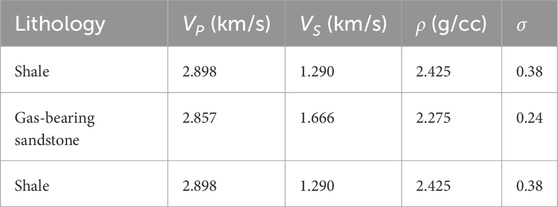
Table 1. The three-layer gas-bearing sandstone and shale model (Goodway et al., 1997).

Based on the model mentioned above, we calculated the reflection coefficients and the residuals between the approximate and exact equations for different interfaces at incidence angles from 0° to 40° using the exact Zoeppritz equation, the Aki-Richard equation, and our proposed equation, respectively.

Figures 1A, 2A show the response curves in the PP-wave reflection coefficients of the three equations at the reflection interfaces of overlying sandstone and underlying shale and the reflection interfaces of overlying shale and underlying gas-bearing sandstone, respectively. Figures 1B, 2B show the variation in the difference between the reflection coefficients calculated using the Aki-Richards equation and our proposed equation, compared to those calculated using the exact Zoeppritz equation, for a range of incidence angles from 0° to 40°. From Figures 1, 2, we can find that the new approximate equation of reflection coefficient and the exact Zoeppritz equation are the same within the range of 40° of incidence angle, and their errors are within the acceptable range, which can be used in the seismic inversion of AVO elastic parameters.

Figure 1

Figure 1. (A) Is the response curve of the PP-wave reflection coefficient of the three equations at the reflection interface of the overlying sandstone and underlying shale; (B) is the error of the new approximation equation and Aki Richard approximation equation compared to the exact Zoeppritz equation.

Figure 2

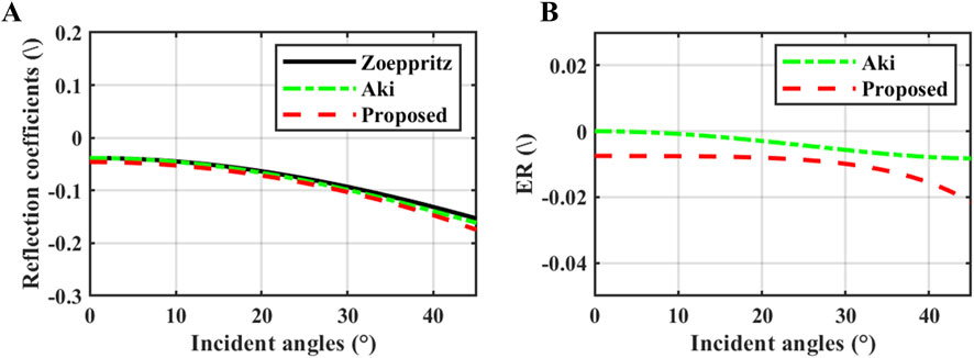
Figure 2. (A) Is the response curve of the PP-wave reflection coefficient of the three equations at the reflection interface of the overlying shale and the underlying gas-bearing sandstone; (B) is the error of the new approximation equation and Aki Richard approximation equation compared to the exact Zoeppritz equation.

2.3 AVO seismic inversion with the sparse constraints of the ATpV regularization

In geophysical problems, a noisy seismic signal can be represented by the reflection coefficient Equation 25 convolution with the seismic wavelet:

$S=w*R_{PP}^{FBD}+\stackrel{\sim }{N}(27)$

Convert the above equation into a matrix multiplication operation:

$\mathit{S}=\mathit{W}\mathit{R}+\stackrel{\sim }{\mathit{N}}(28)$

where $\mathit{S}\in {\mathbb{R}}^{m\times n}$ denotes seismic data and $\mathit{R}\in {\mathbb{R}}^{m\times n}$ denotes the reflection coefficient, $\stackrel{\sim }{\mathit{N}}\in {\mathbb{R}}^{m\times n}$ denotes random noise; m and n are the number of sampling points and traces of seismic data, respectively. W is the wavelet kernels matrix obtained by time-shifting the seismic wavelet Q:

$\mathit{W}={\left[\begin{array}{llll}Q\left(1\right)& 0& \cdots & 0\\ ⋮& Q\left(1\right)& \ddots & ⋮\\ Q\left(i\right)& ⋮& \ddots & 0\\ 0& Q\left(i\right)& ⋮& Q\left(1\right)\\ ⋮& \ddots & \ddots & ⋮\\ 0& \cdots & \ddots & Q\left(i\right)\end{array}\right]}_{\mathrm{m}\times \left(m-1\right)}(29)$

A linear relationship between R and the P-wave impedance Z can be established (Yilmaz, 2001), as shown in the following equation:

${\mathit{R}}_{i,j}=\frac{{\mathit{Z}}_{i+1,j}-{\mathit{Z}}_{i,j}}{{\mathit{Z}}_{i+1,j}+{\mathit{Z}}_{i,j}}\approx \frac{1}{2}\left(\ln {\mathit{Z}}_{i+1,j}-\ln {\mathit{Z}}_{i,j}\right)(30)$

where the symbol “ln” denotes the logarithmic operator; the subscripts “i and j” indicate the sampling point locations. Based on Equation 30, note $\mathit{L}=\ln \mathit{Z}$, and introduce the difference matrix D to realize the subtraction operation in Equation 30 to obtain the reflection coefficient expression as follows:

$\mathit{R}=\frac{1}{2}\frac{\Delta \mathit{Z}}{\mathit{Z}}=\frac{1}{2}\mathit{D}\mathit{L}(31)$

where $\mathit{D}$ represents the difference matrix:

$\mathit{D}={\left[\begin{array}{ccccc}-1& 1& 0& \cdots & 0\\ 0& -1& 1& \ddots & ⋮\\ ⋮& \ddots & \ddots & \ddots & 0\\ 0& \cdots & \cdots & -1& 1\end{array}\right]}_{\left(m-1\right)\times m}(32)$

The relevant conversion of the elastic parameters in the reflection coefficient approximation Equation 25 can be further denoted as:

$\frac{\Delta \mathit{F}}{\mathit{F}}={\mathit{D}\mathit{L}}_{\mathrm{F}},\frac{\Delta \mathit{B}\mathit{I}}{\mathit{B}\mathit{I}}={\mathit{D}\mathit{L}}_{\text{BI}},\frac{\Delta \mathit{\rho }}{\mathit{\rho }}={\mathit{D}\mathit{L}}_{\rho }(33)$

where ${\mathit{L}}_{\mathrm{F}}=\ln \mathit{F}$, ${\mathit{L}}_{\text{BI}}=\ln \mathit{B}\mathit{I}$, ${\mathit{L}}_{\rho }=\ln \mathit{\rho }$.

In summary, an approximate equation for the seismic record S can be obtained:

$\mathit{S}\left(\theta \right)={\mathrm{{\rm K}}}_F{\mathit{W}\mathit{D}\mathit{L}}_{\mathrm{F}}+{\mathrm{{\rm K}}}_{BI}{\mathit{W}\mathit{D}\mathit{L}}_{\text{BI}}+{\mathrm{{\rm K}}}_{\rho }{\mathit{W}\mathit{D}\mathit{L}}_{\rho }(34)$

If the number of angles is N, write Equation 34 in matrix form for different incidence angles:

$\left[\begin{array}{l}\mathit{S}\left({\theta }_1\right)\\ \mathit{S}\left({\theta }_2\right)\\ ⋮\\ \mathit{S}\left({\theta }_N\right)\end{array}\right]=\left[\begin{array}{ccc}{\mathrm{{\rm K}}}_F\left({\theta }_1\right)\mathit{W}\mathit{D}& {\mathrm{{\rm K}}}_{BI}\left({\theta }_1\right)\mathit{W}\mathit{D}& {\mathrm{{\rm K}}}_{\rho }\left({\theta }_1\right)\mathit{W}\mathit{D}\\ {\mathrm{{\rm K}}}_F\left({\theta }_2\right)\mathit{W}\mathit{D}& {\mathrm{{\rm K}}}_{BI}\left({\theta }_2\right)\mathit{W}\mathit{D}& {\mathrm{{\rm K}}}_{\rho }\left({\theta }_2\right)\mathit{W}\mathit{D}\\ ⋮& ⋮& ⋮\\ {\mathrm{{\rm K}}}_F\left({\theta }_N\right)\mathit{W}\mathit{D}& {\mathrm{{\rm K}}}_{BI}\left({\theta }_N\right)\mathit{W}\mathit{D}& {\mathrm{{\rm K}}}_{\rho }\left({\theta }_N\right)\mathit{W}\mathit{D}\end{array}\right]\left[\begin{array}{l}{\mathit{L}}_{\mathrm{F}}\\ {\mathit{L}}_{\text{BI}}\\ {\mathit{L}}_{\rho }\end{array}\right](35)$

This is a forward model of seismic records d that can be simplified as follows:

$\mathit{d}=\mathit{G}\mathit{r}(36)$

in which

$\mathit{d}={{\left[\mathit{S}\left({\theta }_1\right),\mathit{S}\left({\theta }_2\right),\cdots \mathit{S}\left({\theta }_N\right)\right]}^T}_{N\times \left(\mathrm{m}\times n\right)}(37)$

$\mathit{G}={\left[\begin{array}{ccc}{\mathrm{{\rm K}}}_F\left({\theta }_1\right)\mathit{W}\mathit{D}& {\mathrm{{\rm K}}}_{BI}\left({\theta }_1\right)\mathit{W}\mathit{D}& {\mathrm{{\rm K}}}_{\rho }\left({\theta }_1\right)\mathit{W}\mathit{D}\\ {\mathrm{{\rm K}}}_F\left({\theta }_2\right)\mathit{W}\mathit{D}& {\mathrm{{\rm K}}}_{BI}\left({\theta }_2\right)\mathit{W}\mathit{D}& {\mathrm{{\rm K}}}_{\rho }\left({\theta }_2\right)\mathit{W}\mathit{D}\\ ⋮& ⋮& ⋮\\ {\mathrm{{\rm K}}}_F\left({\theta }_N\right)\mathit{W}\mathit{D}& {\mathrm{{\rm K}}}_{BI}\left({\theta }_N\right)\mathit{W}\mathit{D}& {\mathrm{{\rm K}}}_{\rho }\left({\theta }_N\right)\mathit{W}\mathit{D}\end{array}\right]}_{N\times \left(\mathrm{m}\times n\right)\times 3}(38)$

$\mathit{r}={{\left[{\mathit{L}}_{\mathrm{F}},{\mathit{L}}_{\text{BI}},{\mathit{L}}_{\rho }\right]}^T}_{3\times \left(\mathrm{m}\times n\right)}(39)$

where G denotes the forward operator; r is the target elasticity parameter obtained from the inversion.

We can obtain the primary objective function $J\left(\mathit{r}\right)$ of the inversion from the above forward model:

$J\left(\mathit{r}\right)=\underset{r}{\min }{‖\mathit{d}-\mathit{G}\mathit{r}‖}_2^2(40)$

where ${‖‖}_2$ denotes the $L_2$ norm.

Then, to improve the stability of the inversion process and to reduce the multiplicity of solutions in seismic inversion, we added the initial model constraint terms and sparse constraint term into Equation 40:

$J\left(\mathit{r}\right)=\underset{r}{\min }\left\{{‖\mathit{d}-\mathit{G}\mathit{r}‖}_2^2+{\mu }_1{‖{\mathit{L}}_F-{\mathit{l}}_F‖}_2^2+{\mu }_2{‖{\mathit{L}}_{BI}-{\mathit{l}}_{BI}‖}_2^2\right.\left.+{\mu }_3{‖{\mathit{L}}_{\rho }-{\mathit{l}}_{\rho }‖}_2^2+\lambda {‖{\mathit{D}}_y\mathit{r}‖}_1\right\}(41)$

where ${‖‖}_1$ denotes the $L_1$ norm; ${\mathit{l}}_{\mathrm{F}}$, ${\mathit{l}}_{\text{BI}}$, ${\mathit{l}}_{\rho }$ are the results of logarithmic operations of the initial models for the fluid indicator F, brittleness index BI, and density $\rho$, ${\mu }_1$, ${\mu }_2$, ${\mu }_3$ are the initial model constraint parameters for elasticity parameters, and $\lambda$ is the constraint parameter for the sparsity term, and $D_y$ denotes the vertical difference operator.

In Equation 41, it can be observed that the sparse constraint term of the objective function only includes differential information in the vertical direction. However, anisotropic total variation (ATV) is a sparse constraint that extracts sparse information from seismic data in both vertical and horizontal directions, which has achieved satisfying seismic inversion results (Wu et al., 2020; Zhao et al., 2023).

To fully exploit sparse information, we use the L_P (0 < p < 1) norm instead of the L₁ norm for sparse constraints. As a result, we can give the expression for anisotropic total variation constrained by the L_P norm (ATpV) as follows:

$ApTV\left(\mathit{r}\right)={‖{\mathit{r}\mathit{D}}_x‖}_p^p+{‖{\mathit{D}}_y\mathit{r}‖}_p^p(42)$

where ${‖‖}_p^p$ denotes the $L_P$ norm, $\mathit{r}={\left[{\mathit{L}}_{\mathrm{F}},{\mathit{L}}_{\text{BI}},{\mathit{L}}_{\rho }\right]}^T\in {\mathbb{R}}^{3m\times n}$ is the parameter to be inverted, ${\mathit{D}}_x$ is the horizontal difference operator, ${\mathit{D}}_{y_0}$ is part of the vertical difference operator, ${\mathit{D}}_y$ is the vertical difference operator:

$\begin{array}{ll}\hfill {\mathbf{D}}_{\mathbf{x}}& ={\left[\begin{array}{ccccc}-1& 0& \cdots & 0& 1\\ 1& -1& \ddots & ⋮& 0\\ 0& 1& \ddots & ⋮& ⋮\\ ⋮& \ddots & \ddots & -1& 0\\ 0& 0& \cdots & 1& -1\end{array}\right]}_{n\times \left(n-1\right)},{\mathbf{D}}_{{\mathbf{y}}_0}={\left[\begin{array}{ccccc}-1& 1& 0& \cdots & 0\\ 0& -1& 1& \ddots & ⋮\\ ⋮& \ddots & \ddots & \ddots & 0\\ 0& \cdots & \cdots & -1& 1\\ 0& 0& \cdots & 0& -1\end{array}\right]}_{\left(m-1\right)\times m},\hfill \\ \hfill & {\mathbf{D}}_{\mathbf{y}}={\left[\begin{array}{ccc}{\mathbf{D}}_{{\mathbf{y}}_0}& 0& 0\\ 0& {\mathbf{D}}_{{\mathbf{y}}_0}& 0\\ 0& 0& {\mathbf{D}}_{{\mathbf{y}}_0}\end{array}\right]}_{3\left(m-1\right)\times m}\hfill \end{array}(43)$

Introducing the anisotropic total variation as a sparse regularization constraint in Equation 41, the inversion objective function can be given as follows:

$J\left(\mathit{r}\right)=\underset{r}{\min }\left\{{‖\mathit{d}-\mathit{G}\mathit{r}‖}_2^2+{\mu }_1{‖{\mathit{L}}_F-{\mathit{l}}_F‖}_2^2+{\mu }_2{‖{\mathit{L}}_{BI}-{\mathit{l}}_{BI}‖}_2^2\right.\left.+{\mu }_3{‖{\mathit{L}}_{\rho }-{\mathit{l}}_{\rho }‖}_2^2+\lambda \left({‖{\mathit{r}\mathit{D}}_x‖}_{\mathrm{p}}^{\mathrm{p}}+{‖{\mathit{D}}_y\mathit{r}‖}_{\mathrm{p}}^{\mathrm{p}}\right)\right\}(44)$

Given that Equation 44 involves the L₂ and L_P norms, conventional methods cannot solve it directly. Therefore, we introduced the Alternating Direction Method of Multipliers (ADMM), which can decompose the inversion objective function into several easier-to-solve sub-objectives. The optimal solution can efficiently be obtained for the original objective function by alternating among subproblems (He et al., 2022; Zhao et al., 2024).

First, the objective function is transformed into a constrained optimization problem by introducing the Lagrange multiplier term in Equation 44, replacing ${\mathit{r}}_x$ and ${\mathit{r}}_y$ with ${\mathit{r}\mathit{D}}_x$ and ${\mathit{D}}_y\mathit{r}$, respectively, to obtain:

$J\left(\mathit{r}\right)=\underset{r}{\min }\left\{\begin{array}{l}{‖\mathit{d}-\mathit{G}\mathit{r}‖}_2^2+{\mu }_1{‖{\mathit{L}}_F-{\mathit{l}}_F‖}_2^2+{\mu }_2{‖{\mathit{L}}_{BI}-{\mathit{l}}_{BI}‖}_2^2\\ +{\mu }_3{‖{\mathit{L}}_{\rho }-{\mathit{l}}_{\rho }‖}_2^2+\lambda \left({‖{\mathit{r}}_x‖}_{\mathrm{p}}^{\mathrm{p}}+{‖\mathit{r}‖}_{\mathrm{p}}^{\mathrm{p}}\right)\end{array}\right\}s.t{\mathit{r}}_x={\mathit{r}\mathit{D}}_x,{\mathit{r}}_y={\mathit{D}}_y\mathit{r}(45)$

Next, the above optimization problem is converted into an unconstrained optimization problem by introducing dual terms ${\mathit{C}}_x$ and ${\mathit{C}}_y$ in the objective function:

$J\left(\mathit{r}\right)=\underset{r}{\min }\left\{\begin{array}{l}{‖\mathit{d}-\mathit{G}\mathit{r}‖}_2^2+{\mu }_1{‖{\mathit{L}}_F-{\mathit{l}}_F‖}_2^2+{\mu }_2{‖{\mathit{L}}_{BI}-{\mathit{l}}_{BI}‖}_2^2+{\mu }_3{‖{\mathit{L}}_{\rho }-{\mathit{l}}_{\rho }‖}_2^2\\ +\lambda \left({‖{\mathit{r}}_x‖}_{\mathrm{p}}^{\mathrm{p}}+{‖{\mathit{r}}_y‖}_{\mathrm{p}}^{\mathrm{p}}\right)+\eta {‖{\mathit{r}}_x-{\mathit{r}\mathit{D}}_x-{\mathit{C}}_x‖}_2^2+\eta {‖{\mathit{r}}_y-{\mathit{D}}_y\mathit{r}-{\mathit{C}}_y‖}_2^2\end{array}\right\}(46)$

where $\eta$ represents the weight coefficient of the dual term.

The objective function Equation 46 is decomposed into sub-functions related to $\mathit{r}$, ${\mathit{r}}_x$, ${\mathit{r}}_y$, ${\mathit{C}}_x$, and ${\mathit{C}}_y$.

The sub-problem related for $\mathit{r}$ is:

$J_1\left(r\right)=\min \left\{\begin{array}{l}{‖\mathit{d}-\mathit{G}\mathit{r}‖}_2^2+{\mu }_1{‖{\mathit{L}}_F-{\mathit{l}}_F‖}_2^2+{\mu }_2{‖{\mathit{L}}_{BI}-{\mathit{l}}_{BI}‖}_2^2\\ +{\mu }_3{‖{\mathit{L}}_{\rho }-{\mathit{l}}_{\rho }‖}_2^2+\eta {‖{\mathit{r}}_x-{\mathit{r}\mathit{D}}_x-{\mathit{C}}_x‖}_2^2+\eta {‖{\mathit{r}}_y-{\mathit{D}}_y\mathit{r}-{\mathit{C}}_y‖}_2^2\end{array}\right\}(47)$

Equation 47 is a convex optimization problem that can be solved directly. Compute the gradient concerning r and simplify:

$\left({\mathit{G}}^{\mathrm{T}}\mathit{G}+\mathit{\mu }\mathit{E}+\eta {\mathit{D}}_y^{\mathrm{T}}{\mathit{D}}_y\right)\mathit{r}+\mathit{r}\left(\eta {\mathit{D}}_x^{\mathrm{T}}{\mathit{D}}_x\right)={\mathit{G}}^{\mathrm{T}}\mathit{d}+\mathit{\mu }{\mathit{r}}_0+\eta \left[{\mathit{D}}_y^{\mathrm{T}}\left({\mathit{r}}_y^i-{\mathit{C}}_y^i\right)+\left({\mathit{r}}_x^i-{\mathit{C}}_x^i\right){\mathit{D}}_x^{\mathrm{T}}\right](48)$

where E is the unit matrix, ${\mathit{r}}_0=\left[\begin{array}{l}{\mathit{l}}_F\\ {\mathit{l}}_{BI}\\ {\mathit{l}}_{\rho }\end{array}\right]$ is the initial model for the inversion parameters, $\mathit{\mu }=\left[\begin{array}{ccc}{\mu }_1& 0& 0\\ 0& {\mu }_2& 0\\ 0& 0& {\mu }_3\end{array}\right]$.

Given that Equation 48 is difficult to solve for $\mathit{r}$ directly, Gholami (2015) found that it can be transformed into a particular form: the 2D Sylvester equation then facilitates solving for r, the equation as follows:

$Ax+xB=C(49)$

Then, Equation 48 can be organized into the form of Equation 49 to obtain the inversion parameter $\mathit{r}$:

$\left\{\begin{array}{l}\mathit{A}={\mathit{G}}^{\mathrm{T}}\mathit{G}+\mu \mathit{E}+\eta {\mathit{D}}_y^{\mathrm{T}}{\mathit{D}}_y,\\ \mathit{B}=\eta {\mathit{D}}_x^{\mathrm{T}}{\mathit{D}}_x,\\ \mathit{C}={\mathit{G}}^{\mathrm{T}}\mathit{d}+\mu {\mathit{r}}_0+\eta \left[{\mathit{D}}_y^{\mathrm{T}}\left({\mathit{r}}_y^i-{\mathit{C}}_y^i\right)+\left({\mathit{r}}_x^i-{\mathit{C}}_x^i\right){\mathit{D}}_x^{\mathrm{T}}\right]\end{array}\right.(50)$

The next sub-problems on ${\mathit{r}}_x$ and ${\mathit{r}}_y$ are:

$J_2\left({\mathit{r}}_x\right)=\underset{r_x}{\min }\left\{\lambda {‖{\mathit{r}}_x‖}_p^p+\eta {‖{\mathit{r}}_x-{\mathit{r}\mathit{D}}_x-{\mathit{C}}_x‖}_2^2\right\}(51)$

$J_3\left({\mathit{r}}_y\right)=\underset{r_y}{\min }\left\{\lambda {‖{\mathit{r}}_y‖}_p^p+\eta {‖{\mathit{r}}_y-{\mathit{r}\mathit{D}}_y-{\mathit{C}}_y‖}_2^2\right\}(52)$

Equations 51, 52 contain L_P norms and cannot be solved by traditional convex optimization algorithms. So, Chartrand and Yin (2016) used the L_P-norm iterative shrinkage thresholding algorithm (ISTA) to solve such problems:

${\mathit{r}}_x^{i+1}=\max \left({\left|{\mathit{r}}^{i+\mathit{1}}{\mathit{D}}_x+{\mathit{C}}_x^i\right|-\left(\frac{\eta }{\lambda }\right)}^{p-2}·{\left|{\mathit{r}}^{i+\mathit{1}}{\mathit{D}}_x+{\mathit{C}}_x^i\right|}^{p-1},0\right)·sign\left({\mathit{r}}^{i+\mathit{1}}{\mathit{D}}_x+{\mathit{C}}_x^i\right)(53)$

${\mathit{r}}_y^{i+1}=\max \left({\left|{\mathit{D}}_y{\mathit{r}}^{i+\mathit{1}}+{\mathit{C}}_y^i\right|-\left(\frac{\eta }{\lambda }\right)}^{p-2}·{\left|{\mathit{D}}_y{\mathit{r}}^{i+\mathit{1}}+{\mathit{C}}_y^i\right|}^{p-1},0\right)·sign\left({\mathit{D}}_y{\mathit{r}}^{i+\mathit{1}}+{\mathit{C}}_y^i\right)(54)$

in which

$sign\left(\mathrm{x}\right)=\left\{\begin{array}{l}1\mathrm{x}>0\\ 0\mathrm{x}=0\\ -1\mathrm{x}<0\end{array}\right.(55)$

The sub-problems for ${\mathit{C}}_x$ and ${\mathit{C}}_y$ can be expressed as:

$J_4\left({\mathit{C}}_x^{i+1}\right)=\underset{C_x}{\min }\eta {‖{{\mathit{r}}_x}^{i+1}-{\mathit{r}\mathit{D}}_x-{{\mathit{C}}_x}^i‖}_2^2(56)$

$J_5\left({\mathit{C}}_y^{i+1}\right)=\underset{C_y}{\min }\eta {‖{{\mathit{r}}_y}^{i+1}-{\mathit{D}}_y\mathit{r}-{{\mathit{C}}_y}^i‖}_2^2(57)$

The solutions to Equations 56, 57 can be found by computing the gradient and setting it to zero:

${\mathit{C}}_x^{i+1}={\mathit{C}}_x^i+{\mathit{r}}^{i+1}{\mathit{D}}_x-{\mathit{r}}_x^{i+1}(58)$

${\mathit{C}}_y^{i+1}={\mathit{C}}_y^i+{\mathit{D}}_y{\mathit{r}}^{i+1}-{\mathit{r}}_y^{i+1}(59)$

Eventually, the framework of the inversion technique is summarized in Algorithm 1. Meanwhile, we show the specific workflow of this paper to obtain the inversion target parameters in Figure 3.

Figure 3

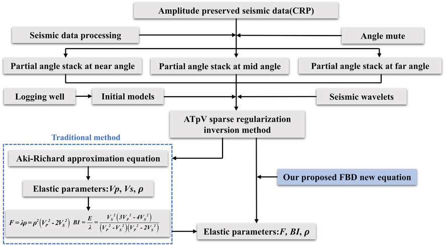
Figure 3. The workflow of the inversion method.

Algorithm 1.Inversion Pseudocode based on ADMM of the ATpV method.

Algorithm: Multitrace pre-stack inversion of elasticity parameters using ADMM and ISTA.

Input: seismic data $\mathit{d}$,initial model ${\mathit{r}}_{\mathit{0}}$, seismic wavelet w, difference matrix ${\mathit{D}}_x$, ${\mathit{D}}_y$ , parameter terms ${\mu }_1$, ${\mu }_2$, ${\mu }_3$, $\lambda$, $\eta$, $P$, error threshold ${\epsilon }_{\max }$.

Initial values: $k=0,{\mathit{r}}^{\left(0\right)}={\mathit{r}}_0,{\mathit{r}}_x={\mathit{r}}_{\mathrm{y}}={\mathit{C}}_x={\mathit{C}}_x=0.$

1. Updated ${\mathit{r}}^{\left(k+1\right)}$ by Equations 49, 50.

2. Updated ${{\mathit{r}}_x}^{\left(k+1\right)}$ , ${{\mathit{r}}_y}^{\left(k+1\right)}$ by Equations 53, 54.

3. Updated ${{\mathit{C}}_x}^{\left(k+1\right)}$ , ${{\mathit{C}}_{\mathrm{y}}}^{\left(k+1\right)}$ by Equations 58, 59.

4. If: $\frac{{‖{\mathit{r}}^{\left(k+1\right)}-{\mathit{r}}^{\left(k\right)}‖}_2}{{‖{\mathit{r}}^{\left(k+1\right)}‖}_2}\le {\epsilon }_{\max }$, get the inversion results.

Otherwise, increment k by 1 and repeat steps 1 through 4.

Output results: ${\left[\begin{array}{ccc}\mathit{F}& \mathit{B}\mathit{I}& \mathit{\rho }\end{array}\right]}^T=e^{{\mathit{r}}^{\left(k+1\right)}}$.

3 Numerical examples

3.1 Synthetic data test

To demonstrate the reliability and practicality of the simultaneous inversion method for fluid indicator and brittleness index presented in this paper, we conducted three sets of tests using synthetic seismic data derived from actual logging data. First, we obtained the multi-angle pre-stack seismic data by convolving the theoretical Ricker wavelet with the reflection coefficients computed from the actual log data based on the Zoeppritz equation, as shown in Figure 4. Then, to assess the performance of the inversion method under different noise conditions, we introduced various levels of random noise into the data. Moreover, Figures 4B, C show noisy datasets with SNR (Signal-to-Noise Ratio) of 5 and 2, respectively.

Figure 4

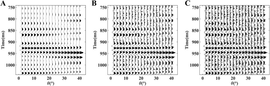
Figure 4. Synthesized seismic data, where (A) is noise-free, (B) SNR is 5, and (C) is 2.

Figures 5–7 present the results obtained from the synthetic data, the inverted data: fluid indicator F, brittleness index BI, and density (red solid curves), the initial models (green dashed curves), and the original well data (black solid curves), and the distribution of error between them. From Figure 5, in the noise-free case, all elastic parameter inversion results are well inverted and agree very well with the original well curve tracks. Figures 6, 7 show the inversion results when the SNR of the synthetic data is 5 and 2, respectively. We found that when the low-frequency curve is smooth and the model resolution is low, the gap between the obtained results and the actual logging data is more minor. The resolution of the inversion results can be guaranteed. Even at an SNR of 2, the inversion results obtained in this paper can also be matched well with the original well curves and have good noise resistance.

Figure 5

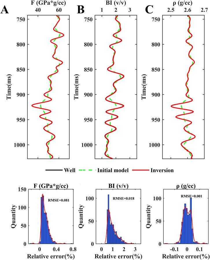
Figure 5. Inversion results from the noise-free synthetic data, along with error statistics and RMSE between them and the well data, where (A) is the fluid indicator, (B) is the brittleness index, and (C) is the density.

Figure 6

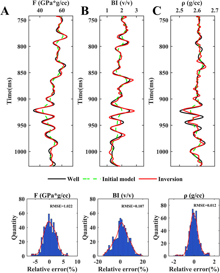
Figure 6. Inversion results from the synthetic data with SNR = 5, along with error statistics and RMSE between them and the well data, where (A) is the fluid indicator, (B) is the brittleness index, and (C) is the density.

Figure 7

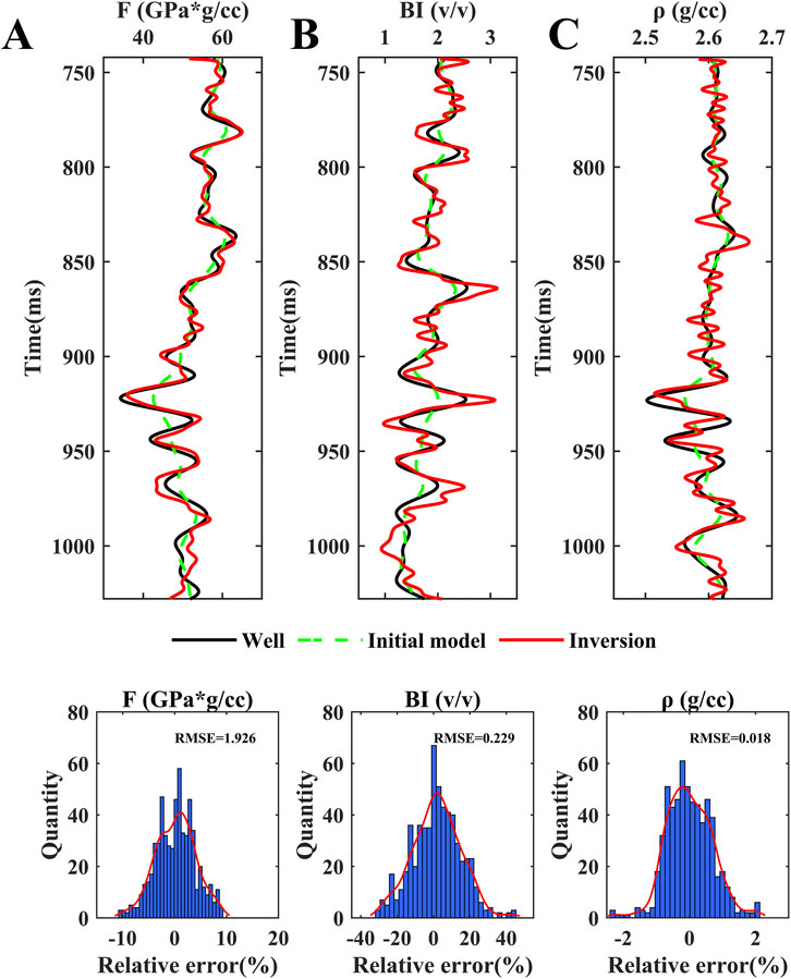
Figure 7. Inversion results from the synthetic data with SNR = 2, along with error statistics and RMSE between them and the well data, where (A) is the fluid indicator, (B) is the brittleness index, and (C) is the density.

Then, to quantitatively evaluate our results, we use Equations 60, 61 to calculate the inversion result errors $\epsilon$ and RMSE (root-mean-square-errors).

$\epsilon =\left(\frac{X_{inv}-X_{well}}{X_{well}}\right)\times 100\%(60)$

$RMSE=\sqrt{\frac{{\displaystyle \sum _{i=1}^N}{\left({X^i}_{inv}-{X^i}_{well}\right)}^2}{N}}(61)$

where X_inv and X_well represent the inversion result and original well curve, respectively. N is the number of sampling points.

We find that the inversion error for the brittleness index is more significant than that for the indicator index and density in the noise-free case. Still, the inversion error for all results is less than 5%, giving high accuracy. With the increase of noise, the inversion errors and RMSE of the brittleness index significantly increase. However, the errors and RMSE of fluid indicator and density vary within normal limits. Overall, the synthetic data test results can demonstrate that the methodology of this paper is theoretically feasible.

3.2 Field data application

The validity and practicability of the methodology proposed in this paper are verified through a field shale gas reservoir work area. This paper’s field study area (as shown in Figure 8) is located in the Sichuan Basin, China, and the primary target formation is the Silurian Longmaxi Formation. Well A in the work area drilled a high-quality shale gas reservoir, but the reservoir thickness is relatively small. The main target reservoir and lithology of well A are shown in Figure 9. The upper part of T1 is a limy siltstone with interbedded gray and sand. The section from T1 to T2 is a shale Section 1 with locally thinly interbedded argillaceous siltstone. The reservoir section from T2 to T3 is characterized by high porosity and substantial organic matter content, making it a high-quality, gas-bearing shale reservoir (Section 2) with significant hydrocarbon production potential. The lower part of T3 is the underlying limestone layer. In addition, based on actual logging curve values, such as elasticity curves for velocity and density, we can calculate the fluid indicator curve and brittleness index curve using Equations 3, 4. We can find that the fluid indicator curve and the brittleness index curve show apparent low-value and high-value anomalies in the shale 2 section; it is a favorable location for predicting shale reservoirs.

Figure 8

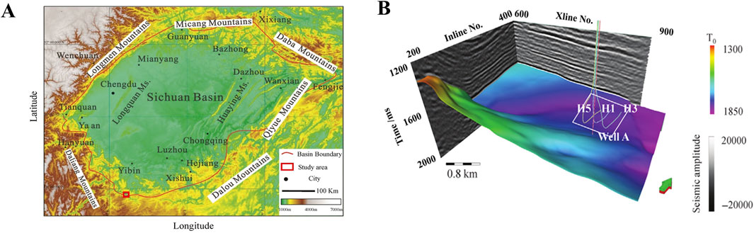
Figure 8. Specific information of the actual work area, where (A) is the location of the study area in the Sichuan Basin, (B) is a 3D display of the seismic data of the study area, where the formation is the basement of the Longmaxi Formation shale, and A is a straight well with logging information (Lin et al., 2022).

Figure 9

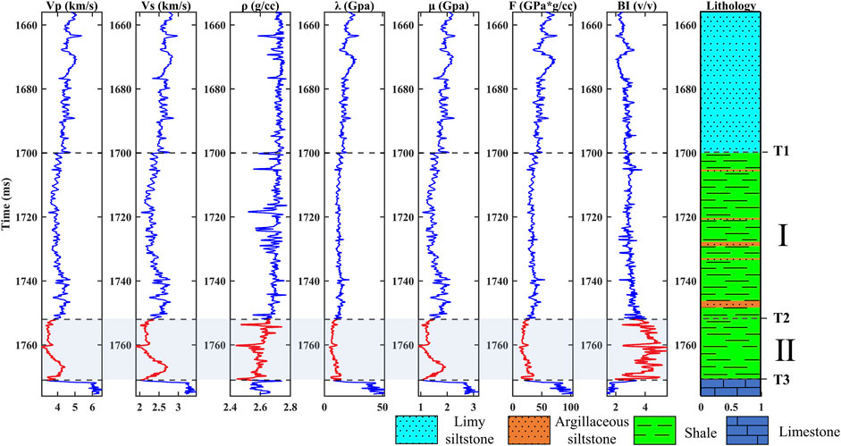
Figure 9. Original log curves, calculated fluid indicator and brittleness index curves, and lithologic distributions for well A. The red curves represent the high-quality reservoir Section 2.

Figure 10 shows the stacked seismic data with center incidence angles of 5° (0°–10°) in Figure 10A, 15° (10°–20°) in Figure 10B, and 25° (20°–30°) in Figure 10C, respectively. The profile has 285 traces of seismic data, and the red vertical line represents the path of well A, which is located on trace 112. In addition, the low-frequency components often lacking in the actual seismic data may lead to unstable inversion results. Therefore, a common approach is introducing initial model constraints in the inversion constraint term to make the results more reliable. Utilizing the seismic stratigraphic information, the fluid indicator, brittleness index, and density data from well A were extrapolated, interpolated, and then low-pass filtered to generate the corresponding low-frequency models, as illustrated in Figures 11A–C.

Figure 10

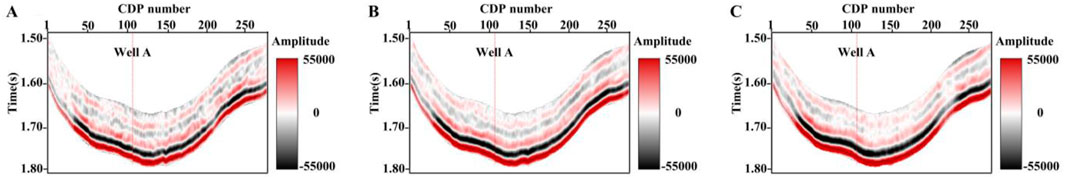
Figure 10. Stacked seismic data with different angle parts, where (A) is 0°–10°, (B) is 10°–20°, and (C) is 20°–30°.

Figure 11

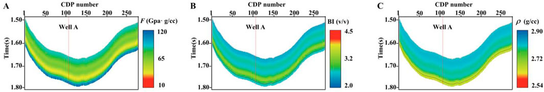
Figure 11. The initial model of the parameters to be inverted, where (A) is the fluid indicator, (B) is the brittleness index, and (C) is the density.

According to the inversion Algorithm 1 and combined with the approximate equation proposed in Equation 25, we inverted the 2D seismic data. Figures 12A–C shows the final 2D inversion results for the target parameters.

Figure 12

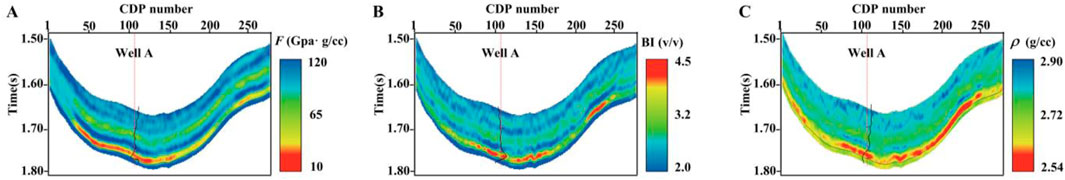
Figure 12. 2D simultaneous inversion results based on our proposed approximation equation, where (A) is the fluid indicator, (B) is the brittleness index, and (C) is the density.

In the fluid indicator inversion results, the red color indicates that the fluid identification factor is low, which means that the formation in the red part of the profile is likely to have fluids. In the brittleness index inversion results, the red color indicates high brittleness index values, which means that the formation in the red part of the profile is prone to fracture. Figure 12 shows that the brittleness inversion results have apparent high anomalies in the target layer section (T2 to T3). The fluid indicator inversion results have low anomalies in the target layer section (T2 to T3). The combination of the two inversion results indicates that the formation at this location is brittle and contains fluid, which is in agreement with the recognition in Figure 9. The combination of the inversion results is beneficial to characterize the gas-bearing shale reservoir better and helps us identify the target shale reservoir section.

To demonstrate the advantages and reliability of the direct inversion method for fluid indicator F and brittleness index BI proposed in this paper, we followed the inversion strategy outlined in Figure 3. Initially, according to the method proposed in this paper, we invert three elastic parameters $V_P$, $V_S$, and ρ, using the Aki-Richards approximation equation. Subsequently, we indirectly calculated the F and BI at the well location (trace 112) using Equations 3, 4, as illustrated by the green curves in Figure 13. Eventually, we extracted the inversion results of F and BI for the location of well A from Figure 12 and represented them as red curves in Figure 13.

Figure 13

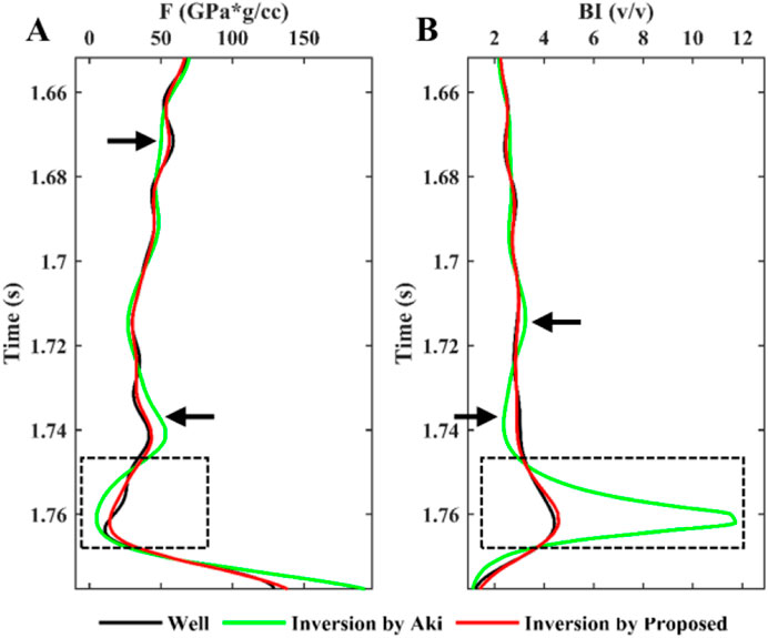
Figure 13. Inversion results of elasticity parameters based on the Aki-Richard equation in Equation 1 (green curve) and our proposed equation (red curve), where (A) is the fluid indicator and (B) is the brittleness index.

From Figures 13A, B, we found that the indirect inversion results accumulate errors in the calculation, which can lead to inaccurate results at the reservoir location (black dotted box). In addition, in several places in Figure 13 (black arrows), we can also find that the indirect prediction results (green solid curves) significantly exceed the actual well data (black solid curves). In contrast, the simultaneous inversion results for the fluid indicator and brittleness index (red solid curves) proposed in this paper strongly align with the original well curves. Furthermore, the residuals and RMSE analysis in Figure 14 indicate that the simultaneous inversion method yields much smaller residuals and lower RMSE than the indirect calculation method. Therefore, the approximation equation proposed in this paper enables more accurate and reliable simultaneous inversion of fluid indicator and brittleness index.

Figure 14

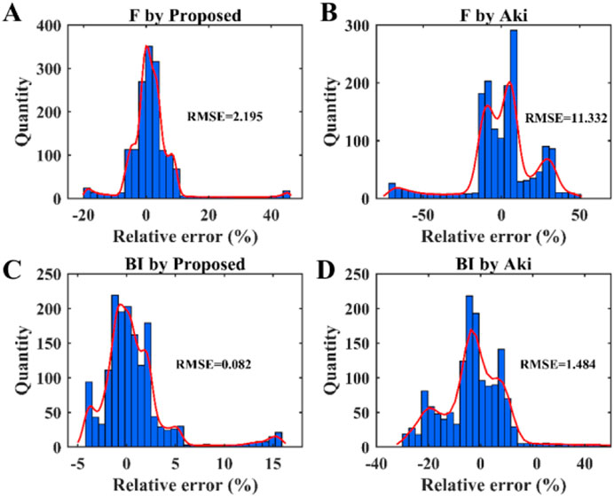
Figure 14. Error statistics and RMSE for inversion results from Aki-Richards and proposed equations, where (A) and (C) are fluid indicator and brittleness index by proposed equation in Equation 25, and (B) and (D) are by Aki in Equation 1.

The brittleness index BI, as an engineering sweet spot, is employed to characterize the fracturing ability of rock, which plays an instrumental guidance role in shale reservoir hydraulic fracturing construction, and the shale gas fluid indicator F, as a geological sweet spot has been revealed to be used to characterize hydrocarbon-bearing enriched zones. The combination of engineering and geological sweet spots is dedicated to the well deployment, horizontal well trajectory design, and effective shale gas production and extraction promotion. Based on the simultaneous seismic inversion method of shale gas fluid factor and brittleness index realized in this article, 3D pre-stacked seismic inversion at the fracturing platform has been utilized to perform the spatial distribution estimation with the above double-sweet spot parameters. The 3D seismic data was acquired by 230 Inlines and 270 Xlines, where wells H1, H3, and H5 are drilled as horizontal fractured wells in the shale reservoir, detecting numerous micro-seismic events at different periods. The inversion result slices of the fluid indicator and brittleness index along the destination layer are displayed in Figures 15A, B, respectively. The dashed circle closures pointed by white arrows reveal the hydrocarbon-enriched favorable fracturing zones, where the low fluid indicator spreading in Figure 15A represents enrichment of shale gas resources, and the high brittleness index distribution in Figure 15B represents satisfactory rock brittleness, which is beneficial to fracture fragmentation and facilitates hydraulic fracturing construction. The black dashed line Ft1 represents the projection of the seismic wave artificial fault interpretation conclusion on the slice. It can be seen that the fluid indicator exhibits uninteresting high values because the fault structure leads to increased stratum permeability, which is unfavorable to shale gas storage. The brittleness index presents low values, indicating that the rock brittleness at the fault location may be inferior because the fracture zone has been filled with more nonbrittle minerals, such as clay. In addition, in Figure 15C, numerous micro-seismic events in Figure 15D detected along three horizontal wells H1, H3, and H5 demonstrate the satisfying positive correlation with the high brittleness index in the fracturing favorable zone, which indicates that the rock is brittle enough and can be easily fractured to induce micro-seismic events. The practical application demonstrates that this article’s simultaneous seismic inversion method of fluid indicator and brittleness index can effectively provide reliable guidance information for unconventional shale gas production.

Figure 15

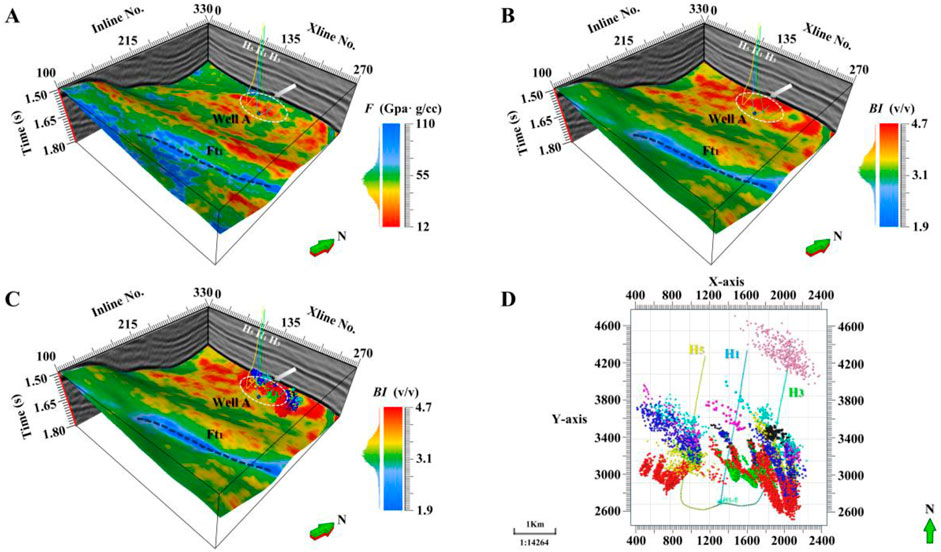
Figure 15. Slices of 3D seismic inversion prediction results along the destination layer in the study area, where (A) is a slice of brittleness index inversion result along the destination layer, (B) is a slice of fluid indicator inversion result along the destination layer, (C) is a slice of brittleness index inversion result and a superimposed display of micro-seismic events, and (D) is the micro-seismic events detected from three horizontal wells.

4 Discussion

In unconventional resource exploration, accurately identifying fluid indicators and brittleness indices in shale gas reservoirs is crucial for optimizing fracture zone selection and enhancing production efficiency. Traditional seismic methods typically rely on indirect calculation of sweet spot parameters, a process that is susceptible to various errors, resulting in unstable inversion outcomes and relatively low precision. In contrast, the synchronous seismic inversion method proposed in this study addresses the challenge of simultaneously inverting fluid indicators and brittleness indices, thereby avoiding the cumulative errors associated with indirect calculations.

To further improve the precision of the inversion results, this study introduced the ATpV inversion method based on L_P norm sparse constraint. Compared to conventional single-trace inversion methods, the proposed method demonstrates significant improvements in both computational efficiency and accuracy. Single-trace inversion methods typically involve the successive inversion of individual parameters, making them more vulnerable to noise. In contrast, the synchronous inversion method allows for the simultaneous estimation of multiple parameters, thereby reducing noise interference during the inversion process and enhancing the robustness and stability of the results. Validation using actual seismic data from the Sichuan Basin reveals that the fluid indicator λρ exhibits high sensitivity in fluid identification within shale gas reservoirs, while the brittleness index E/λ proves to be more effective in identifying gas-rich shale formations.

Overall, the proposed simultaneous inversion method and its new approximation equation, combined with the advantages of sparse regularization, not only overcome the limitations of traditional methods in shale gas exploration but also demonstrate strong stability and noise resistance in practical applications. However, there is still room for improvement. For instance, although the proposed method has shown good application results in shale gas reservoirs in the Sichuan Basin, its applicability in other geological conditions needs further validation. Future work will involve expanding the method’s applicability and enhancing practical data testing in different geological environments to improve its universality and reliability.

5 Conclusion

In exploring and developing unconventional resources, it is critical to accurately identify fluids in the reservoir and obtain a brittleness index that characterizes the brittleness of the reservoir rock. The fluid indicator λρ exhibits high sensitivity and robustness in detecting fluids within shale gas reservoirs. The brittleness index E/λ, is more effective than Young’s modulus in characterizing gas-rich shales. Higher brittleness in rocks typically corresponds to higher E/λ values. Consequently, the simultaneous inversion of pre-stack seismic data to obtain both fluid indicators and brittleness indices allows for more accurate prediction of “sweet spots” in shale gas reservoirs and the identification of favorable fracture zones.

In this paper, we derived a new approximate equation based on the Aki-Richards approximation under plane P-wave incidence. This equation consists of three components: fluid indicator λρ, brittleness index E/λ, and density ρ. Model tests have shown that the accuracy of this new approximation equation meets the requirements for practical applications, thus laying a theoretical foundation for the pre-stack inversion to obtain λρ and E/λ. Building on this foundation, we propose an ATV sparse inversion method based on L_P norm constraint to obtain these two parameters stably. This method avoids the cumulative errors introduced by indirectly calculating the sweet spot parameters and can obtain more accurate inversion results.

Finally, based on model tests and practical applications in the gas-bearing shales of the Silurian Longmaxi Formation, the proposed approximate equation combined with sparse regularization for simultaneous inversion has demonstrated excellent stability and noise resistance. The inversion results are reasonable and reliable, which can be a valuable guide for locating the sweet spot of shale gas reservoirs in practical situations.

Data availability statement

The datasets presented in this article are not readily available because Field data associated with this research are confidential and cannot be released. Requests to access the datasets should be directed to CL, MTU1Mzc4NTA0OUBxcS5jb20=.

Author contributions

CL: Conceptualization, Data curation, Investigation, Methodology, Software, Writing – original draft. XW: Project administration, Resources, Supervision, Writing – review and editing. YZ: Validation, Writing – original draft. BL: Data curation, Resources, Writing – review and editing. YQZ: Formal Analysis, Software, Writing – original draft.

Funding

The author(s) declare that financial support was received for the research and/or publication of this article. This work is supported by the National Natural Science Foundation of China (Grant Nos. 42304147), Postdoctoral Fellowship Program (Grant Nos. GZC20230326), and the China Postdoctoral Science Foundation (Grant Nos. 2024MF750281).

Conflict of interest

The authors declare that the research was conducted in the absence of any commercial or financial relationships that could be construed as a potential conflict of interest.

Generative AI statement

The author(s) declare that no Generative AI was used in the creation of this manuscript.

Publisher’s note

All claims expressed in this article are solely those of the authors and do not necessarily represent those of their affiliated organizations, or those of the publisher, the editors and the reviewers. Any product that may be evaluated in this article, or claim that may be made by its manufacturer, is not guaranteed or endorsed by the publisher.

References

Aki, K., and Richards, P. G. (2001). Quantitative seismology. Sausalito, CA: University Science Books.

Google Scholar

Buyanov, V. (2011). BP: statistical review of world energy. Econ. Policy 4, 38–55.

Google Scholar

Chartrand, W. R., and Yin, W. T. (2016). Splitting methods in communication, imaging, science, and engineering. Switzerland: Springer, 237–249. doi:10.1007/978-3-319-41589-5_7

CrossRef Full Text | Google Scholar

Chen, J. J., Zhang, G. Z., Chen, H. Z., and Yin, X. Y. (2014). “The construction of shale rock physics effective model and prediction of rock brittleness,” in 84th Annual International Meeting, SEG, Expanded Abstracts, 2861–2865. doi:10.1190/segam2014-0716.1

CrossRef Full Text | Google Scholar

Chi, X. G., and Han, D. H. (2006). Fluid property discrimination by AVO inversion. Tulsa, OK: Society of Exploration Geophysicists, 2052–2056. doi:10.1190/1.2369940

CrossRef Full Text | Google Scholar

Fatti, J. L., Smith, G. C., Strauss, P. J., and Levitt, P. R. (1994). Detection of gas in sandstone reservoirs using AVO analysis: a 3-D seismic case history using the Geostack technique. Geophysics 59, 1362–1376. doi:10.1190/1.1443695

CrossRef Full Text | Google Scholar

Ge, Z., Pan, S. L., Liu, J. X., Zhou, J. Y., and Pan, X. P. (2022). Estimation of brittleness and anisotropy parameters in transversely isotropic media with vertical axis of symmetry. IEEE Trans. Geosci. Remote Sens. 60, 1–9. doi:10.1109/TGRS.2021.3073162

CrossRef Full Text | Google Scholar

Gholami, A. (2015). Nonlinear multichannel impedance inversion by total-variation regularization. Geophysics 80, R217–R224. doi:10.1190/geo2015-0004.1

CrossRef Full Text | Google Scholar

Goodway, B., Chen, T., and Downton, J. (1997). “Improved AVO fluid detection and lithology discrimination using Lamé petrophysical parameters,” in “λρ,” “μρ,” “λμ fluid stack,” from P and S inversions (Tulsa, OK: Society of Exploration Geophysicists). doi:10.1190/1.1885795

CrossRef Full Text | Google Scholar

He, L. S., Wu, H., Wen, X. T., and You, J. (2022). Seismic acoustic impedance inversion using reweighted L1-norm sparse constraint. IEEE Geosci. Remote Sens. Lett. 19, 1–5. doi:10.1109/LGRS.2022.3168015

CrossRef Full Text | Google Scholar

Hedlin, K. (2000). Pore space modulus and extraction using AVO. Calgary: SEG Annual Meeting. doi:10.1190/1.1815749

CrossRef Full Text | Google Scholar

Jia, C., Zheng, M., and Zhang, Y. F. (2012). Unconventional hydrocarbon resources in China and the prospect of exploration and development. Pet. Explor. Dev. 39, 139–146. doi:10.1016/S1876-3804(12)60026-3

CrossRef Full Text | Google Scholar

Jin, X. C., Shah, S. N., Roegiers, J. C., and Zhang, B. (2015). Fracability evaluation in shale reservoirs-an integrated petrophysics and geomechanics approach. SPE J. 20, 518–526. doi:10.2118/168589-MS

CrossRef Full Text | Google Scholar

Kumar, V., Sondergeld, C. H., and Rai, C. S. (2012). Nano to macro mechanical characterization of shale. SPE Annu. Tech. Conf. Exhib. Richardson, TX: Society of Petroleum Engineers. doi:10.2118/159804-MS

CrossRef Full Text | Google Scholar

Li, H. (2022). Research progress on evaluation methods and factors influencing shale brittleness: a review. Energy Rep. 8, 4344–4358. doi:10.1016/j.egyr.2022.03.120

CrossRef Full Text | Google Scholar

Li, H. (2023). Advancing “Carbon Peak” and “Carbon Neutrality” in China: a comprehensive review of current global research on carbon capture, utilization, and storage technology and its implications. ACS Omega 45, 42086–42101. doi:10.1021/acsomega.3c06422

PubMed Abstract | CrossRef Full Text | Google Scholar

Li, L., Zhang, G. Z., Pan, X. P., Zhang, J. M., Zhu, Z. Y., Li, C., et al. (2022). Bayesian amplitude variation with angle and azimuth inversion for direct estimates of a new brittleness indicator and fracture density. Geophysics 87, M189–M197. doi:10.1190/geo2021-0767.1

CrossRef Full Text | Google Scholar

Lin, K., Zhang, B., Zhang, J. J., Fang, H. J., Xi, K. F., and Li, Z. (2022). Predicting the azimuth of natural fractures and in situ horizontal stress: a case study from the Sichuan Basin, China. Geophysics 87, B9–B22. doi:10.1190/geo2020-0829.1

CrossRef Full Text | Google Scholar

Liu, Z., and Sun, Z. (2015). New brittleness indexes and their application in shale/clay gas reservoir prediction. Pet. Explor. De. 42, 129–137. doi:10.1016/S1876-3804(15)60016-7

CrossRef Full Text | Google Scholar

Luan, X. Y., Di, B. R., Wei, J. X., Li, X. Y., Qian, K. R., Xie, J. Y., et al. (2014). Laboratory measurements of brittleness anisotropy in synthetic shale with different cementation. Seg. Expand. Abstr., 3005–3009. doi:10.1190/segam2014-0432.1

CrossRef Full Text | Google Scholar

Ma, Z. Q., Yin, X. Y., Li, K., Tan, Y. Y., Zhang, J. L., and Haimand, A. (2023). Fracture detection, fluid identification and brittleness evaluation in the gas-bearing reservoir with tilted transverse isotropy via azimuthal Fourier coefficients. Gas. Sci. Eng. 111, 2949–9089. doi:10.1016/j.jgsce.2023.204910

CrossRef Full Text | Google Scholar

Mullen, J. (2010). Petrophysical characterization of the eagle ford shale in South Texas. Can. Unconv. Resour. Int. Petroleum Conf. doi:10.2118/138145-MS

CrossRef Full Text | Google Scholar

Murphy, W., Reischer, A., and Hsu, K. (1993). Modulus decomposition of compressional and shear velocities in sand bodies. Geophysics 58, 227–239. doi:10.1190/1.1443408

CrossRef Full Text | Google Scholar

Ning, Z. H., He, Z. H., and Huang, D. J. (2006). Highly sensitive fluid identification based on seismic data. Geophys. Prospect. Pet. 45, 239–241. [in Chinese]. doi:10.3969/j.issn.1000-1441.2006.03.005

CrossRef Full Text | Google Scholar

Pan, X. P., Zhang, G. Z., and Chen, J. J. (2020). The construction of shale rock physics model and brittleness prediction for high-porosity shale gas-bearing reservoir. Pet. Sci. 17, 658–670. doi:10.1007/s12182-020-00432-2

CrossRef Full Text | Google Scholar

Quakenbush, M., Shang, B., and Tuttle, C. (2006). Poisson impedance. Lead. Edge 25, 128–138. doi:10.1190/1.2172301

CrossRef Full Text | Google Scholar

Rickman, R., Mullen, M. J., Petre, J. E., Grieser, B., and Donald, K. (2008). A practical use of shale petrophysics for stimulation design optimization: all shale plays are not clones of the Barnett Shale. SPE Annu. Tech. Conf. Exhib. doi:10.2118/115258-MS

CrossRef Full Text | Google Scholar

Russell, B. H., Gray, D., and Hampson, D. P. (2011). Linearized AVO and poroelasticity. Geophysics 76, 19–29. doi:10.1190/1.3555082

CrossRef Full Text | Google Scholar

Russell, B. H., Hedlin, K., Hilterman, F. J., and Lines, L. R. (2003). Fluid-property discrimination with AVO: a Biot-Gassmann perspective. Geophysics 68, 29–39. doi:10.1190/1.1543192

CrossRef Full Text | Google Scholar

Sharma, R. K., and Chopra, S. (2015). Determination of lithology and brittleness of rocks with a new attribute. Lead. Edge 34, 554–564. doi:10.1190/tle34050554.1

CrossRef Full Text | Google Scholar

Shuey, R. T. (1985). A simplification of the Zoeppritz equations. Geophysics 50, 609–614. doi:10.1190/1.1441936

CrossRef Full Text | Google Scholar

Smith, G. C., and Gidlow, P. M. (1987). Weighted stacking for rock property estimation and detection of gas. Geophys. Prospect 35, 993–1014. doi:10.1111/j.1365-2478.1987.tb00856.x

CrossRef Full Text | Google Scholar

Sun, Y. C., Chen, S. W., Li, Y. F., Zhang, J., and Gong, F. H. (2021). Shale rocks brittleness index prediction method using extended elastic impedance inversion. J. Appl. Geophy 188, 104–314. doi:10.1016/j.jappgeo.2021.104314

CrossRef Full Text | Google Scholar

Wen, X. T., Zhao, Y., Xie, C. L., and Li, C. L. (2024). Direct seismic inversion of a novel brittleness index based on petrophysical modeling in shale reservoirs. IEEE Trans. Geosci. Remote Sens. 62, 1–15. doi:10.1109/TGRS.2024.3436896

CrossRef Full Text | Google Scholar

Wu, H., He, Y. M., Chen, Y. P., Li, S., and Peng, Z. (2020). Seismic acoustic impedance inversion using mixed second-order fractional ATpV regularization. IEEE Access 8, 3442–3452. doi:10.1109/ACCESS.2019.2962552

CrossRef Full Text | Google Scholar

Yilmaz, Ö. (2001). Seismic data analysis: processing, inversion, and interpretation of seismic data. Soc. Explor. Geophys. doi:10.1190/1.9781560801580

CrossRef Full Text | Google Scholar

Yin, X. Y., Liu, X., and Zong, Z. Y. (2015). Pre-stack basis pursuit seismic inversion for brittleness of shale. Pet. Sci. 12, 618–627. doi:10.1007/s12182-015-0056-3

CrossRef Full Text | Google Scholar

Zhang, F. Q., Jin, Z. J., Sheng, X. J., Li, X. S., Shi, J. Y., and Liu, X. Q. (2017a). A direct inversion for brittleness index based on GLI with basic-pursuit decomposition. Chin. J. Geophys 60, 3954–3968. [in Chinese]. doi:10.6038/cjg20171023

CrossRef Full Text | Google Scholar

Zhang, G. Z., Du, B. Y., and Li, H. S. (2014). The method of joint pre-stack inversion of PP- and P-SV waves in shale gas reservoirs. Chin. J. Geophys 57, 4141–4149. [in Chinese]. doi:10.6038/cjg20141225

CrossRef Full Text | Google Scholar

Zhang, S., Huang, H. D., Dong, Y. P., Yang, X., Wang, C., and Lou, Y. N. (2017b). Direct estimation of the fluid properties and brittleness via elastic impedance inversion for predicting sweet spots and the fracturing area in the unconventional reservoir. J. Nat. Gas. Sci. Eng. 45, 415–427. doi:10.1016/j.jngse.2017.04.028

CrossRef Full Text | Google Scholar

Zhao, L., Lin, K., Wen, X. T., and Zhang, Y. Q. (2023). Anisotropic total variation pre-stack multitrace inversion based on Lp norm constraint. J. Pet. Sci. Eng. 220, 111–212. doi:10.1016/j.petrol.2022.111212

CrossRef Full Text | Google Scholar

Zhao, Y., Wen, X. T., Li, C. L., Xie, C. L., and Liu, Y. (2024). Systematic prediction of the gas content, fractures, and brittleness in fractured shale reservoirs with TTI medium. Pet. Sci. 21, 3202–3221. doi:10.1016/j.petsci.2024.04.015

CrossRef Full Text | Google Scholar

Zong, Z. Y., Yin, X. Y., and Wu, G. Z. (2012a). AVO inversion and poroelasticity with P- and S-wave moduli. Geophysics 77, N17–N24. doi:10.1190/geo2011-0214.1

CrossRef Full Text | Google Scholar

Zong, Z. Y., Yin, X. Y., and Wu, G. Z. (2012b). Elastic impedance parameterization and inversion with Young’s modulus and Poisson’s ratio. Geophysics 78, N35–N42. doi:10.1190/geo2012-0529.1

CrossRef Full Text | Google Scholar

Zong, Z. Y., Yin, X. Y., and Zhang, F. C. (2012c). Reflection coefficient equation and pre-stack seismic inversion with Young’s modulus and Poisson ratio. Chin. J. Geophys 55, 3786–3794. [in Chinese]. doi:10.6038/j.issn.0001-5733.2012.11.025

CrossRef Full Text | Google Scholar