Spatial distribution prediction of pore pressure based on Mamba model

Introduction: The pore pressure of formations is a critical factor in assessing reservoir stability, designing drilling programs, and predicting production dynamics. Traditional methods often rely on limited well-logging data and empirical formulas to derive one-dimensional formation pressure models, which are inadequate for accurately reflecting the three-dimensional distribution of pore pressure in complex geological structures.

Methods: To address this challenge, this study leverages the temporal characteristics of well-logging and seismic data, employing the Mamba technique in conjunction with high-precision seismic inversion results, to construct a pore pressure prediction model. The model is a structured state-space model designed to process complex time-series data, and improve efficiency through parallel scan algorithm, making it suitable for large-scale three-dimensional data prediction. Initially, the deep learning model is trained and optimized by collecting and analyzing well-logging data, including key parameters such as acoustic time difference and density. Advanced seismic inversion techniques are then employed to obtain three-dimensional elastic properties like subsurface velocity and density, which serve as input features for the trained deep learning model.

Results: Through complex nonlinear mappings, the model effectively captures the intrinsic relationship between input attributes and formation pressure, enabling accurate spatial distribution prediction of formation pore pressure. Research findings indicate that this method not only achieves high-precision formation pressure predictions but also reveals lateral variations in pore pressure that are challenging to detect using traditional methods.

Discussion: This provides robust technical support for the precise management and efficient development of oil and gas fields. With this method, oilfield engineers can more accurately assess formation pressure, optimize drilling programs, reduce accident risks, and enhance production efficiency.

1 Introduction

Pore pressure holds a fundamental position as a vital technical data in the intricate design and meticulous execution of drilling engineering endeavors, and carbon capture, utilization, and storage (CCUS). Furthermore, it serves as a critical parameter in the broader context of oil and gas field development, playing an indispensable role in the exploration and exploitation of hydrocarbon resources (Zong et al., 2024). On one hand, precise prediction of formation pressure is indispensable for determining an appropriate wellbore structure. It allows for proactive measures in zones with abnormal pressure, aids in designing suitable drilling fluid densities, ensures the stability of the wellbore, and plays a crucial role in preventing and controlling well surges, leaks, and collapses during the drilling process (Hussain and Ahmed, 2018). These measures, in turn, simplify subsurface complexities and bolster safety, ultimately contributing to the enhancement of mechanical drilling speeds. On the other hand, the formation pressure within oil and gas reservoirs significantly influences the properties of hydrocarbons. It dictates the methodologies employed for hydrocarbon development, the technical specifications, and the economic costs associated with extraction. Moreover, it has a profound impact on the ultimate recovery rates, making it a pivotal factor in the overall efficiency and profitability of oil and gas operations (Hazra et al., 2024; Ahmed et al., 2024b).

Pore pressure, alternately referred to as formation pressure, represents the force exerted upon the fluids residing within the pores of a rock formation. This pressure is typically correlated with the depth of the formation and is commonly expressed in terms of the static water pressure corresponding to the formation water column extending up to the surface (Chopra and Huffman, 2006). It is measured using units such as megapascals (MPa) or pounds per square inch (psi) and is denoted by the symbol $Pp$. Abnormal formation pressure can manifest in two primary forms: overpressure and underpressure. Overpressure arises when the pore pressure surpasses normal levels due to additional pressure sources, potentially resulting in hazardous incidents such as blowouts. The upper threshold of abnormally high pressure aligns approximately with the overburden pressure. Conversely, underpressure signifies a pore pressure that falls below normal levels, which can lead to issues including well leakage, circulation losses, and differential pressure sticking, ultimately escalating drilling costs (Greenwood et al., 2009).

In the field of engineering, the prediction of pore pressures can be divided into direct and indirect methodologies. Direct methods encompass techniques such as leak-off tests, and rock mechanics experiments, both aimed at measuring formation pressures directly. Nonetheless, these methods generally offer measurements solely at specific depths within the well, posing challenges in obtaining continuous pore pressure profiles or volumes. Furthermore, the process of collecting downhole data is not only costly but also entails risks such as drillstring sticking or loss during the collection phase. Currently, the most prevalent approach involves the indirect prediction of pore pressure through the utilization of mechanistic models (Qi et al., 2024). When utilizing the theory of undercompaction for predicting formation pressure, it is indispensable to employ the normal compaction background trend, which is commonly derived from stable lithological combinations, minimal structural impacts, and assumptions of limited heterogeneity. However, in practical applications, accurately establishing the normal compaction trend line often presents significant challenges and is inherently subjective (Sanei et al., 2023).

The second approach is the effective stress method, which indirectly predicts pore pressure by calculating the overburden pressure and effective stress. This method eliminates the need to establish a normal compaction trend line and thus avoids the associated prediction errors that arise from inaccuracies in this trend. Its advantage lies in bypassing the complexities inherent in normal compaction trends, thereby simplifying application. However, the implementation of this method relies on several assumptions, and its accuracy in predicting pressure depends significantly on the specific conditions of the study area and the degree of alignment with these assumptions. A common feature of these methods is their reliance on a relatively straightforward formula that primarily uses the P-wave velocity of the formation. Nevertheless, these methods overlook a crucial aspect: S-wave velocity and density of the formation are also closely related to pore pressure. Many rock physics studies have shown that the variation of S- wave velocity is almost entirely related to the stress on the rock matrix, and rock density reflects the changes in the internal structure of the rock when subjected to pore pressure (MacBeth, 2004; Ahmed et al., 2024a), while P-wave velocity is significantly affected by the depth of the pore fluid (Soares et al., 2024). When using this method and relying solely on P-wave velocity to predict pore pressure, there is a tendency to misunderstand the decrease in fluid velocity as the influence of rock matrix stress, ultimately resulting in predicted pore pressure values exceeding actual values. Therefore, by introducing S-wave velocity and density as additional variables, the influence of pore pressure on rock physical properties can be better reflected, and the accuracy of pore pressure prediction can be improved.

Mylnikov et al. (2021) believed that traditional approaches have encountered a dilemma in improving accuracy, which may be attributed to two main reasons. On the one hand, there is an inherent discrepancy between empirical models and fundamental physical principles. On the other hand, there is a challenge in selecting a parameter combination within the standard analytical model that aligns the predicted pressure with the comprehensive set of actual field data (pore pressure measurements).

With the relentless advancement of machine learning technology, we anticipate the development of more efficient, precise, and secure methodologies for predicting pore pressure, thereby providing oil/gas engineering with even more reliable technical support. Unlike traditional mechanistic models, data-driven models offer simpler establishment processes and robust adaptability, transcending limitations posed by data types, scales, and dimensions. These models excel at handling a wide variety of diverse, voluminous, and complex data relevant to drilling engineering.

Consequently, research on the application of machine learning in predicting the pore pressures within geological formations holds exceptionally vast application prospects and is of paramount significance (Radwan et al., 2022). Syed et al. (2022) have thoroughly discussed machine learning techniques developed in the past decades and tested them to enhance the accuracy of petrophysical and geomechanical simulation models. They believe that the application of machine learning to predict mechanical properties represents an indispensable path forward. Various studies have explored this domain, including Keshavarzi and Jahanbakhshi (2013), who used a backpropagation neural network (BPNN) and generalized regression neural network (GRNN) to predict the pressure gradient of the Asmari oilfield in Iran by incorporating depth, permeability, rock density, and porosity as inputs. Aliouane et al. (2015) proposed a model combining fuzzy logic and artificial neural networks for predicting pore pressure in shale gas reservoirs. Huang et al. (2022) propose a machine learning method to indirectly predict pore pressure based on the effective stress theorem.

Hadi et al. (2019) introduced an artificial neural network method for forecasting formation pressure, leveraging mechanical and logging parameters such as vertical depth, density, neutron porosity, natural gamma, acoustic time difference, and uniaxial compressive strength. Ahmed S. A. et al. (2019) employed diverse machine learning algorithms based on well logging data and surface drilling parameters to predict formation pressure and fracture pressure, with the support vector machine emerging as the most accurate. Farsi et al. (2021) utilized a multi-layer extreme learning machine and optimization algorithm to predict the formation pore pressure of carbonate reservoirs, achieving results that surpassed the predictive performance of traditional physical models. Zhang et al. (2022) optimized nine logging parameter variables through feature selection and applied various machine learning algorithms, such as decision trees, to predict formation pressure, with the decision tree algorithm demonstrating robust generalization ability on the test set. Soares et al. (2024) combined the K-nearest neighbor and geostatistical seismic inversion to obtain the 3D volumes of pore pressures. Krishna et al. (2024) compared several commonly used methods and analyzed their performance for pore pressure prediction based on well logging data (Ahmed et al., 2024a; Ahmed et al., 2024b). Among them, the random forest method performs the best.

Haris et al. (2017) employed probabilistic neural networks (PNN) to forecast pore pressure distribution, utilizing both pre-stack and post-stack seismic data from the South Sumatra oil field. Hutomo et al. (2019) established a reservoir pore pressure prediction model using artificial neural networks, informed by three-dimensional seismic data including acoustic impedance, shear impedance, seismic frequency, and amplitude. Naeini et al. (2019) introduced a supervised deep neural network method, creating a neural network capable of directly predicting crucial rock properties based on seismic inversion results. Then, Andrian et al. (2020) utilized an adaptive neuro-fuzzy inference system to predict pore pressure distribution from two-dimensional seismic data within the study area. Zhang et al. (2024) found that most traditional deep learning models are less effective in addressing generalization issues, especially for predicting 3D pore pressure.

The propagation of seismic waves constitutes a continuous and unceasing process, whereas seismic recorders meticulously gather data at precise, often millisecond, intervals. Each data point, anchored to a specific time step, is intricately linked to its predecessor, fostering a temporal dependency that shapes a distinctive and characteristic temporal data structure (Yilmaz, 2001; Liu et al., 2023). Logging data involves the use of instruments to measure the physical and chemical properties of rock formations at various depths during the drilling process, thereby reflecting changes in subsurface geological structures as they relate to depth. Essentially, logging data consists of sequential information gathered depth-by-depth. However, since drilling is a continuous process over time, logging data is also intrinsically tied to temporal factors (Pham et al., 2020). Cao et al. (2024) pointed out that the existing machine learning methods often struggle to capture the intrinsic temporal dynamics of the data, resulting in suboptimal prediction accuracy. In order to effectively consider the temporal characteristics of geological data such as logging and seismic data, we propose introducing the Mamba model for 3D pore pressure prediction. The Mamba model represents a groundbreaking approach to linear time series modeling, elegantly blending the prowess of recurrent neural networks (RNNs) (Hochreiter and Schmidhuber, 1997) and convolutional neural networks (CNNs) (LeCun et al., 1998) to tackle the computational inefficiencies associated with processing extended sequences (Gu and Dao, 2023). By seamlessly integrating RNN’s sequential processing prowess with CNN’s global context-awareness within the framework of a State Space Model (SSM) (Voelker and Eliasmith, 2018; Gedon et al., 2020), Mamba achieves a meticulously balanced design. The Mamba model dynamically selects relevant state information and extracts features of the complex nonlinear trends in pore pressure with depth (or time) variations. It effectively captures long-term dependencies, enabling it to identify gradual manifestations of abnormal pressure events across multiple layers. This enhances the generalization without suffering from gradient vanishing issues, which are common in RNNs. Furthermore, logging and seismic data often span extensive depths or time periods, leading to lower computational efficiency in traditional models, Mamba achieves efficient parallel computing to ensure real-time predictive performance.

In the following section, we introduce the key features and basic structure of the Mamba model and extend its application to predict pore pressure. We demonstrate the feasibility of the method through two examples, and finally, we discuss the findings and draw conclusions.

2 Theory and methods

Strata and their properties exhibit temporal characteristics on a large time scale, reflecting long-term geological processes and changes. Both logging data and seismic data record physical quantities related to geological properties that change over time and display distinct temporal characteristics. Therefore, they can all be regarded as time series. State Space Models (SSMs) can be utilized to represent the state of a sequence at each time step and predict its next state based on the input model. By capturing the dynamic evolution of time series, SSMs provide a robust framework for both modeling and forecasting sequences (Gu and Dao, 2023; Dao and Gu, 2024). The Mamba model is an improved version of SSM, which mainly weakens the two assumptions of SSMs to better handle nonlinear and time-varying sequence data.

2.1 State-space model, SSM

The core of State Space Models (SSMs) lies in identifying an appropriate state representation that can be combined with the input sequence to accurately predict the output sequence. An SSM comprises two primary components:

The first one is the state equation, expressed as:

$h^{\prime }\left(t\right)=\mathbf{A}\left(t\right)h\left(t\right)+\mathbf{B}\left(t\right)x\left(t\right),(1)$

where $x(t)$ represents the input sequences. $h(t)$ denotes the hidden state representation at time $t$, which contains the current state information of the system. $h^{\prime }(t)$ represents the rate of change or derivative of the latent state vector at time $t$, indicating the change of the state over time. $\mathbf{A}$ is the state transition matrix, which describes how the hidden state updates itself over time. It determines the impact of the current state on state changes. $\mathbf{B}$ is the input matrix that describes how the input affects state changes. It determines the contribution of input to state changes. This equation describes the dynamics of the system by detailing how the state evolves from one time step to the next. It captures the internal mechanisms and transitions within the system, providing a mathematical framework for understanding the underlying processes.

The second one is the observation equation, expressed as:

$y\left(t\right)=\mathbf{C}\left(t\right)h\left(t\right)+\mathbf{D}\left(t\right)x\left(t\right),(2)$

where $y(t)$ represents the output vector, i.e., pore pressure, which is the response of the model to input and internal state. $\mathbf{C}$ is the output matrix that describes how the hidden state is mapped to the output, and it determines the direct impact of the current state on the output. $\mathbf{D}$ is the direct transfer matrix, which describes how the input directly affects the output and determines the direct contribution of the input to the output. In general, $\mathbf{D}$ is similar to skip connections, SSM is usually considered as the part that does not contain the skip connection. The structure of SSM is displayed in Figure 1. This equation specifies how the observable data (or measurements) are generated from the system’s state. It bridges the gap between the hidden state variables and the actual observations, allowing us to relate the internal state of the system to the external data we can measure. In the proposed method for the pore pressure prediction, the input includes the elastic attributes and time. The corresponding output is the pore pressure.

Figure 1

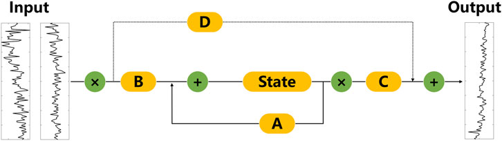
Figure 1. The structure of SSM.

In the above expression, both the input and output are continuous functions of time. However, since logging data and seismic data are obtained through discrete sampling, Equations 1, 2 should be discretized before applying. To adapt the continuous-time state space model to discrete input data, the SSM model employs a discretization process using the Zero Order Hold (ZOH) method. The process is as shown in Equations 3, 4. Gu et al. (2021), i.e.,

$\bar{\mathbf{A}}=\exp \left(\mathrm{\Delta }\mathbf{A}\right),(3)$

$\bar{\mathbf{B}}={\left(\mathrm{\Delta }\mathbf{A}\right)}^{-1}\left(\exp \left(\mathrm{\Delta }\mathbf{A}\right)-\mathbf{I}\right)\mathrm{\Delta }\mathbf{B},(4)$

where $\mathrm{\Delta }$ is a newly introduced learnable parameter representation called step size. Then we can obtain:

$h_k=\bar{\mathbf{A}}{h}_{k-1}+\bar{\mathbf{B}}{x}_k,(5)$

$y_k=\bar{\mathbf{C}}{h}_k,(6)$

where $h_k$ represents the latent state vector at the discrete time $k$. $h_{k-1}$ represents the latent state vector at the previous discrete time $k-1$. $\bar{\mathbf{A}}$ and $\bar{\mathbf{B}}$ denote the discretized state transition and input matrices. It can be seen that the current state is obtained by the combined action of the previous state and the current input through their respective discretization matrices $\bar{\mathbf{A}}$ and $\bar{\mathbf{B}}$. Similarly, $\bar{\mathbf{C}}$ denotes the discretized output matrix. The output is a linear transformation of the state. Because the output is a direct observation of the state and discretization do not change this relationship, $\bar{\mathbf{C}}$ is equal to $\mathbf{C}$. Overall, we can consider discretization as the first step in computing graphs in SSM forward propagation. It converts continuous parameters into discrete parameters so that downstream calculations only use $(\bar{\mathbf{A}},\bar{\mathbf{B}})$. This discretization strategy ensures that the model can maintain stable performance and accuracy when processing discrete time series Gu et al. (2021).

Note that the hidden state will be updated at each time step. $h_k$ is always updated under the joint action of $=\bar{\mathbf{A}}{h}_{k-1}$ and $\bar{\mathbf{B}}{x}_k$, it can be processed by the structure of Recurrent Neural Network (RNN). RNN relies solely on the hidden state from the previous step and the current input data, avoiding the need to recalculate the entire historical hidden state of the sequence. This characteristic makes RNN faster during inference and forecasting. However, this efficiency comes with the trade-off of longer training cycles, which is a significant drawback.

It is particularly important to note that when substituting Formula 5 into Formula 6, We can obtain Equations 7-10, which is similar to the calculation process of the convolution kernel

$y_k=\mathbf{C}\left(\bar{\mathbf{A}}{h}_{k-1}+\bar{\mathbf{B}}{x}_k\right),(7)$

$=\mathbf{C}\left(\bar{\mathbf{A}}\left(\bar{\mathbf{A}}{h}_{k-2}+\bar{\mathbf{B}}{x}_{k-1}\right)+\bar{\mathbf{B}}{x}_k\right)(8)$

$=\dots$

$=\mathbf{C}{\bar{\mathbf{A}}}^k\bar{\mathbf{B}}{x}_0+\mathbf{C}{\bar{\mathbf{A}}}^{k-1}\bar{\mathbf{B}}{x}_1+\mathbf{C}{\bar{\mathbf{A}}}^{k-2}\bar{\mathbf{B}}{x}_2+\cdots +\mathbf{C}\bar{\mathbf{B}}{x}_k.(9)$

Let $K=(\mathbf{C}{\bar{\mathbf{A}}}^k\bar{\mathbf{B}},\mathbf{C}{\bar{\mathbf{A}}}^{k-1}\bar{\mathbf{B}},\mathbf{C}{\bar{\mathbf{A}}}^{k-2}\bar{\mathbf{B}},\dots ,\mathbf{C}\bar{\mathbf{B}})$, denoting a kernel function, the output can be calculated by:

$y_k=\left(\mathbf{C}{\bar{\mathbf{A}}}^k\bar{\mathbf{B}},\mathbf{C}{\bar{\mathbf{A}}}^{k-1}\bar{\mathbf{B}},\mathbf{C}{\bar{\mathbf{A}}}^{k-2}\bar{\mathbf{B}},\dots ,\mathbf{C}\bar{\mathbf{B}}\right)\begin{array}{c}\hfill \left(\begin{array}{c}\hfill x_0\hfill \\ \hfill x_1\hfill \\ \hfill x_2\hfill \\ \hfill ⋮\hfill \\ \hfill x_k\hfill \end{array}\right)\hfill \end{array}.(10)$

That is to say, the output of SSM can be calculated using a convolution operation. One major advantage of representing SSM as a convolution is that it can be trained in parallel, similar to a CNN. However, due to the fixed kernel size, the inference or prediction speed of convolutional SSMs is generally not as fast as that of RNNs. In summary, recursive SSM excels in efficient inference capabilities, while convolutional SSM is favored for the parallelizable training process. By leveraging these different representations, one can flexibly choose the most suitable model based on the specific task requirements. During the training phase, the convolutional representation can be selected to achieve parallelization, enhancing training efficiency. In the inference stage, switching to the recursive representation can ensure faster response times.

2.2 Mamba model

One of the key challenges with SSM is that the aforementioned matrices ($\mathbf{A},\mathbf{B}$, and $\mathbf{C}$) do not adapt to different inputs, making it difficult to make targeted inferences based on the input data. This limitation is particularly pronounced in scenarios where models need to flexibly focus on or ignore specific inputs, as the static nature of these matrices restricts the capabilities of the model. Specifically, for general SSM models, the model receives input data and attempts to predict the output during training. The parameters of the model, represented by the values in matrices $\mathbf{A},\mathbf{B}$, and $\mathbf{C}$, are adjusted through optimization algorithms such as gradient descent in each iteration to minimize prediction errors. As training progresses, the values of these matrices gradually change to better fit the training data. Once the model training is complete and the model enters the prediction step, the values of matrices $\mathbf{A},\mathbf{B}$, and $\mathbf{C}$ are fixed to the values learned during the final stages of training. During inference, the model uses these fixed matrices to process new input data and generate predictions. The reason is mainly because of the two strong assumptions of SSM, i.e., linear and time invariant, while most actual systems are nonlinear and time-varying. This fixed nature of the matrices in SSM limits their flexibility and adaptability, especially in dynamic environments where the model needs to respond to varying input conditions. Mamba is essentially an improvement of the SSM model, freeing up these two assumptions.

The selective mechanism of Mamba elegantly refines its operation through the dynamic adjustment of the parameter matrix, achieved via the introduction of a selective weight vector, denoted as $\mathbf{s}$. This vector is meticulously computed to reflect the significance of the input data, thereby enhancing the adaptability and precision in response to varying input conditions. s is calculated by neuralnetworks, calculation process is as shown in Equation 11, i.e.,

$\mathbf{s}=\sigma \left(f_{\theta }\left(x_t\right)\right),(11)$

where $\sigma$ is the activation function, $f_{\theta }$ is the parameterization function of the neural network, and $\theta$ represents the parameters of the network. Then, the dynamic parameter matrix can be written as Equations 12-14:

$\mathbf{A}\left(x_t,\mathbf{s}\right)=f_{\theta }^{\mathbf{A}}\left(x_t,\mathbf{s}\right),(12)$

$\mathbf{B}\left(x_t,\mathbf{s}\right)=f_{\theta }^{\mathbf{B}}\left(x_t,\mathbf{s}\right),(13)$

$\mathbf{C}\left(x_t,\mathbf{s}\right)=f_{\theta }^{\mathbf{C}}\left(x_t,\mathbf{s}\right).(14)$

In this process, $\mathrm{\Delta }$ also becomes learnable. It determines the degree of variation of selective weights at each time step, thereby affecting the sensitivity and adaptability of the model to input data. The introduction of learnable $\mathrm{\Delta }$ allows the model to dynamically adjust the time interval based on data features. In this way, the model can preserve the temporal dependence between different time steps to a greater extent, thereby enhancing the model’s expressiveness Yu et al. (2018). A larger $\mathrm{\Delta }$ value can make the model more sensitive to input changes, which is equivalent to making the model focus more on the current input rather than the previous state, equivalent to selecting the current input and forgetting the current state. When $\mathrm{\Delta }$ is small, the model maintains the persistence of the existing state h and pays less attention to the current input.

Although the Mamba model does not change its parameters during inference, the selective mechanism introduced in its design allows the model to treat different inputs differently based on their characteristics, which is a significant improvement compared to the SSM. This selectivity is achieved through parameter learning during the training phase (different inputs are processed differently based on the parameters learned during the training phase).

Since matrices $\mathbf{A},\mathbf{B}$, and $\mathbf{C}$ are now dynamic, we cannot use convolutional representations to compute them (CNN requires a fixed kernel). Therefore, we can only use cyclic representations, which results in the loss of the parallel training capability provided by convolution. The Mamba model introduces a parallel scan algorithm, which paves the way for ultimate parallelization. This innovation hinges on the assumption that the order of operations is independent of their associative properties, allowing segments of a sequence to be computed separately and then iteratively combined. The selective state model within Mamba further distinguishes itself by enabling the differentiation between primary and secondary states, thus selectively focusing on significant samples. This mechanism effectively minimizes the interference from irrelevant noise, directing the model’s attention to valuable information, thereby enhancing overall performance. Compared to frameworks that adopt a global state modeling approach, the selective state model offers a more targeted strategy, significantly improving inference accuracy when tackling complex systems Gu and Dao (2023).

Furthermore, Mamba adopts hardware aware algorithms to improve computational efficiency, which can dynamically adjust the execution mode of algorithms based on the characteristics of underlying hardware such as memory structure, cache size, and topology of computing units, in order to maximize hardware resource utilization and program performance Dao and Gu (2024).

2.3 Mamba-based pore pressure prediction

2.3.1 Structures

Based on the basic Mamba theory, we establish a pore pressure prediction model. This model includes a series of Mamba block modules. Each block processes the input data sequentially, with the output of one block serving as the input for the next block. This sequential processing allows the model to capture complex patterns and relationships in the input data, making it effective for tasks involving pore pressure prediction. The structure of this block is displayed in Figure 2. This block integrates several critical components that form the backbone of the Mamba model, including linear projection layers, local convolutional layers, and dynamic SSM modules. Input data initially passes through a linear projection layer, transforming it into a new space, crucial for subsequent sophisticated processing. The core of SSM is the state transformation layer, vital for updating the internal state based on input, ensuring adaptability to new information. Before the SSM layer, a local convolutional layer captures local sequence features, enhancing the model’s understanding and interpretation capabilities.

Figure 2

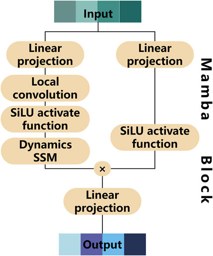
Figure 2. The structure of Mamba block, including linear projection layers, local convolutional layers, dynamic SSM modules.

2.3.2 Parameters

In the presented method, the Mamba model architecture is elegantly constructed with five meticulously stacked Mamba blocks, each configured with a state size of 64. This state size masterfully balances the dual imperatives of capturing ample information and maintaining computational efficiency, while also adeptly mitigating the peril of overfitting. Each block is designed to process sequences of length 100, a number meticulously selected to ensure that the model can adeptly process and learn from the intricate temporal dynamics embedded within the input data.

The batch size is thoughtfully set to 128, achieving an optimal equilibrium between memory utilization and training velocity. For the activation function, the Mamba model adopts the SiLU function, a function that stands apart from traditional activation functions by not saturating at either positive or negative extremes. This unique characteristic helps to preempt issues such as gradient vanishing or exploding, thereby ensuring a stable and efficient training process.

The model employs mean squared error (MSE) as its loss function, a choice that is ideally suited for pore pressure prediction tasks and provides a precise and unambiguous measure of the model’s prediction accuracy. For optimization, the model leverages the ADAM (Adaptive Moment Estimation) algorithm. By adaptively adjusting the learning rate for each parameter during training, ADAM facilitates faster convergence and superior performance.

During the training phase, Mamba leverages a convolutional mode to swiftly process the entire input sequence in a single pass. Conversely, during the inference phase, it adopts a recursive mode to incrementally process the input, allowing for incremental updates. This innovative architecture harnesses the efficient parallel processing capabilities of CNNs while preserving the adaptability of RNNs in managing sequence data, thereby ensuring optimal performance and flexibility.

3 Examples and results

Initially, we subjected our method to rigorous testing using a dataset derived from a work area in China, which comprised five wells. Wells A, B, and C, with a substantial 6,429 samples, served as the training data. Wells D and E, containing 4,103 samples, functioned as the test wells to evaluate the performance of the proposed method.

3.1 Well data test

Figures 3–5 display the logging curves of the training test wells, represented by green lines. Subfigures a to c illustrate the elastic attributes, including P-wave and S-wave velocities, and density, combining with time served as inputs for Mamba. It is noteworthy that pore pressure maintains a close correlation with depth. Considering that seismic data reside in the time domain, the transition from this domain to the depth domain is profoundly impacted by the velocity model. Logging data times can be conveniently deduced from the time-depth relationship, making time-depth a pivotal input attribute in our method. Subfigure d highlights the predictive targets, i.e., the pore pressure. The green line in this subfigure indicates the pore pressure curves, providing a visual benchmark for evaluating the predictions. These curves are provided by the engineers, which are extrapolated and refined based on the actual measurement points of formation pore pressure, as indicated by the pentahedrons in these figures. Furthermore, engineers extrapolate the formation pressure curve based on existing data and then refine it through actual drilling conditions (Ahmed A. et al., 2019; Abdelaal et al., 2022). The magenta color represents the prediction results. For clarity in these figures, we have thinned out the depth of the data.

Figure 3

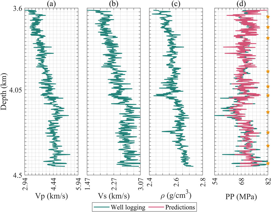
Figure 3. Logging curve and prediction results of training well A, (a) P-wave velocity; (b) S-wave velocity; (c) Density; (d) Formation pressure, where green represents logging values and magenta represents predicted values. The pentagram represents the position of the measured point.

Figure 4

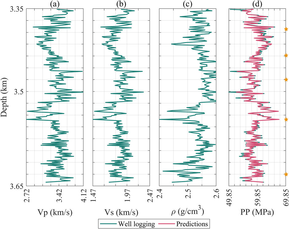
Figure 4. Logging curve and prediction results of training well B, (a) P-wave velocity; (b) S-wave velocity; (c) Density; (d) Formation pressure, where green represents logging values and magenta represents predicted values. The pentagram represents the position of the measured point.

Figure 5

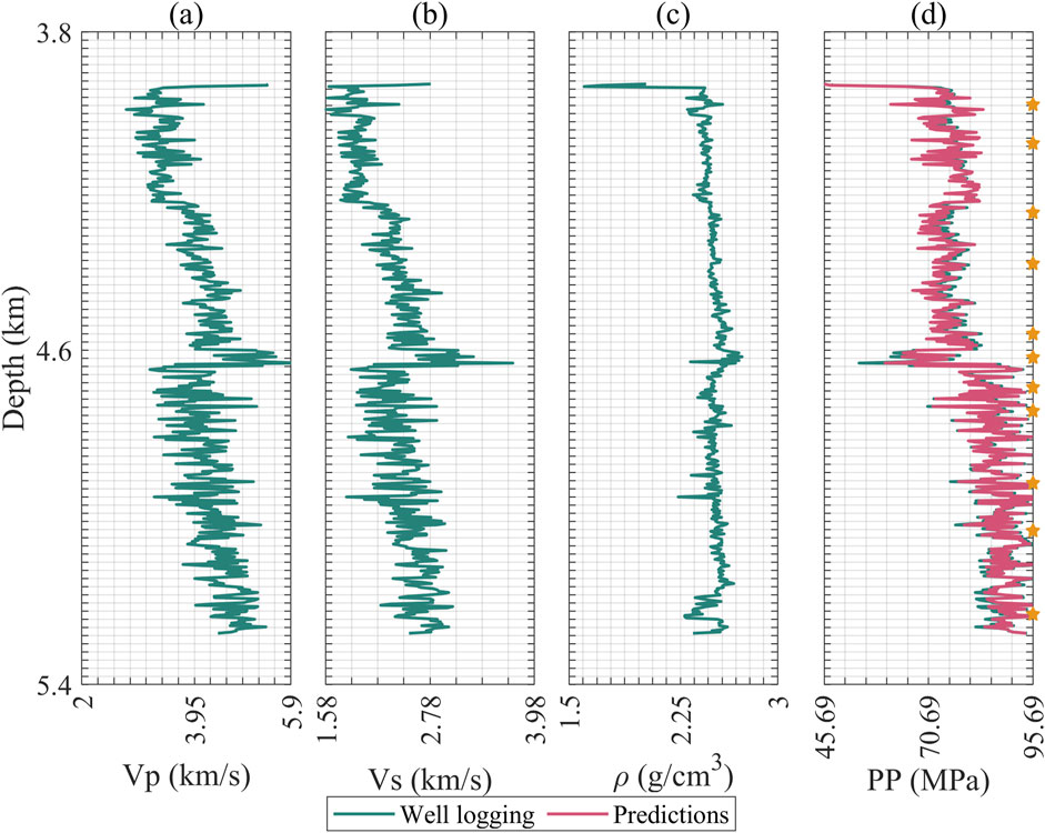
Figure 5. Logging curve and prediction results of training well C, (a) P-wave velocity; (b) S-wave velocity; (c) Density; (d) Formation pressure, where green represents logging values and magenta represents predicted values. The pentagram represents the position of the measured point.

Figure 6 provides the joint distribution plots. The histograms show that these input features have varying distribution characteristics, exhibiting irregular shapes. The complex nonlinear relationship between the input features and pore pressure poses significant challenges for estimation.

Figure 6

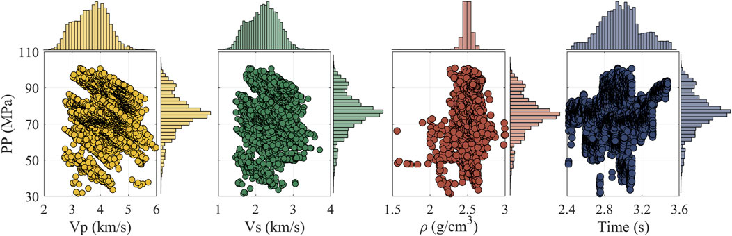
Figure 6. The joint distribution map. In the center of each subfigure is a cross plot that illustrates the relationship between pore pressure and different parameters. The top and right sides of each subfigure display the marginal distributions of the corresponding parameters and pore pressure. The intricate relationships depicted reveal that pore pressure does not adhere to a singular trend in relation to these parameters, thereby posing a significant challenge for accurate pore pressure prediction.

To further elaborate, for predicting pore pressure, the initial set of features comprises time depth, density, P-wave velocity, and S-wave velocity, resulting in an input feature matrix of size N$\times$ 4. Selecting appropriate hyperparameters for deep learning models is a delicate process that often relies heavily on human expertise and iterative testing (Krogh and Hertz, 1991; Smith, 2017; Smith, 2018). Given these considerations, we meticulously fine-tuned the hyperparameters of our Mamba model through a series of iterative trials. This included adjusting the state size and the sequence length to achieve optimal performance. Finally, in our example, the state size is set to 64 and the sequence length is set to 120 to develop a robust Mamba model tailored to our specific prediction tasks. During the training process, training data and validation data were randomly selected from three training wells in a ratio of 8:2. The predicted result of training wells is represented by the magenta line in subfigure d. As for the training well, the predicted results align closely with the trend of the pore pressure curve, demonstrating a high degree of agreement. At the measured points, the predicted values match excellently with the actual measurements.

Subsequently, we applied the trained model to the test data. Figures 7, 8 display the input attributes (excluding time depth) and the predicted property (highlighted in magenta line) for test wells. Visibly, the results closely match the actual measurements, validating the effectiveness of our approach. We also provide quantitative analysis by several metrics, including mean absolute deviation (MAD), mean absolute percent error (MAPE), root mean square error (RMSE), and the coefficient of determination(R²). These metrics measure the alignment between predicted and true values.

Figure 7

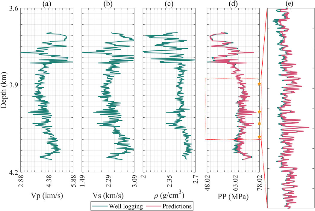
Figure 7. Logging curve and prediction results of blind test well D, (a) P-wave velocity; (b) S-wave velocity; (c) Density; (d) Formation pressure; (e) Measured pressure section enlargement, where green represents logging values and magenta represents predicted values. There are four measured points whose positions are indicated by pentagrams.

Figure 8

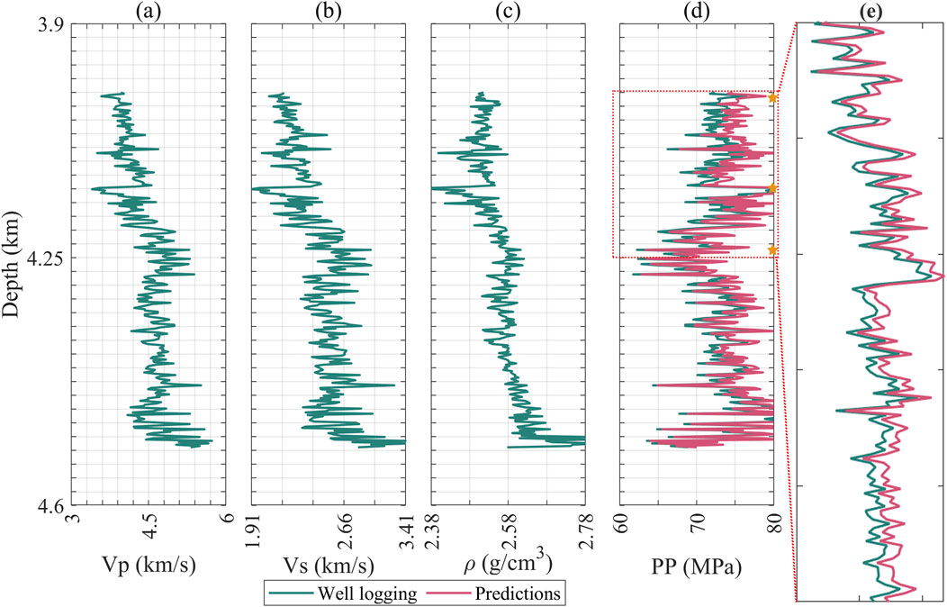
Figure 8. Logging curve and prediction results of blind test well E, (a) P-wave velocity; (b) S-wave velocity; (c) Density; (d) Formation pressure; (e) Measured pressure section enlargement, where green represents logging values and magenta represents predicted values. There are three measured points whose positions are indicated by pentagrams.

Figure 9a displays the convergence curve, with the blue line depicting training loss reduction per epoch. The orange line shows validation loss, assessing the performance of the model on unseen data. Lower loss values indicate better performance. Initially, both lines rapidly decline, signifying swift feature learning through parameter updates. As epochs increase, both training (blue) and validation (orange) losses stabilize, suggesting optimal weights and diminishing returns from further training. The smooth convergence curve without significant jitter indicates model stability. The gradual loss decline hints at smooth optimization and appropriate hyperparameters. The consistency of both lines in later epochs, without a spike in validation loss, implies good generalization, avoiding overfitting. This demonstrates the robustness of the method on training data and good predictive power on unknown data. Figure 9b shows the cross-plot between the actual measured value and predicted value. Clearly, the predicted results and measured data are evenly distributed on both sides of the diagonal, indicating good consistency between the predicted results and measured data. Figure 9c displays five violin plots, each corresponding to a different drill hole, with distinct colors representing the error data for each well. The white dot positioned at the center of each violin plot signifies the median of the error data, while the areas on both sides depict the probability density distribution of the data points. Overall, the prediction errors are centered around zero. Wells A and D exhibit broader violin shapes, indicating higher variability in their error data, especially prominent in Well A. Conversely, the error distributions for Wells B and E are more focused, with Well E displaying the narrowest range of data distribution, suggesting a more stable and consistent error profile. Well C distinguishes itself due to a notable outlier, which may indicate a significant discrepancy in its predictions. The tightly clustered and narrow distributions of errors in Wells B and E suggest superior prediction performance with minimal variability. These observations underscore the varying levels of reliability and accuracy across the wells, offering valuable insights into the predictive models employed for each.

Figure 9

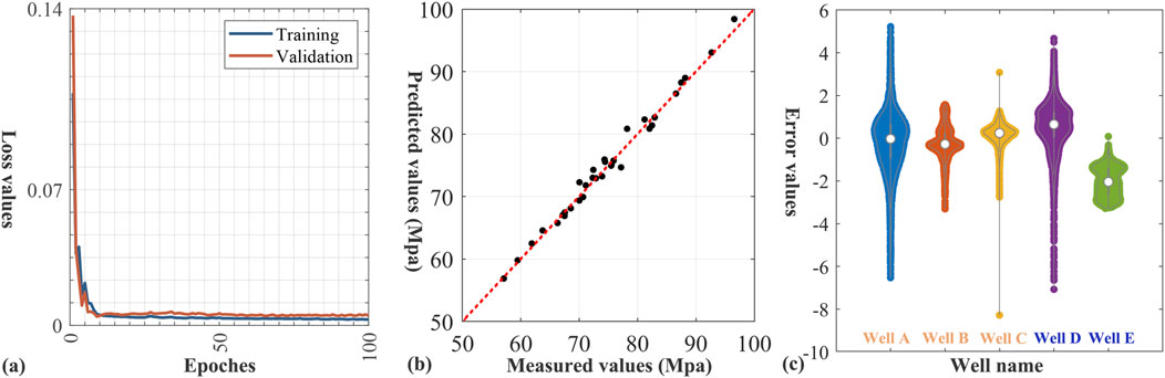
Figure 9. (a) Loss function. The blue and orange lines represent the training loss and validation loss, respectively. (b) Cross-plot between the actual measured value and predicted value at the points indicated by pentagrams in Figures 3–5, 7, 8. (c) Violin plots of errors between logging curves and predictions from different wells. The wells marked in the orange font are training wells, while the ones in the blue are testing wells.

Table 1 presents the precision results of different wells. Generally, lower mean absolute percentage error (MAPE), and mean square error (MSE) values indicate a better model fit, while a higher Pearson correlation coefficient (R) value signifies a closer alignment between predictions and true values. The small value of median absolute deviation (MAD) means that the prediction error is relatively concentrated. From the table, it is evident that both the training and testing well prediction results demonstrate minimal errors and exhibit strong correlations with the pore pressure curve, confirming the feasibility and reliability of the method.

Table 1

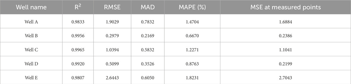
Table 1. Quantitative analysis of prediction error in different wells. The wells marked in orange font are training wells, while the ones in blue are testing wells.

3.2 Seismic data application

The ultimate aim of this work is to acquire 3D volumes of estimated pore pressure. After validating our proposed method on individual wells, we broaden its application to seismic data. All wells are incorporated into the training process for predicting pore pressure in seismic data area, adhering to the same training procedures. The network architecture and hyperparameters remain identical to those utilized in the well-based example.

Initially, we train a model that is then applied to seismic data. The 3D volumes of density, P- and S-wave velocity are derived from pre-stack seismic inversion technologies (Liu et al., 2020; Zhou et al., 2022; Shi et al., 2023; Sun et al., 2024. For clarity, Figure 10 shows two seismic sections along Inline and Xline directions that are randomly extracted from the 3D seismic volumes. The corresponding 2D sections of density, P-wave, and S-wave velocities are exhibited in Figure 11, respectively. These three elastic attributes and time volumes are input into the optimized Mamba model. The predicted volumes of pore pressure are illustrated in Figure 12.

Figure 10

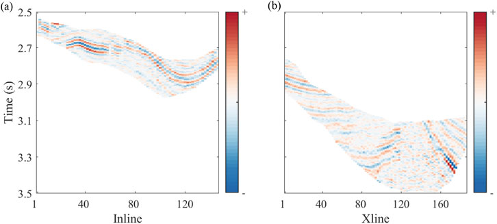
Figure 10. Two seismic sections randomly extracted along different directions.

Figure 11

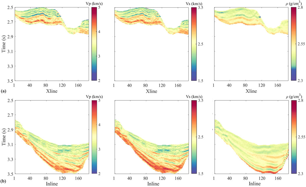
Figure 11. Sections of elastic attributes corresponding the seismic section in Figure 10, respectively, which combine with the time section as input attributes.

Figure 12

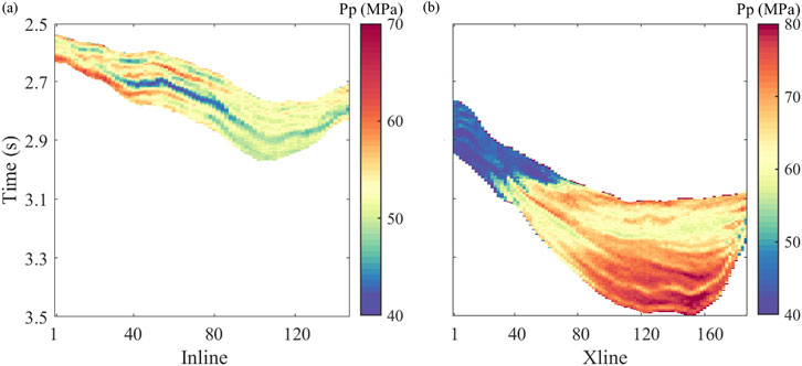
Figure 12. 2D pore pressure section corresponding to the seismic section in Figure 10 that are predicted by using the Mamba model.

These predictions not only reflect the intricate formation structure but also meticulously delineate the three-dimensional spatial configuration of pore pressure. It is noteworthy that, despite refraining from employing rock physics modeling to bolster our training samples, the predictions retained a commendable degree of rationality and satisfaction. Observing the seismic profile, shallow pore pressures reveal layered attributes, with relatively consistent formation pressure values within each layer, hinting that lithology plays a pivotal role in governing pore pressure at these depths. However, as the depth (or time) increases, the pore pressure in subterranean sections undergoes a notable surge, as vividly depicted in Figure 12B. This suggests that depth transcends the solitary influence of lithology, exerting a broader and more profound impact.

Figure 13 shows the formation pore pressure slice of the target interval, and it can be seen from the figure that the pore pressure in the studied area presents a significant differential distribution. In the presented figure, the hue of red denotes a region of relatively high pore pressure, whereas blue symbolizes areas of comparatively low pore pressure. Additionally, yellow serves to mark those zones exhibiting moderate pore pressure values. The concentration of red hues is particularly evident in the southeastern vicinity of the fault, suggesting an accumulation of high pore pressure on that specific side. Conversely, the yellow-colored areas, which represent moderate pore pressure, are positioned to the northwest of the fault, reflecting a state of relatively stable median pore pressure in that region. Adjacent to the fault, there is a noticeable abrupt decrease in pore pressure, resulting in zones characterized by lower values. The successful implementation of this method highlights its potential for quantitatively evaluating the spatial distribution of pore pressure.

Figure 13

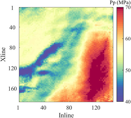
Figure 13. The slice of the predicted pore pressure at the target layer. The spatial distribution characteristics of pore pressure can be clearly seen from the figure.

4 Discussion

Through the implementation of our proposed method, leveraging a fundamental Mamba network, we achieved a relatively accurate prediction of 3D pore pressure. Our primary objective was to establish a viable and reliable approach for predicting the spatial distribution of pore pressure. The results obtained validate the feasibility of this method and demonstrate that the model can be generalized for broader application.

In our experiments, all the parameters related to the Mamba model are obtained through trial and error, and the method of automatically determining these parameters needs further research. In essence, the configuration of Mamba for pore pressure prediction is meticulously fine-tuned to strike a balance between computational efficiency, model capacity, and training stability, rendering it a resilient and versatile choice for a wide array of complex tasks.

It is worth noting that we did not directly compare our method with other existing pore pressure prediction techniques, as most of these methods are primarily focused on one-dimensional predictions and have not been adapted for three-dimensional applications. However, the successful deployment of our method underscores its potential for providing quantitative evaluations of three-dimensional pore pressure.

Seismic data serve as the primary source of reservoir information in the inter-well space, primarily comprising elastic properties derived from seismic inversion. However, wells offer a diverse array of inputs, suggesting that elastic parameters may not necessarily be the sole or primary inputs for pore pressure prediction. For instance, the correlation between porosity and pore pressure could also be considered. To further refine the accuracy of our predictions, we propose incorporating additional logging curves and drilling performance data into the estimation process. This holistic approach can significantly enhance our ability to predict pore pressure with greater precision and reliability.

5 Conclusion

We successfully established an efficient and precise the spatial distribution of formation pressure prediction system by integrating deep learning technology with seismic inversion methods. The model fully leverages the spatial continuity of seismic data, effectively tackling the prediction challenges posed by geological complexity, and significantly boosting the accuracy and reliability of three-dimensional formation pressure predictions. Specifically, pore pressure prediction has transcended one-dimensional limitations, achieving true three-dimensional visualization, thereby furnishing more comprehensive and detailed geological information for decision-making in oil and gas exploration and development. Furthermore, the incorporation of the Mamba model enhances the capacity to capture features from time-series data, such as well logging and seismic data. As a structured state-space sequence model, it combines hardware-aware algorithms and convolution acceleration mechanisms to recursively compute the model, drastically improving computational efficiency and enabling the effective capture of complex dependencies within sequential data. Examples of logging and seismic predictions illustrate that this method can attain high-precision spatial distribution of pore pressure prediction results, providing a scientific foundation for identifying potential high-pressure/low-pressure anomalies, predicting formation fracture risks, and optimizing drilling paths.

Data availability statement

The datasets presented in this article are not readily available because the data used in this study is confidential and shall not be disclosed to any third party without prior authorization. Requests to access the datasets should be directed to Bing Liu, MjUyOTcyMDgzMkBxcS5jb20=.

Author contributions

Xingye Liu: Conceptualization, Funding acquisition, Methodology, Writing–original draft, Writing–review and editing. Bing Liu: Methodology, Writing–original draft, Writing–review and editing. Wenyue Wu: Writing–original draft, Writing–review and editing. Qian Wang: Methodology, Writing–review and editing. Yuwei Liu: Data curation, Formal Analysis, Writing–review and editing.

Funding

The author(s) declare that financial support was received for the research and/or publication of this article. This work is supported by the Open Fund of “Study on in-situ stress prediction method for terrestrial shale oil reservoirs driven by knowledge and data” from the National Energy Shale Oil Research and Development Center under Grant 33550000-24-ZC0613-0049, the Sinopec Science and Technology Department Key Project: “Research on Formation Pressure and In-situ stress Prediction Technology of Continental Shale Oil Reservoirs” under Grant P24078, and Sichuan Science and Technology Program under Grant 2024NSFSC1984 and Grant 2024NSFSC1990. The authors declare that this study received funding from Sinopec. The funder was not involved in the study design, collection, analysis, interpretation of data, the writing of this article, or the decision to submit it for publication.

Conflict of interest

Author WW was employed by Sichuan Water Development Investigation, Design Research Co., Ltd.

Author YL was employed by SinoPEC Petroleum Exploration and Production Research Institute.

The remaining authors declare that the research was conducted in the absence of any commercial or financial relationships that could be construed as a potential conflict of interest.

Generative AI statement

The authors declare that no Generative AI was used in the creation of this manuscript.

Publisher’s note

All claims expressed in this article are solely those of the authors and do not necessarily represent those of their affiliated organizations, or those of the publisher, the editors and the reviewers. Any product that may be evaluated in this article, or claim that may be made by its manufacturer, is not guaranteed or endorsed by the publisher.

Supplementary material

The Supplementary Material for this article can be found online at: https://www.frontiersin.org/articles/10.3389/feart.2025.1530557/full#supplementary-material

References

Abdelaal, A., Elkatatny, S., and Abdulraheem, A. (2022). Real-time prediction of formation pressure gradient while drilling. Sci. Rep. 12, 11318. doi:10.1038/s41598-022-15493-z

PubMed Abstract | CrossRef Full Text | Google Scholar

Ahmed, A., Elkatatny, S., Ali, A., Mahmoud, M., and Abdulraheem, A. (2019a). New model for pore pressure prediction while drilling using artificial neural networks. Arabian J. Sci. Eng. 44, 6079–6088. doi:10.1007/s13369-018-3574-7

CrossRef Full Text | Google Scholar

Ahmed, N., Waldemar Weibull, W., Grana, D., and Bhakta, T. (2024a). Constrained nonlinear amplitude-variation-with-offset inversion for reservoir dynamic changes estimation from time-lapse seismic data. Geophysics 89, R1–R15. doi:10.1190/geo2022-0750.1

CrossRef Full Text | Google Scholar

Ahmed, N., Weibull, W., Bhakta, T., and Luo, X. (2024b). “Viscoelastic seismic inversion for time-lapse saturation and pore pressure changes monitoring,” in 85th EAGE Annual Conference and Exhibition (including the Workshop Programme) (Houten, Netherlands European Association of Geoscientists and Engineers), 1–5. doi:10.3997/2214-4609.2024101684

CrossRef Full Text | Google Scholar

Ahmed, S. A., Mahmoud, A. A., Elkatatny, S., Mahmoud, M., and Abdulraheem, A. (2019b). “Prediction of pore and fracture pressures using support vector machine,” in International petroleum technology conference (IPTC). doi:10.2523/IPTC-19523-MS

CrossRef Full Text | Google Scholar

Aliouane, L., Ouadfeul, S.-A., and Boudella, A. (2015). “Pore pressure prediction in shale gas reservoirs using neural network and fuzzy logic with an application to barnett shale,” in EGU General Assembly Conference.

Google Scholar

Andrian, D., Rosid, M., and Septyandy, M. (2020). Pore pressure prediction using anfis method on well and seismic data field “ayah”. IOP Conf. Ser. Mater. Sci. Eng. 854, 012041. doi:10.1088/1757-899X/854/1/012041

CrossRef Full Text | Google Scholar

Cao, S., Wang, C., Niu, Q., Zheng, Q., Shen, G., Chen, B., et al. (2024). Enhancing pore pressure prediction accuracy: a knowledge-driven approach with temporal fusion transformer. Geoenergy Sci. Eng. 238, 212839. doi:10.1016/j.geoen.2024.212839

CrossRef Full Text | Google Scholar

Chopra, S., and Huffman, A. R. (2006). Velocity determination for pore-pressure prediction. Lead. Edge 25, 1502–1515. doi:10.1190/1.2405336

CrossRef Full Text | Google Scholar

Dao, T., and Gu, A. (2024). “Transformers are SSMs: generalized models and efficient algorithms through structured state space duality,” in International Conference on Machine Learning (ICML). doi:10.48550/arXiv.2405.21060

CrossRef Full Text | Google Scholar

Farsi, M., Mohamadian, N., Ghorbani, H., Wood, D. A., Davoodi, S., Moghadasi, J., et al. (2021). Predicting formation pore-pressure from well-log data with hybrid machine-learning optimization algorithms. Nat. Resour. Res. 30, 3455–3481. doi:10.1007/s11053-021-09852-2

CrossRef Full Text | Google Scholar

Gedon, D., Wahlström, N., Schön, T. B., and Ljung, L. (2020). “Deep state space models for nonlinear system identification,” in 19th IFAC Symposium on System Identification (SYSID). doi:10.1016/j.ifacol.2021.08.406

CrossRef Full Text | Google Scholar

Greenwood, J., Russell, R., and Dautel, M. (2009). “The use of lwd data for the prediction and determination of formation pore pressure,” in SPE Asia Pacific Oil and Gas Conference and Exhibition (Dallas, United States: SPE). doi:10.2118/124012-MS

CrossRef Full Text | Google Scholar

Gu, A., and Dao, T. (2023). Mamba: linear-time sequence modeling with selective state spaces. arXiv preprint arXiv:2312.00752. doi:10.48550/arXiv.2312.00752

CrossRef Full Text | Google Scholar

Gu, A., Goel, K., and Ré, C. (2021). Efficiently modeling long sequences with structured state spaces. arXiv preprint arXiv:2111.00396. doi:10.48550/arXiv.2111.00396

CrossRef Full Text | Google Scholar

Hadi, F., Eckert, A., and Almahdawi, F. (2019). “Real-time pore pressure prediction in depleted reservoirs using regression analysis and artificial neural networks,” in SPE Middle East Oil and Gas Show and Conference (Dallas, United States: SPE). doi:10.2118/194851-MS

CrossRef Full Text | Google Scholar

Haris, A., Sitorus, R., and Riyanto, A. (2017). Pore pressure prediction using probabilistic neural network: case study of south sumatra basin. IOP Conf. Ser. Earth Environ. Sci. 62, 012021. doi:10.1088/1755-1315/62/1/012021

CrossRef Full Text | Google Scholar

Hazra, B., Chandra, D., and Vishal, V. (2024). “Upscaling for natural gas estimates in coal and shale,” in Unconventional hydrocarbon reservoirs: coal and shale (Springer), 101–123. doi:10.1007/978-3-031-53484-3_5

CrossRef Full Text | Google Scholar

Hochreiter, S., and Schmidhuber, J. (1997). Long short-term memory. Neural Comput. 9, 1735–1780. doi:10.1162/neco.1997.9.8.1735

PubMed Abstract | CrossRef Full Text | Google Scholar

Huang, H., Li, J., Yang, H., Wang, B., Gao, R., Luo, M., et al. (2022). Research on prediction methods of formation pore pressure based on machine learning. Energy Sci. and Eng. 10, 1886–1901. doi:10.1002/ese3.1112

CrossRef Full Text | Google Scholar

Hussain, M., and Ahmed, N. (2018). Reservoir geomechanics parameters estimation using well logs and seismic reflection data: insight from sinjhoro field, lower indus basin, Pakistan. Arabian J. Sci. Eng. 43, 3699–3715. doi:10.1007/s13369-017-3029-6

CrossRef Full Text | Google Scholar

Hutomo, P., Rosid, M., and Haidar, M. (2019). Pore pressure prediction using eaton and neural network method in carbonate field “x” based on seismic data. IOP Conf. Ser. Mater. Sci. Eng. 546, 032017. doi:10.1088/1757-899X/546/3/032017

CrossRef Full Text | Google Scholar

Keshavarzi, R., and Jahanbakhshi, R. (2013). Real-time prediction of pore pressure gradient through an artificial intelligence approach: a case study from one of middle east oil fields. Eur. J. Environ. Civ. Eng. 17, 675–686. doi:10.1080/19648189.2013.811614

CrossRef Full Text | Google Scholar

Krishna, S., Irfan, S. A., Keshavarz, S., Thonhauser, G., and Ilyas, S. U. (2024). “Smart predictions of petrophysical formation pore pressure via robust data-driven intelligent models,” in Multiscale and multidisciplinary modeling, experiments and design, 1–20. doi:10.1007/s41939-024-00542-z

CrossRef Full Text | Google Scholar

Krogh, A., and Hertz, J. (1991). A simple weight decay can improve generalization. Adv. Neural Inf. Process. Syst. 4, 951–957.

Google Scholar

LeCun, Y., Bottou, L., Bengio, Y., and Haffner, P. (1998). Gradient-based learning applied to document recognition. Proc. IEEE 86, 2278–2324. doi:10.1109/5.726791

CrossRef Full Text | Google Scholar

Liu, X., Chen, X., Li, J., Zhou, X., and Chen, Y. (2020). Facies identification based on multikernel relevance vector machine. IEEE Trans. Geoscience Remote Sens. 58, 7269–7282. doi:10.1109/TGRS.2020.2981687

CrossRef Full Text | Google Scholar

Liu, X., Zhou, H., Guo, K., Li, C., Zu, S., and Wu, L. (2023). Quantitative characterization of shale gas reservoir properties based on bilstm with attention mechanism. Geosci. Front. 14, 101567. doi:10.1016/j.gsf.2023.101567

CrossRef Full Text | Google Scholar

MacBeth, C. (2004). A classification for the pressure-sensitivity properties of a sandstone rock frame. Geophysics 69, 497–510. doi:10.1190/1.1707070

CrossRef Full Text | Google Scholar

Mylnikov, D., Nazdrachev, V., Korelskiy, E., Petrakov, Y., and Sobolev, A. (2021). “Artificial neural network as a method for pore pressure prediction throughout the field,” in SPE Russian Petroleum Technology Conference? (Dallas, United States: SPE). doi:10.2118/206558-MS

CrossRef Full Text | Google Scholar

Naeini, E. Z., Green, S., Russell-Hughes, I., and Rauch-Davies, M. (2019). An integrated deep learning solution for petrophysics, pore pressure, and geomechanics property prediction. Lead. Edge 38, 53–59. doi:10.1190/tle38010053.1

CrossRef Full Text | Google Scholar

Pham, T., Zhang, L., and Chen, J. (2020). Application of cnn and lstm networks for logging data interpretation. J. Geophys. Eng. doi:10.1093/jge/xyz123

CrossRef Full Text | Google Scholar

Qi, H., Yang, S., Hu, S., Kong, D., Xu, F., Jiang, X., et al. (2024). Back propagation neural network model for controlling artificial rocks petrophysical properties during manufacturing process. Petroleum Sci. Technol., 1–27. doi:10.1080/10916466.2024.2415520

CrossRef Full Text | Google Scholar

Radwan, A. E., Wood, D. A., and Radwan, A. A. (2022). Machine learning and data-driven prediction of pore pressure from geophysical logs: a case study for the mangahewa gas field, New Zealand. J. Rock Mech. Geotechnical Eng. 14, 1799–1809. doi:10.1016/j.jrmge.2022.01.012

CrossRef Full Text | Google Scholar

Sanei, M., Ramezanzadeh, A., and Delavar, M. R. (2023). Applied machine learning-based models for predicting the geomechanical parameters using logging data. J. Petroleum Explor. Prod. Technol. 13, 2363–2385. doi:10.1007/s13202-023-01687-2

CrossRef Full Text | Google Scholar

Shi, S., Qi, Y., Chang, W., Li, L., Yao, X., and Shi, J. (2023). Acoustic impedance inversion in coal strata using the priori constraint-based tcn-bigru method. Adv. Geo-Energy Res. 9, 13–24. doi:10.46690/ager.2023.07.03

CrossRef Full Text | Google Scholar

Smith, L. N. (2017). “Cyclical learning rates for training neural networks,” in 2017 IEEE winter conference on applications of computer vision (WACV), 464–472. doi:10.1109/WACV.2017.58

CrossRef Full Text | Google Scholar

Smith, L. N. (2018). A disciplined approach to neural network hyper-parameters: Part 1–learning rate, batch size, momentum, and weight decay. arXiv preprint arXiv:1803.09820. doi:10.48550/arXiv.1803.09820

CrossRef Full Text | Google Scholar

Soares, A., Nunes, R., Salvadoretti, P., Costa, J. F., Martins, T., Santos, M., et al. (2024). Pore pressure uncertainty characterization coupling machine learning and geostatistical modelling. Math. Geosci. 56, 691–709. doi:10.1007/s11004-023-10102-9

CrossRef Full Text | Google Scholar

Sun, H., Zhang, J., Xue, Y., and Zhao, X. (2024). Seismic inversion based on fusion neural network for the joint estimation of acoustic impedance and porosity. IEEE Trans. Geoscience Remote Sens. 62, 1–10. doi:10.1109/TGRS.2024.3426563

CrossRef Full Text | Google Scholar

Syed, F. I., AlShamsi, A., Dahaghi, A. K., and Neghabhan, S. (2022). Application of ml and ai to model petrophysical and geomechanical properties of shale reservoirs–a systematic literature review. Petroleum 8, 158–166. doi:10.1016/j.petlm.2020.12.001

CrossRef Full Text | Google Scholar

Voelker, A. R., and Eliasmith, C. (2018). Improving spiking dynamical networks: accurate delays, higher-order synapses, and time cells. Neural Comput. 30, 569–609. doi:10.1162/neco_a_01046

PubMed Abstract | CrossRef Full Text | Google Scholar

Yilmaz, O. (2001). Seismic data analysis: processing, inversion, and interpretation of seismic data. Tulsa, OK: Society of Exploration Geophysicists. doi:10.1190/1.9781560801580

CrossRef Full Text | Google Scholar

Yu, C., Ljung, L., and Verhaegen, M. (2018). Identification of structured state-space models. Automatica 90, 54–61. doi:10.1016/j.automatica.2017.12.023

CrossRef Full Text | Google Scholar

Zhang, G., Davoodi, S., Band, S. S., Ghorbani, H., Mosavi, A., and Moslehpour, M. (2022). A robust approach to pore pressure prediction applying petrophysical log data aided by machine learning techniques. Energy Rep. 8, 2233–2247. doi:10.1016/j.egyr.2022.01.012

CrossRef Full Text | Google Scholar

Zhang, X., Lu, Y.-H., Jin, Y., Chen, M., and Zhou, B. (2024). An adaptive physics-informed deep learning method for pore pressure prediction using seismic data. Petroleum Sci. 21, 885–902. doi:10.1016/j.petsci.2023.11.006

CrossRef Full Text | Google Scholar

Zhou, L., Li, J., Yuan, C., Liao, J., Chen, X., Liu, Y., et al. (2022). Bayesian deterministic inversion based on the exact reflection coefficients equations of transversely isotropic media with a vertical symmetry axis. IEEE Trans. Geoscience Remote Sens. 60, 1–15. doi:10.1109/TGRS.2022.3176628

CrossRef Full Text | Google Scholar

Zong, Z., Zhang, J., and Chen, F. (2024). Seismic prediction for formation pressure considering diagenesis effect. IEEE Trans. Geoscience Remote Sens. 62, 1–13. doi:10.1109/TGRS.2024.3428616

CrossRef Full Text | Google Scholar