A machine learning model for the prediction of hail-affected area in Germany

Hailstorms pose significant risks in Germany, calling for accurate forecasts and warnings. This study explores the application of a convolutional neural network (CNN) to predict daily hail-affected areas using radar-based hail footprints from 2005 to 2019. The ML model utilizes 18 thermodynamic and dynamic convection-related parameters derived from ERA5 reanalysis data. Feature selection identifies seven key predictors, with a particular emphasis on the convective available potential energy and bulk wind shear (CAPESHEAR). Model performance is assessed against climatology- and persistence-based reference forecasts, and sensitivity analyses using gradient-weighted class activation mapping (Grad-CAM) are conducted to interpret the predictions. The CNN model significantly outperforms the reference forecasts, achieving a Heidke Skill Score (HSS) of up to 0.66 for large hail-affected areas. However, lower predictive skill is observed on days with weak CAPESHEAR values or when hailstorms are isolated. Sensitivity analysis highlights CAPESHEAR as the dominant predictor influencing model decisions. These findings demonstrate the potential of ML-based hail prediction using only convective environmental parameters. Given its low computational demand once trained, this approach offers a promising tool for operational forecasting. It would be desirable to extend this approach to a more regional perspective and to include information on severity.

1 Introduction

Severe convective storms (SCSs) can create various types of hazardous weather, including hail, wind gusts, tornadoes, and heavy precipitation. Hail, in particular, can cause significant damage to buildings, infrastructure, and agriculture. Both economic and insured losses have substantially increased over recent years globally, with the highest increase in Europe. For example, the insured losses in Germany caused mainly by hail during two recent SCS series on 27/28 July 2013 and 10 June 2019 (Kunz et al., 2018; Wilhelm et al., 2021) sum up to €2.7 bn and €0.75 bn, respectively (MunichRE, 2020). Comprehensive understanding of the favorable environmental conditions for hailstorms is crucial to improve the accuracy of hail predictions, facilitating timely and effective preventive actions to be taken.

There are two main challenges in improving hail forecasts based on numerical weather prediction (NWP) models. First, the development of hail-producing SCSs involves complex interactions of various dynamic and thermodynamic processes on a broad range of spatial and temporal scales (e.g., frontal circulations, atmospheric convection, cloud microphysics) (Markowski and Richardson, 2011). The representation of the underlying non-linear dynamics and scale-interactions in NWP models is a challenge, as the relevant triggering and intensification mechanisms for SCSs are not fully resolved by the observations assimilated into the NWP models. Further, the related cloud microphysics exhibit high complexity and are highly sensitive to parameter variations (Wellmann et al., 2020). Also, the prediction of hail requires two- or even three-moment cloud microphysics parameterization schemes for mixed-phase clouds (e.g., Seifert and Beheng, 2006; Khain et al., 2015), which are computationally too expensive to be used in operational NWP or climate models.

Therefore, several studies rely on so-called ingredient-based predictions using a combination of convection-related ambient conditions as proxies that are derived from NWP data (Trapp et al., 2011; Malečić et al., 2022; Torralba et al., 2023). On the large-scale, parameters include the synoptic flow pattern, atmospheric teleconnections, or different weather regimes (Aran et al., 2011; Piper and Kunz, 2017; Kunz et al., 2020). With regard to the prediction of hail, it has been noted that severe hailstorms, producing hailstones with a diameter of at least 2 cm, typically develop in conditions characterized by high levels of convective available potential energy (CAPE) and 0–6 $\mathrm{k}\mathrm{m}$ bulk wind shear (BULKSH). CAPE is directly linked to the strength of updrafts, while vertical wind shear is decisive for the organization and structure of the convective systems, such as single cells, multicells, supercells, and mesoscale convective systems (Markowski and Richardson, 2011; Púčik et al., 2015). Wind shear also determines the residence time of the hail embryos in the updraft, and thus indirectly determines the maximum size of the hailstones (Kumjian and Lombardo, 2020; Kumjian et al., 2021). Studies have also revealed that deep-layer shear (DLS) and storm-relative helicity (SRH) significantly influence the life cycle of SCSs, with long-lasting events occurring exclusively under high SRH conditions (Kunz et al., 2018; 2020; Wilhelm et al., 2023; Tonn et al., 2023).

The second major obstacle in improving hail predictions is the lack of direct hail observations for evaluation purposes in Germany and most other countries - except of France, northern Italy, and Croatia, where high-density hailpad networks have been in operation over several decades (Dessens et al., 2015; Manzato et al., 2022). While geostationary satellites can indirectly detect potentially hail-producing storms by capturing the overshooting tops of cumulonimbus clouds (Punge and Kunz, 2016), they fall short in precisely monitoring actual hail occurrences beneath the clouds. Valuable information about (hail-producing) SCSs is provided by weather radars, despite several potential artifacts such as beam shielding and signal attenuation. In particular, weather radar networks as deployed in Germany by the German Weather Service (Deutscher Wetterdienst, DWD) enable the monitoring of thunderstorm propagation, the evolution of their intensity, vertical structure, and further properties because of their high spatial and temporal resolutions and the large area under permanent surveillance (Puskeiler et al., 2016; Wapler, 2017; Fluck et al., 2021).

In recent years, machine learning (ML) methods have been successfully adopted to assess or predict thunderstorm and hail occurrence by leveraging known relationships between hailstorms and ambient conditions (Gagne et al., 2015; 2017; Gagne et al., 2019; Czernecki et al., 2019; Pulukool et al., 2020; Leinonen et al., 2022; Auliya et al., 2023; Ackermann et al., 2023). The majority of ML models has focused on nowcasting to short-range forecasts, i.e., typical lead times ranging from 12 to 36 h (Gagne et al., 2019). This focus is mostly due to the significant challenge of forecasting convection initiation and occurrence at longer lead times without the support of NWP techniques (McGovern et al., 2023). In recent research, different ML models have been used to predict hail size or convective precipitation by taking related environmental conditions from reanalysis data or ensemble forecast in combination with data from remote sensing instruments, such as radar reflectivity (Gagne et al., 2017; Czernecki et al., 2019; Burke et al., 2020; Han et al., 2021; Leinonen et al., 2022; Ackermann et al., 2023). Gagne et al. (2019), for example, found that Convolutional Neural Networks (CNNs) exhibit superior predictive performance compared to other ML techniques for the prediction of hail events of at least 2.5 cm size based on numerical model outputs. The CNN also identified correlations between the likelihood of severe hail and convective environmental conditions. However, it is important to note that the ML models in their study were trained to predict hail sizes estimated from NWP model output rather than actual hail size observations. Despite challenges in applying ML techniques, such as a balanced data sample, which also needs to be large enough to be divided into a training and a validation period, the potential for ML applications in convection prediction is huge and development has only just begun.

The purpose of this paper is to train a deep learning model for deterministic predictions of the daily hail-affected area in Germany using a combination of ambient conditions. The ambient conditions are derived from gridded ERA5 reanalysis data (Hersbach et al., 2020) from the European Centre for Medium-Range Weather Forecasts (ECMWF). The hail-affected area is obtained from radar-identified hail tracks over Germany using the radar network from DWD (Puskeiler et al., 2016; Schmidberger, 2018). The study addresses the following specific research questions:

1. What is the skill of an ML-based model to predict the daily hail-affected area in Germany?

2. Which predictors contribute most to the model’s skill, and what is their relative importance within the ML model?

3. In which weather conditions does the ML model demonstrate the highest or lowest predictive skill, and what are the underlying reasons for this?

In Sections 2 and 3, we present detailed information about the data and methods employed, including the setup of the ML model. Following that, Sections 4–6 present the study’s results. Though Section 4 focuses on a statistical analysis of the hailstorm environment, Section 5 builds on this foundation by comprehensively evaluating the skill of the developed ML model. The insights obtained from this evaluation guide the meteorological interpretations in Section 6, specifically focusing on prediction errors. Section 7 summarizes the findings and gives some ideas for future research.

2 Data description

In this study, two different proxy datasets were used to establish a relationship between hail events and ambient condition: Tracks of potential hailstorms derived from 3D radar reflectivity (Sec. 2.1) and ERA5 reanalysis from ECMWF (Sec. 2.2). We consider only the summer half-year from April to September, when hail occurs most frequently in Germany and Central Europe (Kunz, 2007) for the 15-year period from 2005 to 2019. The study area extends from 44 to 56°N, and from 4 to 16°E, covering all of Germany.

2.1 Potential hailstorm tracks

Tracks of SCS are objectively obtained from the application of the radar-based cell detection and tracking algorithm TRACE3D (Handwerker, 2002). Though originally developed for spherical coordinates from a single radar, TRACE3D is applied here in a modified setup (Puskeiler et al., 2016) for 3D radar reflectivity on a Cartesian grid. We used the so-called PZ-product with six reflectivity classes (7, 19, 28, 37, 46, 55 dBZ) at twelve vertical levels from DWD’s C-band radar network with a temporal resolution of 15 min and a spatial resolution of 2 km. The reason for using the PZ product is the availability of data records since 2005.

TRACE3D essentially carries out two main steps: An initial reflectivity threshold is set to identify and mark areas of intense precipitation. Then, using a second threshold, it determines the highest reflectivity value within this region, referred to as “reflectivity core”. The second step involves linking these reflectivity cores with their counterparts from the radar scan before. To best identify potentially hail-producing cells, a lower threshold of 55 dBZ is considered, regardless of the height above ground (Puskeiler et al., 2016; Schmidberger, 2018). The tracking algorithm computes complete tracks of SCSs with a high likelihood of hail reaching the ground according to the evaluation with insurance loss data (Puskeiler et al., 2016). Because of the uncertainty inherent in both radar observations and the tracking algorithm, it cannot be assured that each radar-identified track was actually associated with hail on the ground. Therefore, the SCS tracks are hereafter referred to as “potential” hail track.

The data provided for this study include information on the geographical center point of the tracks, the average direction of motion $({\varphi }_{\mathit{obs}})$, velocity $(v_{\mathit{obs}})$, as well as length and width. Note that we only consider times when the reflectivity exceeds the 55 dBZ threshold (Tonn et al., 2023). The entire SCS’s life cycles can be considerably longer.

For the period 2005–2019, a total of 7,702 potential hail tracks are identified. To estimate the potentially hail-affected area for each track, we multiply the track’s length by its average width on the spherical surface of the Earth (Figure 1). The estimated length of the hail track is determined by the duration and moving direction and velocity of SCSs from the Trace3D algorithm. The average width is obtained by averaging the different width of detected radar reflectivity cores of at least 55 dBZ along the track. Our main focus is the daily aggregation of the potentially hail-affected area in Germany. This area, which is highly relevant for potential damages, serves as the target variable for our ML approach.

Figure 1

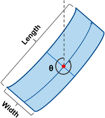
Figure 1. The polygon shows the area affected by a single hail streak on a curved Earth surface, and the red dot is the centre of the hailstorm at a certain time, $\theta$ shows the direction of the hail track.

2.2 ERA5 reanalysis

The ERA5 reanalysis provides hourly estimates of atmospheric, ocean, and land-surface variables. It is based on 4-dimensional variational analysis with the Integrated Forecasting System (IFS) Cy41r2 (Hersbach et al., 2020; ECMWF, 2023). In this study, ERA5 data are used on a regular latitude-longitude grid of $0.25\times 0.25$°horizontal grid spacing. At each grid cell, vertical profiles of pressure, temperature, specific humidity, wind speed and direction are used to derive thermodynamic, dynamic and stability parameters. The parameters for our study are taken at 12 UTC and 18 UTC as hailstorms occur most frequently during this time of the day in Germany (Kunz, 2007; Fluck et al., 2021) which is characterized by the maximum diurnal heating. In our investigation, we primarily rely on the $12\mathrm{U}\mathrm{T}\mathrm{C}$ ERA5 fields as this point in time best characterizes the convective environment prior to most hailstorm developments on the same day.

3 Methodology

3.1 Selection of convective parameters

To include as much useful information about convective environments as possible and to reduce the risk of overfitting, our selection of variables accounts for correlations between different convective parameters identified in the study of Wilhelm et al. (2023). They found, for example, that dynamic parameter largely co-vary (e.g., wind shear, storm-relative helicity) and both represent favorable flow conditions for the formation of hailstorms. Based on their findings, we consider environmental variables from four different categories: dynamic parameters, thermodynamic parameters, convective indices, and combined parameters. From a total of around 40 variables, 18 atmospheric parameters are considered as possible predictors in this study (Table 1). We deliberately refrain from using radar data as predictors, as the goal of this study is to develop ML models that can be applied to data from NWP models and climate projections in future studies.

Table 1

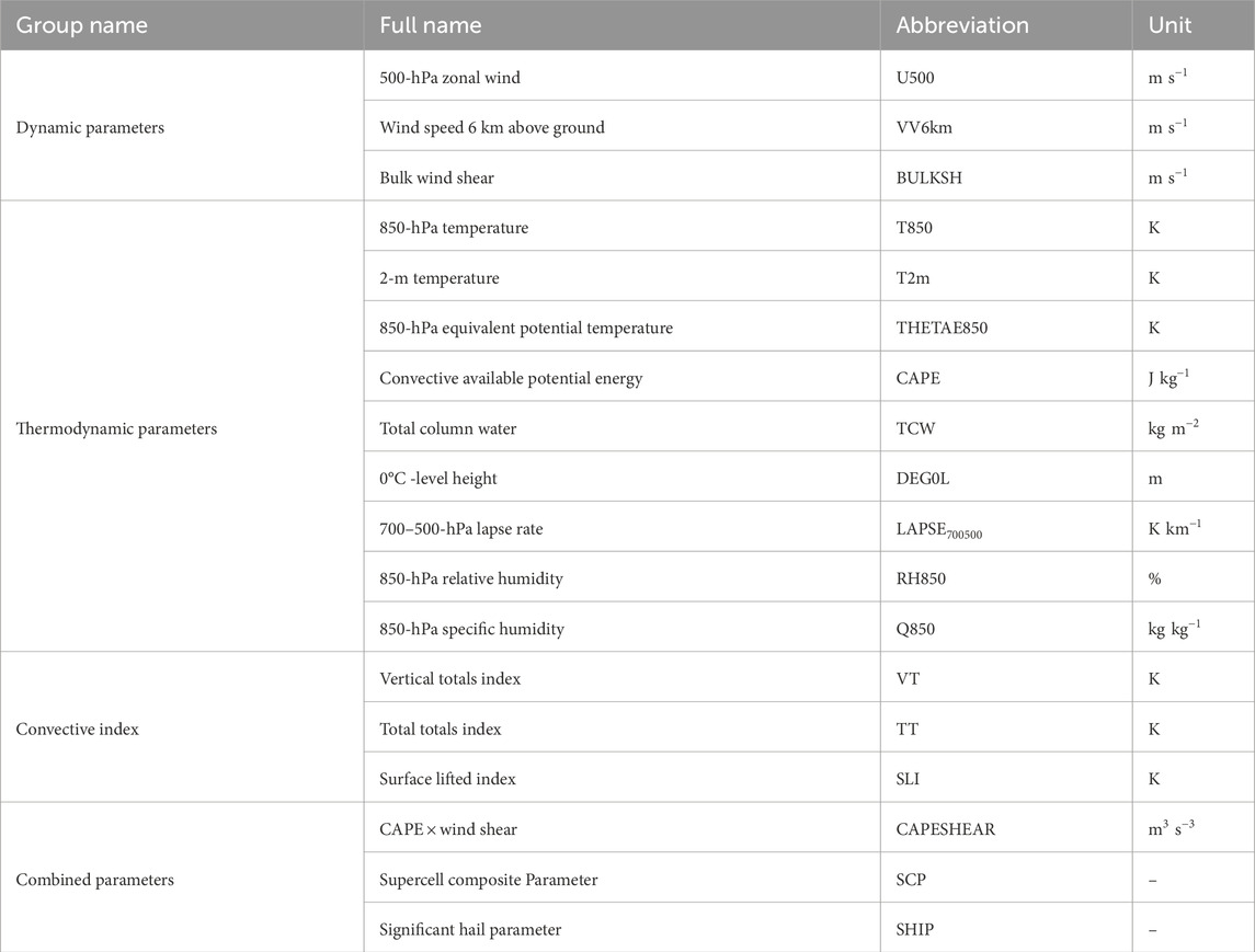
Table 1. List of parameters derived from ERA5 and their corresponding abbreviations.

To characterize the dynamic environment, we used the wind speed difference between 6 km and the surface (termed bulk wind shear, BULKSH), wind speed 6 km above ground (VV6km) and zonal wind at 500 hPa in our ML model. Wind speed and shear, such as BULKSH, are critical for the organization of convective systems in terms of single cells, multicells or supercells, the latter being capable of producing the largest hailstones (Markowski and Richardson, 2011). Results from Dennis and Kumjian (2017) and Kumjian et al. (2021) showed that increased shear produces increased hail mass due to three factors: (i) a larger updraft volume over which microphysically relevant hail processes can operate; (ii) increased hailstone residence times within the updraft; and (iii) a larger potential embryo source region. Thermodynamic parameters are highly relevant for the convective processes, the strength of the updraft related to thermal instability, and the life cycle of the cells (Markowski and Richardson, 2011; Wilhelm et al., 2023). Therefore, we considered nine different thermodynamic quantities: temperature and moisture at different vertical levels, total column water, lapse rate, and CAPE. Temperature and moisture content at different levels, and hence composite indices such as vertical totals (VT) or total totals (TT), determine thermal stability at mid-tropospheric levels. VT also describes conditional instability (Miller, 1975), often found in preconvective environments, and indicates the presence of CAPE. Total column water feedbacks on both updraft strength and supersaturated liquid water availability, both of which increase hail probability and hail size, but in a non-linear manner (Li et al., 2017). Lapse rate at mid-troposphere levels, e.g., between 700 and 500$\mathrm{h}\mathrm{P}\mathrm{a}$ (${\text{LAPSE}}_{700500}$), determines the stability of the lower troposphere (Kunz et al., 2020). The water droplets are taken through the lift of strong updraft to higher altitudes where temperatures are below freezing, freeze and accumulate layers of ice, eventually forming hailstones. CAPE largely controls the strength of the updraft, with greater CAPE favouring storms that produce larger hail. However, larger CAPE does not equate to larger hail and the nuances of storm structure must be examined (Lin and Kumjian, 2022). Composite parameters, such as CAPESHEAR, the supercell composite parameter SCP (Thompson et al., 2003), or the significant hail parameter SHIP (Allen et al., 2015), combine convective parameters known to be conducive to SCS/hail and are designed to capture severe hail environments.

According to several studies, both convective indices and combined convective parameters are well suited for ingredient-based predictions of SCSs (e.g., Haklander and Van Delden, 2003; Kunz, 2007; Taszarek et al., 2020; Kunz et al., 2020). Kunz (2007), for example, showed that the Surface Lifted Index (SLI) exhibits a high prediction skill for damaging hailstorms in southwestern Germany. Westermayer et al. (2017) found that SLI is related to the frequency of lightning within convective storms. Because it was shown in several studies (e.g., Brooks et al., 2003; Púčik et al., 2015) that large hail is most likely for the combination of high CAPE and high DLS, we use the product of the square root of CAPE $\times$ BULKSH (CAPESHEAR). The supercell composite parameter (SCP) highlights the co-existence of ingredients favoring SCSs on the basis of CAPE, storm relative helicity and bulk wind difference over the lower half of the storm depth. The significant hail parameter (SHIP), which is the product of CAPE, humidity, instability, temperature and wind shear, was often used to assess the likelihood and severity of hailstorms (Allen et al., 2015; Prein and Holland, 2018). In the research of Czernecki et al. (2019), this parameter improved the performance of ML models trained to predict large hail events. Overall, our selected 18 parameters show a large overlap to those selected in their study.

3.2 ML model

Combining reanalysis data with radar-based remote sensing and applying ML, particularly a CNN (Czernecki et al., 2019; Gagne et al., 2019), shows a high potential for improving the prediction of hailstorms, possibly outperforming conventional statistical prediction methods. The CNN in this study consists of a sequence of layers (Figure 2): a convolutional layer (Conv2D) followed by max-pooling and then a dropout layer. Max-pooling (MaxPool) is used to reduce the spatial dimensions of feature maps by selecting the maximum value within a defined window. Adding the dropout layer serves to reduce the risk of overfitting. This sequence is repeated once, and a final convolutional layer is added afterwards. All convolutional layers in this neural network have a kernel size of $3\times 3$ and use the Rectified Linear Unit (ReLU) activation function (Glorot et al., 2011). The ReLU function interprets only the non-negative part of its argument, aligning with the positive nature of hail-affected areas. The first and last two convolutional layers have 32 and 64 filters, respectively. The input data are both standardized using the Z-score normalization, such that it has a mean of 0 and a standard deviation of 1.

Figure 2

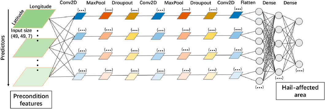
Figure 2. Schematic structure of the convolutional neural network with different layers used in this study and the number of nodes in this ML model is omitted (Ellipses).

The network incorporates two max-pooling layers to downsample feature maps (atmospheric fields here), with a $2\times 2$ pooling size and a stride of 2, i.e., the filters are moved by two grid points at each convolutional step. Two dropout layers with a dropout rate of 0.2 are utilized, where the dropout rate represents the fraction of features not being used. The first dense layer with ReLU activation and the second dense layer without an activation function have 64 and one nodes, respectively. Models are trained using ‘Adam’ optimization (Kingma and Ba, 2014). As a loss function and to estimate the best predictors, we use the lowest Mean Absolute Error (Willmott and Matsuura, 2005) of the hail-affected area.

The training and validation period includes all years from 2005 to 2017, whereas the testing period covers 2018–2019. The training of the CNN is done in a cross-validation setup with 30 training epochs. Cross-validation is performed iteratively: In a first loop, the CNN model is trained on the 11-year period 2007–2017, and the period 2005–2006 is taken for validation. The 2-year validation period changes to 2006–2007 in the second loop, and the training period of 11-year changes to 2008–2017 and 2005. The cross-validation includes 11 iterations until all possible evaluation periods are validated.

3.3 Verification measures

To evaluate the ML forecasts with respect to the hail-affected area in Germany, we use the MAE as the central verification metric. In addition, we decided to separately define individual large hail events exceeding a minimum hail-affected area yielding categorical forecasts for these events. In assessing non-probabilistic forecasts for discrete variables, a common approach is categorical verification (Murphy, 1996) based on contingency tables. The contingency table classifies elements $a-d$ based on whether an event was observed in the radar-derived tracks (Yes/No) and whether it was predicted by the ML model (Yes/No): $(a)$ number of correct hits, $(b)$ false alarms, $(c)$ misses/surprise events and $(d)$ correct non-events.

While several verification measures exist for evaluating binary events, there is no single perfect measure that captures all aspects of the model’s robustness without compromising others. Hence, seven verification measures and skill scores, derived from contingency tables, were computed to evaluate the model performance for the events (Table 2). The Critical Success Index (CSI) assesses the count of accurate hits compared to all events taken from the forecast or observations, i.e., leaving out many trivial correct non-events for something as rare as hail. As a result, the CSI provides a measure of the conditional probability of correct hits (Jolliffe and Stephenson, 2012; Czernecki et al., 2019). The Heidke Skill Score (HSS) shares similarities with the proportion correct (PC), but uses the forecast performance achieved by a random model as its baseline. The HSS is appropriate for the verification of rare events (Wilks, 2011). An HSS equal to 0 means that the skill of the model is as good as that of a random model. The Peirce Skill Score (PSS) is similar to HSS, while it is independent of the climatological event frequency. PSS is somewhat biased toward the Probability of detection (POD), making it more applicable for events that occur more frequently (Woodcock, 1976). With the highest value of HSS, PSS, POD, as well as the lowest False Alarm Ratio (FAR), the optimal threshold to distinguish small and large hail events can be determined comprehensively.

Table 2

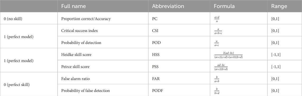
Table 2. Verification measures and skill scores used for this study including their abbreviations, formulas and ranges Wilks (2011). $n(=a+b+c+d)$ is the total number of samples.

4 Relation between hailstorms and ambient conditions

During the study period, a total of 911 hail days and 1,591 non-hail days (no track identified in the domain) are identified. Most of the potential hail tracks occur during daytime (12–18 UTC), which is in line with Kunz et al., 2009; Mohr and Kunz, 2013; Kunz et al., 2020). Therefore, we consider the environmental conditions from ERA5 at 12 UTC, but perform also comparisons for the 18 UTC fields.

In a first step, we analyse mean fields of environmental parameters over Germany during all days and on hail days only with the intention to identify spatial features favourable for hailstorms.

For the entire period 2005–2019 (Figure 3), hail hot-spots occur mainly over southern Germany: the federal State of Bavaria, Hessen, Baden-Württemberg and North Rhine-Westphalia. Many climatological mean fields of convective parameters are hardly geographically consistent with the climatology of hail hot-spots. However, on actual hail days (i.e., at least one identified potential hail track in the domain) some of these parameters are significantly different from the climatological mean state.

Figure 3

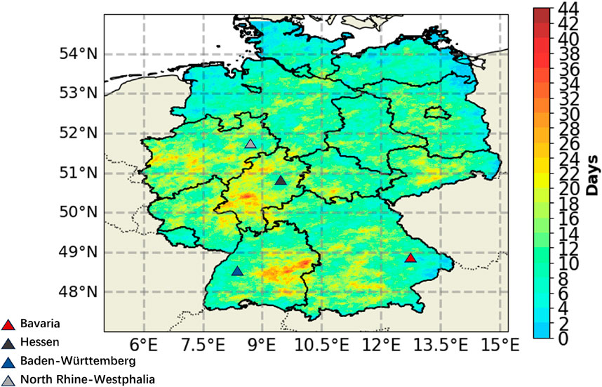
Figure 3. Accumulated hail-days derived from radar reflectivity of the DWD radar network over Germany from 2005 to 2019.

For example, Figure 4A illustrates the climatological mean field of CAPESHEAR at 12 UTC (all days from April to September 2005–2017), which will be identified later as the best single predictor (see Sect. 6). Relatively low values of CAPESHEAR are found in the northern part of Germany. The area with larger CAPESHEAR values is mostly located in southern Germany, especially in Baden-Württemberg and the southern part of Bavaria. Here, the climatological mean CAPESHEAR locally exceeds 1,500 ${\mathrm{m}}^{\mathrm{2}}{\mathrm{s}}^{-\mathrm{2}}$ which has been identified as a critical value for hail occurrence (Púčik et al., 2021). The reason for the large difference between northern and southern Germany is the climatologically lower temperature and lower moisture availability in northern Germany.

Figure 4

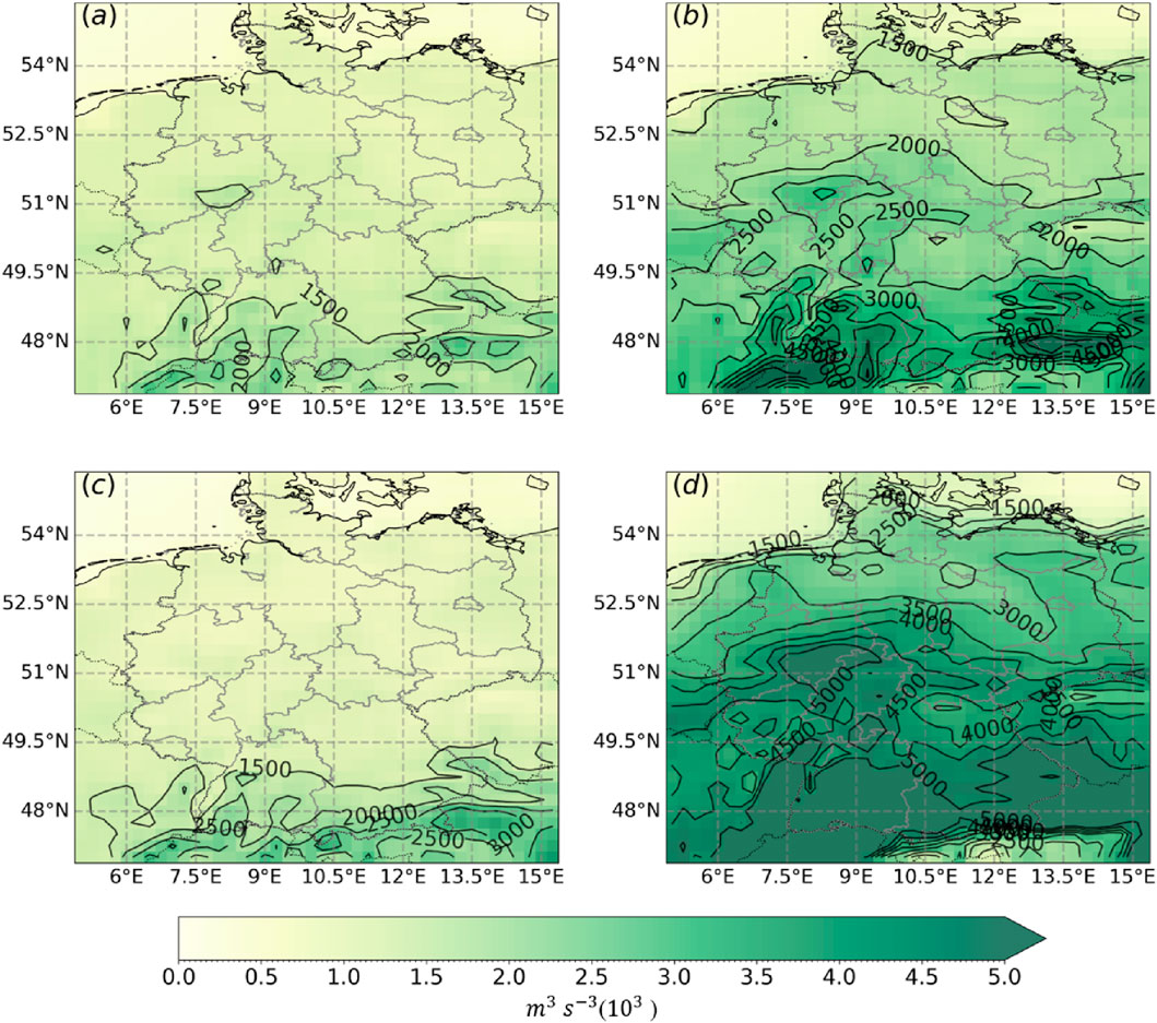
Figure 4. Mean fields of CAPESHEAR during the hail season April–September for the training period from 2005 to 2017. (a) Mean field for all days and (b) without non-hail days. (c) Mean for hail days below the lower tercile ranking of the daily affected area accumulation, and (d) for hail days above the upper tercile ranking. The contoured black lines highlight where values of CAPESHEAR larger than 1,500 ${\mathrm{m}}^{\mathrm{2}}{\mathrm{s}}^{-\mathrm{2}}$ indicate a tendency of very active convection (Púčik et al., 2021).

To focus on the convective conditions prior to hail occurrence, the mean field for hail days only is calculated (Figure 4B). Note, that the magnitude of CAPESHEAR is dominated by CAPE because of the much larger range of values compared to BULKSH. Higher CAPESHEAR values can be seen in northern, central, and southern Germany, but the spatial pattern with an increase from north to south remains similar, which is consistent with the statement that the hail frequency (Figure 3) in Germany generally increases from north to south (Punge and Kunz, 2016; Puskeiler et al., 2016). To further test our assumption that larger affected areas are associated with larger values of CAPESHEAR, the hail-only situation (Figure 4B) is subsampled and divided into three terciles (large, medium, small) based on the values of the daily hail-affected area. CAPESHEAR values over Germany (Figures 4C, D) with near climatological values during the lower tercile events and higher values during upper tercile events confirm this assumption. Highest CAPESHEAR values occur over the mountain ranges in Baden-Württemberg, Bavaria, and northern Hesse (Figures 3, 4D) which is consistent with an observed climatologically high hailstorm frequency at and downstream of these mountain ranges (Kunz and Puskeiler, 2010; Fluck et al., 2021).

The mean fields of other thermodynamic or combined parameters, such as CAPE, SHIP, or TT, show a distinct north-to-south gradient (not shown), similar to that for CAPESHEAR. In contrast, the variables that represent the general atmospheric background, such as U500, T850, do not show a pronounced north-to-south gradient for the mean field distributions (not shown).

The spatial distributions of the convection-related parameters primarily indicate that the general prerequisites for SCSs are given. However, they fall short in providing a robust relation to the hail-affected areas. To scrutinize the relation between potential hail tracks and convective ambient conditions, we correlate spatial fields of all 18 atmospheric parameters listed in Table 1 gridpoint-wise with the daily hail-affected area. Table 3 shows the mean Spearman’s rank correlation coefficients averaged over all gridpoints across Germany, which is not only helpful to identify the parameters that are most important for hailstorm prediction, but also gives some hints for the later selection of single convective parameters that are potentially most important for the ML model. Absolute correlation values are less than 0.5 for all selected parameters. This is mainly due to the fact that also non-hail days are included, which are more frequent and thus dominate the correlation. As the dynamic parameters U500 and BULKSH are relevant only on days with any kind of instability prevailing, their correlation coefficients are among the lowest of all parameters. Note that low correlation values do not necessarily imply that these parameters are unrelated to hailstorms on the local scale, since this analysis focuses on the spatial mean correlation between these parameters and the daily hail-affected areas, rather than pinpointing the exact locations of individual hailstorms.

Table 3

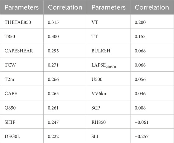
Table 3. Spatial mean Spearman’s rank correlation coefficients between daily hail-affected area and different convection-related parameters from ERA5 at 12 UTC in Germany for the period 2005–2017. The values of parameters are listed from positive to negative.

5 Model training and evaluation

To identify the best predictors for the CNN models out of all 18 predictor variables, we used a stepwise feature selection method. That is, we iteratively add predictors and always keep the predictors yielding the lowest MAE, and eventually end up with a combination of up to 7 parameters until the model prediction rarely gets much improvement (Mohr et al., 2015; McGovern et al., 2019; Quinting and Grams, 2021). The MAE decreases continuously by around 10% from using the single best predictor—CAPESHEAR—to the inclusion of 7 predictors (Figure 5). For the model, CAPESHEAR is the most important single predictor for the hail-affected area during test period (Figure 5), outperforming other convective parameters such as VT or TT. This is presumably due to its consideration of both thermodynamic and dynamic information of the environment. CAPESHEAR represents a combination of CAPE and BULKSH, both of which are critical factors in hail formation. CAPE quantifies the energy available for convection, which can lead to strong updrafts necessary for hailstone development (Battaglioli et al., 2023). Vertical wind shear, on the other hand, contributes to storm organization and longevity by separating updrafts and downdrafts, preventing storm weakening. Their combined role enhances the potential for robust and sustained convection, making it a significant predictor for hail occurrence in central Europe (Kunz et al., 2020). The combination with Q850, U500, BULKSH, and instability indices (VT, TT) yields the best model in terms of the MAE. The performance improves progressively with the number of predictors included, particularly after consideration of the second best predictor, Q850. The MAEs largely decrease once the second best predictor Q850 is selected, as it serves as a proxy for low-level moisture, a critical ingredient for storm initiation and intensification. This is also likely due to the fact that Q850 is not directly reflected by CAPESHEAR. Therefore, this addition yields a relative improvement of $6\%$ in model performance. VV6km reflects the strength of upward motion in the mid-troposphere, associated with the residence time of hailstones in the supercooled layers, influencing hail growth; while U500 normaly indicates mid-level flow patterns, which can influence storm propagation and organization. Including VV6km, U500, and BULKSH reduces the MAE only slightly, as they are highly correlated (Wilhelm et al., 2023).

Figure 5

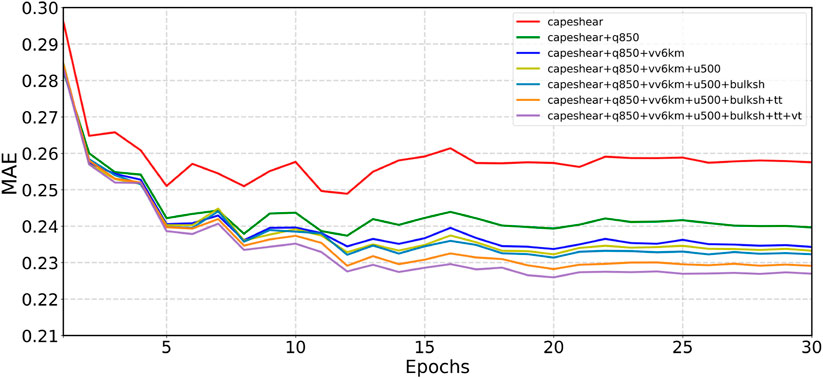
Figure 5. Model performance (measured in MAE) for different combinations of convective predictors (see legend) at $12\mathrm{U}\mathrm{T}\mathrm{C}$ using the method of the stepwise feature selection. Standardized MAEs are unitless.

Most of the important predictors describe the dynamical rather than the thermodynamical characteristics of the environment. This finding is in agreement with the studies of Westermayer et al. (2017)and Kunz et al. (2020), who showed that dynamical proxies are not only relevant for the prediction of hailstorms, but also decisive for their persistence or the length of the streaks, respectively. In addition, increased dynamical forcing is associated with either the presence of a synoptic cold front or a nearby jet stream, both leading to forced ascent of air masses. The study of Wilhelm et al. (2023) indicates the high correlation between BULKSH and U500, while BULKSH and U500 as single parameters have a very low prediction skill for the hail-affected area (see Sect. 4). Using ERA5 reanalysis at 18 UTC instead of 12 UTC, the seven best predictors yield MAEs comparable to those of the 12 UTC model (not shown). The 18 UTC ML model uses almost the same parameters, except for the replacement of Q850 with RH850.

During the model training, a major challenge in the ML-based prediction is the rare occurrence of hail events with a large effected area. However, these events may be most impactful in terms of the damage they might cause and thus reliable predictions are desirable. Accordingly, we use a density-based weighting for regression tasks introduced by Steininger et al. (2021). In brief, its main effect is to give rare data points more influence on the model training compared to common data points. The central parameter for the density-based weighting is $\alpha$, with $\alpha =0$ meaning that all data points receive the same weight and $\alpha \ge 1$ meaning that the most uncommon values receive much more weights than common values. For a detailed description, the interested reader is referred to the original publication by Steininger et al. (2021).

According to Figure 6A, which shows the daily hail affected area predicted by the CNN models and the observational data during the test period, non-hail days are most frequent. The figure also clearly reveals that on individual days the affected area may reach values up to 55,000 ${\text{km}}^2$. In terms of MAE, $\alpha =0.5$ yields a good compromise while marginally improving the ability of the ML model to capture the observed most extreme events. The very severe hail days in terms of large affected areas greater than $\mathrm{20,000}{\mathrm{k}\mathrm{m}}^2$ are still not captured adequately by the ML model, indicating a noteworthy limitation. Nevertheless, predictions for spatial extents of $\le \mathrm{20,000}{\mathrm{k}\mathrm{m}}^2$ using $\alpha =0.5$ show a moderate level of improvement in terms of successful prediction on daily hail-affected area with an overall better agreement with the observations. By gradually increasing the $\alpha$ values from 0 to 1.5, the ML model better detects extreme events on specific days (not shown), but at the cost of significantly overestimating the prediction of non-hail days. Overall, increasing $\alpha$ values results in higher MAE (Figure 6B). Thus, one can see that the overprediction of non-hail events has a largely negative impact on the overall MAE of the prediction. For the remainder of this study, all results are shown for $\alpha =0.5$, for which validation MAE is quasi the same as without weighting during the model training.

Figure 6

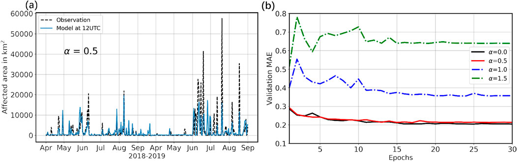
Figure 6. (a) Hail-affected area predicted from ambient conditions at $12\mathrm{U}\mathrm{T}\mathrm{C}$ in the test period (2018–2019) during the hail season with $\alpha =0.5$; the blue solid line is the ML prediction and the black dashed line is the observation for comparison. (b) Model performance in terms of MAE as a function of training iterations (epochs) during the validation period with different values of $\alpha$. MAEs are given for Z-normalized data and thus unitless.

It is noteworthy that the ML model using the ERA5 parameters at $12\mathrm{U}\mathrm{T}\mathrm{C}$ exhibits a marginally higher performance for the prediction of extreme events (larger hail affected area) compared to the $18\mathrm{U}\mathrm{T}\mathrm{C}$ counterpart (see Supplementary Figure S1 in the Appendix). However, the difference with respect to MAE between these two CNN models is marginal (see Supplementary Figure S2).

To estimate the performance of the ML model, it is compared with two simple non-ML reference models: Climatology-based forecast and short-term persistence forecast (Murphy, 1992; McGovern et al., 2023). The climatological forecast is taken here as the 30-day running mean hail-affected area for the period 2005–2019. The persistence forecast takes the hail-affected area from the previous day to predict the affected area for the current day, a benchmark for measuring the skill of forecasts produced by other methods, especially for very short-term forecasts. The skills of the models are compared to the ML model forecast by calculating the MAE between forecast and observations. Table 4 provides evidence that the predictive ability of the ML model is clearly superior to that of the two trivial reference models. The average MAE of 0.22 is an improvement of 54% over the persistence model forecast and 65% over the climatological model. The poor performance of the climatology-based model can be attributed to the fact that it predicts a small hail-affected area on each day, while strongly underestimating the affected area during severe events. Since climatology-based model will have almost continuous low values that verify with many zeros and then with larger areas, leading to a larger range of MAEs. Persistence-based model essentially has many zero forecasts and then short blocks of larger hail-affected areas. So at the beginning of occurrence of a hailstorm, the model will forecast a zero, at the end, a considerable area and verifies with a zero. The persistence model incorporates sequences of no hail days with no significantly large contribution to MAE, giving an overall better score.

Table 4

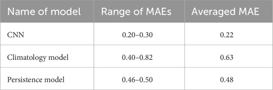
Table 4. Summary of the performance measures for CNN, climatology and persistence models. The MAEs are normalized (Z-normalization) and thus unitless.

Finally, categorical verification is applied to evaluate the performance of the CNN model for small and large hail events. Prior to identifying appropriate thresholds to distinguish between small and large hail events on the basis of observational data, the predictions of the CNN model are bias corrected by subtracting the averaged difference between model prediction and observation in the test period. After eliminating inherent biases (The averaged difference of daily hail-affected area of −298${\mathrm{k}\mathrm{m}}^2$) in the model, the resulting thresholds more likely align with the observed value of the hail-affected area. Figure 7A shows the different categorical skill scores for the CNN model as a function of hail-affected areas after the bias correction. For a threshold of 2,000${\mathrm{k}\mathrm{m}}^2$ the model exhibits high POD, high HSS, and high PSS while at the same time keeping the FAR below 0.4. The optimal threshold to separate between small and large events was found for a hail-affected area of 1,740${\mathrm{k}\mathrm{m}}^2$ (dark-red vertical line in Figure 7A). At this threshold HSS and PSS are maximized, while at the same time minimizing the FAR. For the above stated threshold, HSS is 0.66, PSS is 0.69 and FAR is only 0.3. For the same threshold of the hail-affected area, the HSSs of the forecast climatology and the persistence forecast are 0.51 and 0.36, respectively. The accuracy of the ML model was even found to be $88\%$ with POD = 0.78 and CSI = 0.58. Those skill scores are calculated from the actual contingency table (Figure 7B) based on the number of hail events. The ML model successfully identifies 56 hit cases (large hail-affected area) and correctly recognizes 241 non-events (small hail-affected area). However, it misses 16 large events and incorrectly classified 24 non-events. The slightly better model performance taking ambient conditions at $18\mathrm{U}\mathrm{T}\mathrm{C}$ is listed in the supplementary data for comparison purposes (Supplementary Figure S3).

Figure 7

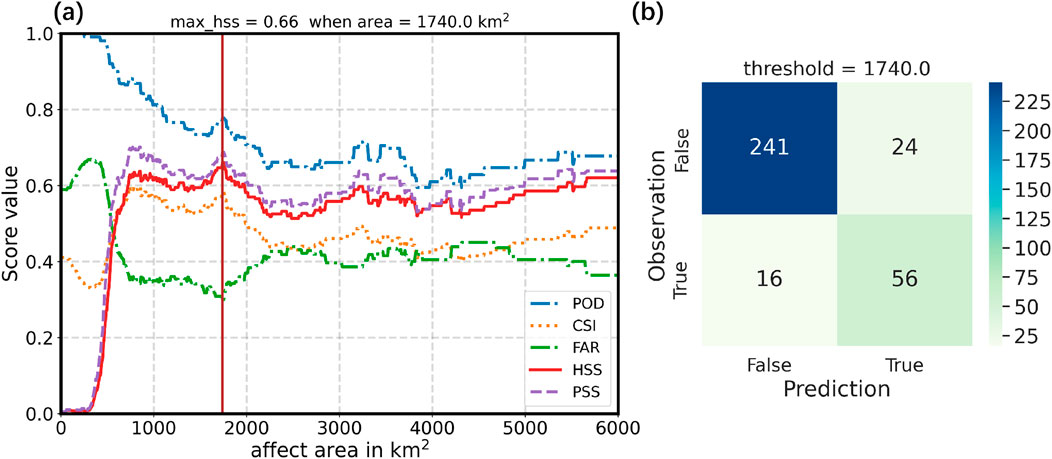
Figure 7. Categorical verification measures for large hail events during the test period (2018–2019). (a) Different skill scores (see legend and description in Section 3.3) as a function of the threshold used to distinguish between small and large hail events. (b) Contingency table for the optimal threshold of 1740 $\mathrm{k}{\mathrm{m}}^{\mathrm{2}}$ (marked in panel (A) with a red vertical line). True: high affected-area day >1740 $\mathrm{k}{\mathrm{m}}^{\mathrm{2}}$; False: little affected-area day <1740 $\mathrm{k}{\mathrm{m}}^{\mathrm{2}}$.

6 Interpretation of ML model

In this section, we compare situations during which the ML model succeeds and fails in predicting large hail events in order to better physically understand the different contributions of hail predictors in terms of ML prediction.

6.1 Class activation mapping: A case study

Even if the ML model with seven parameters from ERA5 reanalyses has a high prediction skill overall, the question remains during which ambient conditions CNN models can correctly predict large hail-affected areas. A widely-used diagnostic to unveil the relation of predictors and predictions is the gradient-weighted class activation mapping (Chollet, 2021). This method is useful to understand the causes leading to successful/failed predictions of the accumulated hail-affected area. The Grad-CAM utilizes gradient information from the last convolutional layer to generate a coarse localisation map, which highlights important regions in the input data for predicting how large the hail-affected area will be on a certain day. By overlaying the coarse localisation map with the features (Selvaraju et al., 2017), areas of particular importance can be visually identified. The corresponding heatmaps show where and which predictors have more significant weighting in the combination of the predictors.

Two case studies for an incorrect and a correct prediction were selected to better illustrate the problem at hand: 13 and 15 May 2018 (see Figure 8). During this period, a weak easterly flow on the south-eastern flank of a blocking anticyclone prevailed over Germany, in which an unstable air mass was encapsulated. The combination of strong vertical wind shear and the advection of filaments of potential vorticity associated with vertical lifting resulted in serial clustering of several SCS including hailstorms (Mohr et al., 2020). On 13 May (Panel a–h in Figure 8), CAPESHEAR (Figure 8G) spatially matches the maximum value of the corresponding activation heatmap (Figure 8H). This qualitatively good match was found for other successfully-predicted hail-days in the test period (not shown) and confirms CAPESHEAR being a good predictor for the CNN models. Convective predictors like VT (Figure 8E), TT (Figure 8F), or other environmental fields exhibit varied contributions to the hail activation heatmaps. Most of the time, regions with higher predictor values consistently align with higher activation values. Note that the ML model predicts daily hail-affected area totals without the specific hailstorm location information. Still the activation heatmaps often exhibit maximum values in regions where the actual hailstorms occurred indicating that they could be used to predict the location of hailstorms. Such an analysis, however, goes beyond the scope of this study.

Figure 8

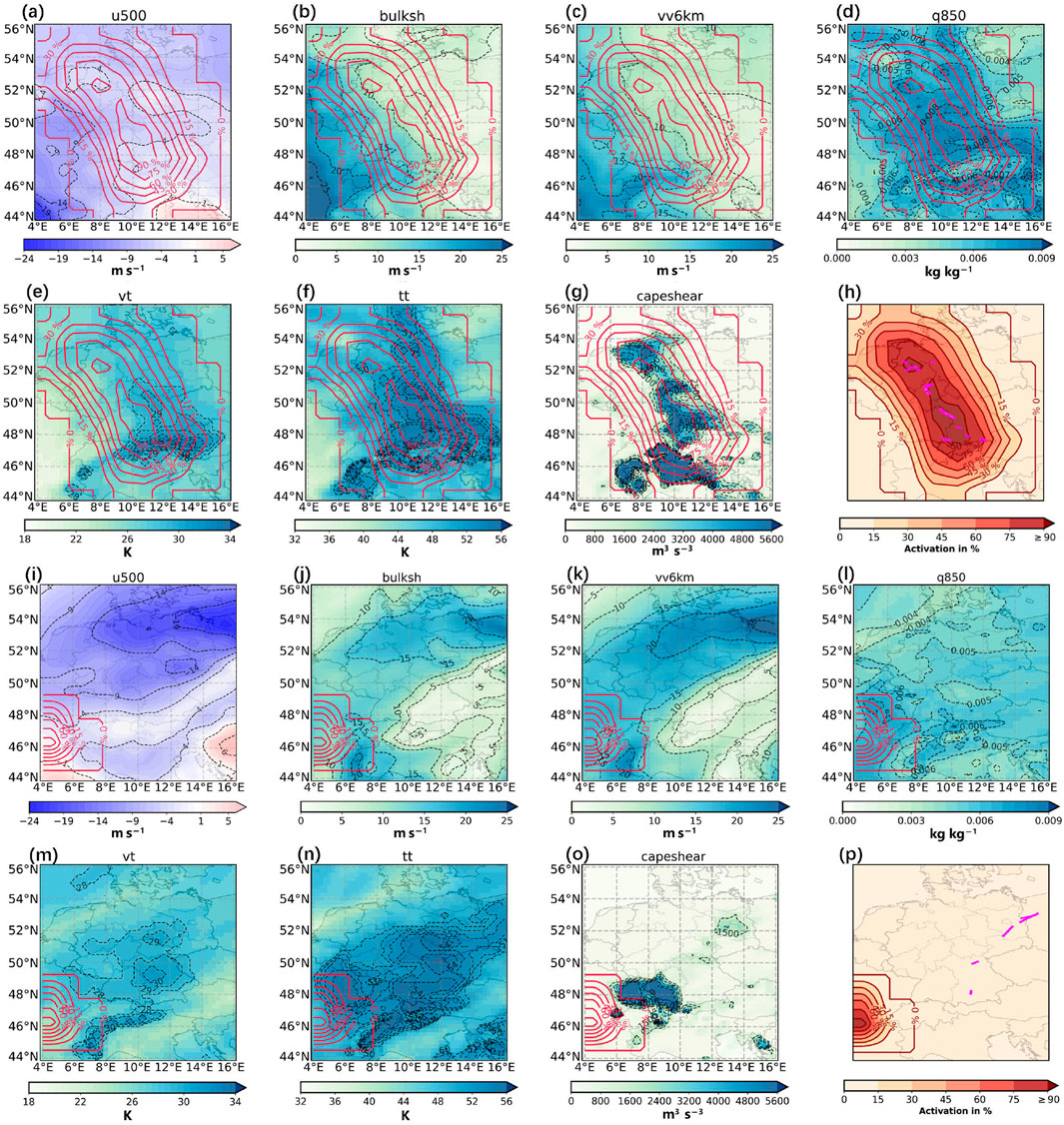
Figure 8. Different ambient conditions (blue shading) at $12\mathrm{U}\mathrm{T}\mathrm{C}$ for two case studies of a good forecast [13 May 2018; (a–h)] and a false alarm [15 May 2018; (i–p)]. The 7 predictors (a–g; i–o) are indicated in the title of each subplot overlapped with shaded heatmaps of class activation (h, p). Pink polygons in (h, p) represent the hail-affected area by every single hail track on that day. For VT, TT and CAPESHEAR only, the contoured areas are only favorable for the active convective and the development of thunderstorms. The activation (in %) of the CNN (red shading and solid contours every 15%) demarcates regions that hold significant relevance for the CNN decision-making.

For 15 May 2018, the ML model encountered difficulties in predicting hail events (Panel i–p in Figure 8), despite the presence of large-scale atmospheric conditions similar to that on 13 May (Mohr et al., 2020). SCS/hailstorms predominantly impacted the northeastern region of Germany. Despite enhanced BULKSH (Figure 8J) and VV6km (Figure 8K) near the hailstorms environmental conditions where characterized by low CAPESHEAR (Figure 8O) in the area of the events. The ML model’s prediction accuracy was comparably low in this case, as its prediction was dominated by the low CAPESHEAR values. The model’s highest activation (Figure 8P) was observed in the southwestern corner, where CAPESHEAR was relatively high, leading to an inaccurate prediction. This occurred despite favorable moisture conditions (Q850, Figure 8L) and atmospheric instability (VT, Figure 8M; TT; Figure 8N) being concentrated in central Germany indicating a too strong reliance of the model on CAPESHEAR.

Comparing the two case studies discussed, it is apparent that on 13 May hailstorm events were largely confined to specific geographical zones, primarily occurring between 12 and 16 UTC. In contrast, on 15 May, characterized by an inaccurate ML model prediction, hailstorms, while also concentrated between 12 and 15 UTC, exhibited a wider geographical distribution and had shorter duration. The negative values in U500 near the observed hailstorms are associated with the blocking in the middle troposphere, leading to fewer severe organized convective systems (Mohr et al., 2020). This highlights one synoptic pattern during which the ML model has difficulties in predicting the hail affected area on a specific day.

6.2 Class activation mapping: Systematic analysis

As mentioned previously, most successful predictions of the hail-affected area are obtained when hailstorms occur in form of spatial-temporal clusters. A statistical approach to identify prevalent convective patterns for hailstorms (Kunz et al., 2020) can improve our understanding of the interplay between prevailing conditions and predictions of the hail-affected area. In total, 56 accurately predicted hailstorm cases and 16 false alarm cases, along with their corresponding activation heatmaps, are analysed in the following (Supplementary Figure S4). The results reveal no obvious differences in terms of mid-level wind, wind shear (BULKSH, VV6km), and convective indices (VT, TT) between the two categories. However, cases with correct predictions exhibit notably higher CAPESHEAR, coupled with a large-scale westerly zonal wind at 500 hPa over Germany. False alarm cases lack these distinct features and show lower values of Q850, indicating less humid atmospheric conditions. One explanation might be that during hit cases, strong southerly winds, frequently associated with the Western side of blocking systems or ridges, tend to be stronger. In contrast, false alarms are often associated with the transition from weak westerly to weak easterly winds, which may be related to the weaker blocking systems. To conclude, if storms are sparse and occur in the distant regions far away from the strong convective activity, the CNNs struggle to correctly predict the affected area. Composite maps during hit cases show strong southwesterly winds on the Western side of upper-tropospheric ridges (not shown). Also it is noteworthy that the gradients in the false alarm are much weaker. So overall this indicates considerably weaker shear.

To quantify the significance of the seven predictors included in the ML prediction model, spatial correlations were computed between daily activation heatmaps and the corresponding environment fields of the predictors (Figure 9). The objective is to compare the contributions of individual predictors to the CNN models’ prediction in both correct forecasts and false alarms. For example, in the two case studies, the correlation matrix between the activation heatmap and the predictors U500, Q850, VT, TT, and CAPESHEAR shows relatively high correlation coefficients of 0.33, 0.57, 0.43, 0.61, and 0.46, respectively, on 13 May 2018 (Marked in Figure 9). Conversely, on 15 May 2018, the corresponding correlation coefficients are relatively low, measuring only 0.3, 0.39, −0.11, 0.12, and 0.14. Upon examining hail events categorized as correct or incorrect cases, it becomes clear that there is large variability in the correlation coefficients between different predictor fields and heatmaps.

Figure 9

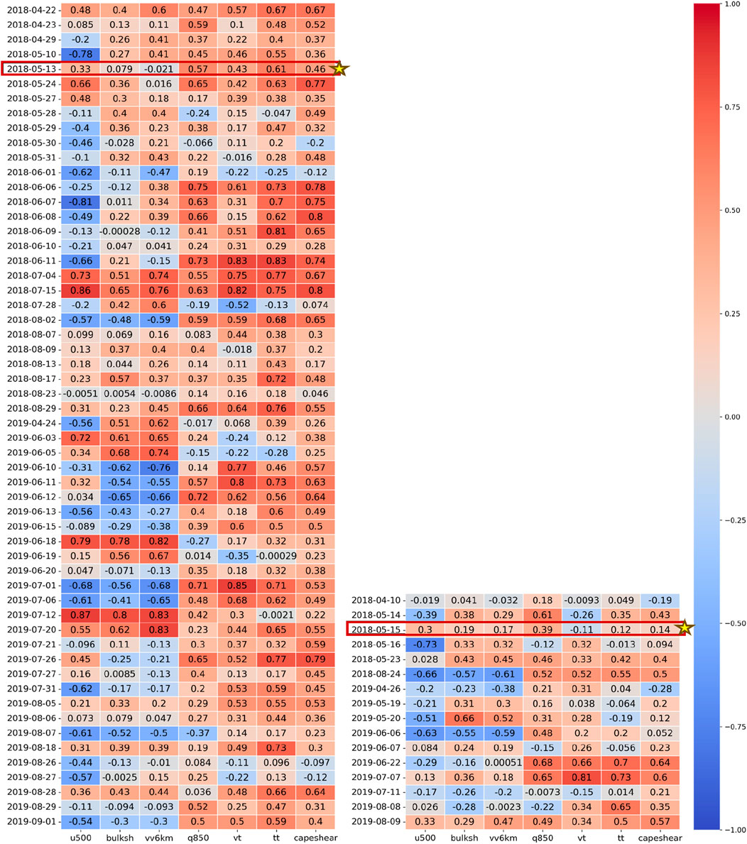
Figure 9. Correlation matrix between ambient predictors (Table 1) at 12 UTC and the activation heatmaps of 72 observed hail events. The left (right) is for 56 correct forecast events (16 false alarm events) in Figure 7B.

The boxplots (Figure 10) illustrate the distribution of the correlation coefficients between the activation heatmap and the different non-normalized convection-related parameters on a daily basis. It highlights a large variability of the correlation coefficients in the range between around −0.75 and +0.75, which complicate the prediction of the hail-affected area for individual events. CAPESHEAR in Figure 10A shows on average a high correlation with the activation heatmaps and a narrower distribution, which reaffirms its potential as a reliable predictor in ML applications for environmental conditions leading to hail. Conversely, the correlation coefficients for U500 exhibit a broader range and on average negative values. This indicates that CNN models can hardly gain predictive information from upper-level atmospheric flow solely, such as blocking, which indirectly affects the convective predisposition by influencing atmospheric instability (Mohr et al., 2019; Mohr et al., 2020). Hit cases (Figure 10A) experience stronger westerly winds associated with the northern side of blocking systems or ridges, while false alarm cases (Figure 10B) often show weak easterly winds, potentially linked to the northern edge of low-pressure systems.

Figure 10

Figure 10. Boxplots of the correlation matrix (Figure 9) between ambient predictors at 12 UTC and the activation heatmap of observed hail events for (a) correct forecasts and (b) false alarm events.

Furthermore, the consistently higher correlation coefficients for VT, TT, and CAPESHEAR for correct forecast events compared to false alarm events intuitively confirm the role and importance of these three parameters for the ML model’s predictive decisions. Further improvements might be possible by splitting the domain in multiple patches, for which different models have to be trained. Separate models for smaller patches could potentially account for the spatial variability of the hailstorms.

7 Conclusions and discussion

Adequate predictions of when, where, and how severe hailstorms will occur still pose a major challenge. In current operational NWP models hail is often not a default forecast parameter because it requires complex 2- or 3-moment microphysics schemes that are computationally very expensive. In addition, the transient nature of hailstorms further hinders accurate prediction in current models, and forecast errors can grow quickly (Snook et al., 2016). The primary objective of this study is hence to identify the most suitable predictors among a large set of convection-related variables for building an ML model capable of predicting the daily hail-affected area in Germany. The reference data are radar-derived hailstorm estimates for the period from 2005 to 2019 during the summer half-year from April to September. We divide the entire 15 years of ERA5 reanalysis and radar-identified potential hailstorm data into 13 years for training and validation (2005–2017) and 2 years for testing (2018–2019). Sensitivity experiments are carried out considering different times of day and 18 different convective parameters as potential predictors. These experiments lead to the identification of a set of seven predictors at 12 UTC (and 18 UTC). In the following, we provide answers to the questions raised in the Introduction:

1. The CNN model developed in this study offers potential to provide forecasts of the hail-affected area in Germany. In comparison to simple reference forecasts based on climatology and persistence, the CNN model exhibits a significantly higher skill measured here in terms of MAE of the hail-affected area. For events with large affected areas of at least 1,740 $\mathrm{k}{\mathrm{m}}^{\mathrm{2}}$, the CNN model exhibits a HSS of 0.66, along with a reasonable accuracy rate of 88% compared to the climatology-based (0.51 HSS) and persistence-based forecast (0.36 HSS), positioning it as a valuable tool for hail prediction. We assume that the prediction skill may even further increase after fine-tuning in future work.

2. From the 18 pre-selected convective parameter candidates, U500, BULKSH, VV6km, Q850, VT, TT, and CAPESHEAR are identified as the seven best predictors. Notably, CAPESHEAR not only shows a high correlation with the hail affected area, but also emerges as the best single predictor in the ML model. Among the parameters representing atmospheric dynamics, vertical wind shear plays an important role in the accuracy of the model predictions. Higher values of VT and TT also improve the ML model’s ability to successfully predict hail events, most likely because these parameters account for the atmospheric vertical instability during hail days. The inclusion of humidity parameters further improve the ML performance. Dynamical parameters, such as BULKSH and VV6km, are also of importance in the predictor selection. Despite being highly correlated with each other, the inclusion of both still slightly improve model performance. On the other hand, U500 alone, representing the large-scale atmospheric circulation at mid-troposphere levels, does not provide valuable predictive information for the ML model. Although different layers of wind-related parameters can benefit reflecting convective environments, additional but highly correlated layers of wind have been filtered out by using the stepwise feature selection method.

3. For isolated hailstorms or a small number of storms on a day in a weakly unstable environment, especially in regions with high CAPESHEAR values far from corresponding storm tracks, the ML model tends to produce inaccurate predictions. Looking at the synoptic conditions for the hit and false alarm cases, U500 shows noticeable differences between the two samples. The results indicate that during hit cases, westerly winds, frequently associated with the northern side of blocking systems or ridges, tend to be stronger. In contrast, false alarms are often associated with weak easterly winds, which may be related to the northern edge of low-pressure systems.

A major limitation of the chosen approach here is that the CNN model predictions only offer information on the integrated hail-affected area but not on the localization of individual hailstorms. Future studies could aim to develop ML models for such predictions, for example, by training on individual patches distributed across Germany. This would increase the model’s potential to be used for operational forecasting and warnings. Also, developing distinct ML models for different instability environments would be a potential avenue for future research. Environments with strong instability are typically dominated by well-defined convective processes, while weak instability environments may involve subtler dynamics, such as elevated convection or mesoscale lifting mechanisms. Tailored models could better capture the unique features of each regime, enhancing overall prediction accuracy. However, a limiting factor would be the reduction of the training and test data when splitting the events in different instability environments. Also, the classification into different instability environments would introduce strict thresholds which may degrade the models’ ability to generalize. An alternative approach would be the introduction of composite parameters specifically designed for weak instability environments. Different ML models for other optimization strategies could also be explored, for example, random forests, gradient boosting machines, or transformer-based architectures, might offer complementary advantages by taking into account temporal dependencies. Overall, the study shows promising results in the prediction skill of ML models for the daily hail-affected area. To our knowledge, no previous research has considered the spatial extent of hailstorms, which is—in combination with hail sizes—most relevant for the potential damage it may cause. Although the ML model can still be optimized, the feature selection of relevant parameters as well as the class activation mapping provide valuable insights for predictions of hailstorm occurrence and can give hints on the involved processes. Besides, it showcases how to combine CNNs with NWP models to improve hailstorm predictions and derive warnings in the future.

Data availability statement

The raw data supporting the conclusions of this article will be made available by the authors, without undue reservation.

Author contributions

SL: Methodology, Visualization, Writing–original draft, Writing–review and editing. PK: Supervision, Writing–review and editing. MK: Resources, Supervision, Writing–review and editing, Funding acquisition. JW: Supervision, Writing–review and editing. JQ: Funding acquisition, Supervision, Writing–review and editing.

Funding

The author(s) declare that financial support was received for the research, authorship, and/or publication of this article. The contribution of SL and JQ was partly funded by the European Union (ERC, ASPIRE, 101077260). MK is supported by the Helmholtz Association (Research Program “Changing Earth – Sustaining our Future”).

Acknowledgments

We thank Sebastian Lerch for the valuable suggestions on ML. We thank Fabian Mockert for assisting in setting up the class activation mapping. We thank ECMWF for providing ERA5 reanalysis data and Heinz Jürgen Punge for computing the convection-related parameters. DWD is acknowledged for radar data provision. We thank Manuel Schmidberger and Susanna Mohr for providing radar-based hail streak estimations. Finally, we are grateful for the helpful feedback of two reviewers.

Conflict of interest

The authors declare that the research was conducted in the absence of any commercial or financial relationships that could be construed as a potential conflict of interest.

The author(s) declared that they were an editorial board member of Frontiers, at the time of submission. This had no impact on the peer review process and the final decision.

Generative AI statement

The author(s) declare that no Generative AI was used in the creation of this manuscript.

Publisher’s note

All claims expressed in this article are solely those of the authors and do not necessarily represent those of their affiliated organizations, or those of the publisher, the editors and the reviewers. Any product that may be evaluated in this article, or claim that may be made by its manufacturer, is not guaranteed or endorsed by the publisher.

Supplementary material

The Supplementary Material for this article can be found online at: https://www.frontiersin.org/articles/10.3389/feart.2025.1527391/full#supplementary-material

References

Ackermann, L., Soderholm, J., Protat, A., Whitley, R., Ye, L., and Ridder, N. (2023). Radar and environment-based hail damage estimates using machine learning. Atmos. Meas. Tech. Discuss. 2023, 1–24. Available at: https://amt.copernicus.org/articles/17/407/2024/

Google Scholar

Allen, J. T., Tippett, M. K., and Sobel, A. H. (2015). An empirical model relating US monthly hail occurrence to large-scale meteorological environment. J. Adv. Model. Earth Syst. 7, 226–243. doi:10.1002/2014MS000397

CrossRef Full Text | Google Scholar

Aran, M., Pena, J., and Torà, M. (2011). Atmospheric circulation patterns associated with hail events in lleida (catalonia). Atmos. Res. 100, 428–438. doi:10.1016/j.atmosres.2010.10.029

CrossRef Full Text | Google Scholar

Auliya, M. N., Saputra, A. H., Kristianto, A., and Qomariyatuzzamzami, L. N. (2023). “Predicting hailstorms through machine learning approach using multiple source data analysis,” in International conference on radioscience, equatorial atmospheric science and environment (Springer), 225–236.

Google Scholar

Battaglioli, F., Groenemeijer, P., Tsonevsky, I., and Púčik, T.(2023). Forecasting large hail and lightning using additive logistic regression models and the ecmwf reforecasts. Nat. Hazards Earth Syst. Sci. Discuss. 2023, 3651–3669. doi:10.5194/nhess-23-3651-2023

CrossRef Full Text | Google Scholar

Brooks, H. E., Lee, J. W., and Craven, J. P. (2003). The spatial distribution of severe thunderstorm and tornado environments from global reanalysis data. Atmos. Res. 67, 73–94. doi:10.1016/s0169-8095(03)00045-0

CrossRef Full Text | Google Scholar

Burke, A., Snook, N., Gagne II, D. J., McCorkle, S., and McGovern, A. (2020). Calibration of machine learning–based probabilistic hail predictions for operational forecasting. Weather Forecast. 35, 149–168. doi:10.1175/waf-d-19-0105.1

CrossRef Full Text | Google Scholar

Chollet, F. (2021). Deep learning with Python (Simon and schuster).

Google Scholar

Czernecki, B., Taszarek, M., Marosz, M., Półrolniczak, M., Kolendowicz, L., Wyszogrodzki, A., et al. (2019). Application of machine learning to large hail prediction-the importance of radar reflectivity, lightning occurrence and convective parameters derived from era5. Atmos. Res. 227, 249–262. doi:10.1016/j.atmosres.2019.05.010

CrossRef Full Text | Google Scholar

Dennis, E. J., and Kumjian, M. R. (2017). The impact of vertical wind shear on hail growth in simulated supercells. J. Atmos. Sci. 74, 641–663. doi:10.1175/JAS-D-16-0066.1

CrossRef Full Text | Google Scholar

Dessens, J., Berthet, C., and Sanchez, J. (2015). Change in hailstone size distributions with an increase in the melting level height. Atmos. Res. 158, 245–253. doi:10.1016/j.atmosres.2014.07.004

CrossRef Full Text | Google Scholar

ECMWF (2023). Era5 - data documentation.

Google Scholar

Fluck, E., Kunz, M., Geissbuehler, P., and Ritz, S. P. (2021). Radar-based assessment of hail frequency in europe. Nat. Hazards Earth Syst. Sci. 21, 683–701. doi:10.5194/nhess-21-683-2021

CrossRef Full Text | Google Scholar

Gagne, D., McGovern, A., Jerald, J., Coniglio, M., Correia, J., and Xue, M. (2015). Day-ahead hail prediction integrating machine learning with storm-scale numerical weather models. Proc. AAAI Conf. Artif. Intell. 29, 3954–3960. doi:10.1609/aaai.v29i2.19053

CrossRef Full Text | Google Scholar

Gagne, D. J., Haupt, S. E., Nychka, D. W., and Thompson, G. (2019). Interpretable deep learning for spatial analysis of severe hailstorms. Mon. Weather Rev. 147, 2827–2845. doi:10.1175/mwr-d-18-0316.1

CrossRef Full Text | Google Scholar

Gagne, D. J., McGovern, A., Haupt, S. E., Sobash, R. A., Williams, J. K., and Xue, M. (2017). Storm-based probabilistic hail forecasting with machine learning applied to convection-allowing ensembles. Weather Forecast. 32, 1819–1840. doi:10.1175/waf-d-17-0010.1

CrossRef Full Text | Google Scholar

Glorot, X., Bordes, A., and Bengio, Y. (2011). “Deep sparse rectifier neural networks,” in Proceedings of the fourteenth international conference on artificial intelligence and statistics (JMLR Workshop and Conference Proceedings), 315–323. Available at: https://proceedings.mlr.press/v15/glorot11a.html

Google Scholar

Haklander, A. J., and Van Delden, A. (2003). Thunderstorm predictors and their forecast skill for The Netherlands. Atmos. Res. 67, 273–299. doi:10.1016/s0169-8095(03)00056-5

CrossRef Full Text | Google Scholar

Han, L., Liang, H., Chen, H., Zhang, W., and Ge, Y. (2021). Convective precipitation nowcasting using u-net model. IEEE Trans. Geoscience Remote Sens. 60, 1–8. doi:10.1109/tgrs.2021.3100847

CrossRef Full Text | Google Scholar

Handwerker, J. (2002). Cell tracking with trace3d—a new algorithm. Atmos. Res. 61, 15–34. doi:10.1016/s0169-8095(01)00100-4

CrossRef Full Text | Google Scholar

Hersbach, H., Bell, B., Berrisford, P., Hirahara, S., Horányi, A., Muñoz-Sabater, J., et al. (2020). The era5 global reanalysis. Q. J. R. Meteorological Soc. 146, 1999–2049. doi:10.1002/qj.3803

CrossRef Full Text | Google Scholar

Jolliffe, I. T., and Stephenson, D. B. (2012). Forecast verification: a practitioner’s guide in atmospheric science. John Wiley and Sons.

Google Scholar

Khain, A., Beheng, K., Heymsfield, A., Korolev, A., Krichak, S., Levin, Z., et al. (2015). Representation of microphysical processes in cloud-resolving models: spectral (bin) microphysics versus bulk parameterization. Rev. Geophys. 53, 247–322. doi:10.1002/2014rg000468

CrossRef Full Text | Google Scholar

Kingma, D. P., and Ba, J. (2014). Adam: a method for stochastic optimization. arXiv preprint arXiv:1412.6980.

Google Scholar

Kumjian, M. R., and Lombardo, K. (2020). A hail growth trajectory model for exploring the environmental controls on hail size: model physics and idealized tests. J. Atmos. Sci. 77, 2765–2791. doi:10.1175/JAS-D-20-0016.1

CrossRef Full Text | Google Scholar

Kumjian, M. R., Lombardo, K., and Loeffler, S. (2021). The evolution of hail production in simulated supercell storms. J. Atmos. Sci. 78, 3417–3440. doi:10.1175/JAS-D-21-0034.1

CrossRef Full Text | Google Scholar

Kunz, M. (2007). The skill of convective parameters and indices to predict isolated and severe thunderstorms. Nat. Hazards Earth Syst. Sci. 7, 327–342. doi:10.5194/nhess-7-327-2007

CrossRef Full Text | Google Scholar

Kunz, M., Blahak, U., Handwerker, J., Schmidberger, M., Punge, H. J., Mohr, S., et al. (2018). The severe hailstorm in southwest Germany on 28 july 2013: characteristics, impacts and meteorological conditions. Q. J. R. Meteorological Soc. 144, 231–250. doi:10.1002/qj.3197

CrossRef Full Text | Google Scholar

Kunz, M., and Puskeiler, M. (2010). High-resolution assessment of the hail hazard over complex terrain from radar and insurance data. Meteorol. Z. 19, 427–439. doi:10.1127/0941-2948/2010/0452

CrossRef Full Text | Google Scholar

Kunz, M., Sander, J., and Kottmeier, C. (2009). Recent trends of thunderstorm and hailstorm frequency and their relation to atmospheric characteristics in southwest Germany. Int. J. Climatol. A J. R. Meteorological Soc. 29, 2283–2297. doi:10.1002/joc.1865

CrossRef Full Text | Google Scholar

Kunz, M., Wandel, J., Fluck, E., Baumstark, S., Mohr, S., and Schemm, S. (2020). Ambient conditions prevailing during hail events in central europe. Nat. Hazards Earth Syst. Sci. 20, 1867–1887. doi:10.5194/nhess-20-1867-2020

CrossRef Full Text | Google Scholar

Leinonen, J., Hamann, U., Germann, U., and Mecikalski, J. R. (2022). Nowcasting thunderstorm hazards using machine learning: the impact of data sources on performance. Nat. Hazards Earth Syst. Sci. 22, 577–597. doi:10.5194/nhess-22-577-2022

CrossRef Full Text | Google Scholar

Li, M., Zhang, F., Zhang, Q., Harrington, J. Y., and Kumjian, M. R. (2017). Nonlinear response of hail precipitation rate to environmental moisture content: a real case modeling study of an episodic midlatitude severe convective event. J. Geophys. Res. Atmos. 122, 6729–6747. doi:10.1002/2016JD026373

CrossRef Full Text | Google Scholar

Lin, Y., and Kumjian, M. R. (2022). Influences of cape on hail production in simulated supercell storms. J. Atmos. Sci. 79, 179–204. doi:10.1175/JAS-D-21-0054.1

CrossRef Full Text | Google Scholar

Malečić, B., Prtenjak, M. T., Horvath, K., Jelić, D., Jurković, P. M., Ćorko, K., et al. (2022). Performance of hailcast and the lightning potential index in simulating hailstorms in Croatia in a mesoscale model–sensitivity to the pbl and microphysics parameterization schemes. Atmos. Res. 272, 106143. doi:10.1016/j.atmosres.2022.106143

CrossRef Full Text | Google Scholar

Manzato, A., Cicogna, A., Centore, M., Battistutta, P., and Trevisan, M. (2022). Hailstone characteristics in northeast Italy from 29 years of hailpad data. J. Appl. Meteorology Climatol. 61, 1779–1795. doi:10.1175/jamc-d-21-0251.1

CrossRef Full Text | Google Scholar

Markowski, P., and Richardson, Y. (2011). Mesoscale meteorology in midlatitudes. John Wiley and Sons.

Google Scholar

McGovern, A., Chase, R. J., Flora, M., Gagne, D. J., Lagerquist, R., Potvin, C. K., et al. (2023). A review of machine learning for convective weather. Artif. Intell. Earth Syst. 2, 1–61. doi:10.1175/aies-d-22-0077.1

PubMed Abstract | CrossRef Full Text | Google Scholar

McGovern, A., Lagerquist, R., John Gagne, D., Jergensen, G. E., Elmore, K. L., Homeyer, C. R., et al. (2019). Making the black box more transparent: understanding the physical implications of machine learning. Bull. Am. Meteorological Soc. 100, 2175–2199. doi:10.1175/bams-d-18-0195.1

CrossRef Full Text | Google Scholar

Miller, R. C. (1975). Notes on analysis and severe-storm forecasting procedures of the air force global weather central.

Google Scholar

Mohr, S., and Kunz, M. (2013). Recent trends and variabilities of convective parameters relevant for hail events in Germany and europe. Atmos. Res. 123, 211–228. doi:10.1016/j.atmosres.2012.05.016

CrossRef Full Text | Google Scholar

Mohr, S., Kunz, M., and Keuler, K. (2015). Development and application of a logistic model to estimate the past and future hail potential in Germany. J. Geophys. Res. Atmos. 120, 3939–3956. doi:10.1002/2014jd022959

CrossRef Full Text | Google Scholar

Mohr, S., Wandel, J., Lenggenhager, S., and Martius, O. (2019). Relationship between atmospheric blocking and warm-season thunderstorms over western and central europe. Q. J. R. Meteorological Soc. 145, 3040–3056. doi:10.1002/qj.3603

CrossRef Full Text | Google Scholar

Mohr, S., Wilhelm, J., Wandel, J., Kunz, M., Portmann, R., Punge, H. J., et al. (2020). The role of large-scale dynamics in an exceptional sequence of severe thunderstorms in europe may–june 2018. Weather Clim. Dyn. 1, 325–348. doi:10.5194/wcd-1-325-2020

CrossRef Full Text | Google Scholar

MunichRE(2020). MunichRE.

Google Scholar

Murphy, A. H. (1992). Climatology, persistence, and their linear combination as standards of reference in skill scores. Weather Forecast. 7, 692–698. doi:10.1175/1520-0434(1992)007<0692:cpatlc>2.0.co;2

CrossRef Full Text | Google Scholar

Murphy, A. H. (1996). The finley affair: a signal event in the history of forecast verification. Weather Forecast. 11, 3–20. doi:10.1175/1520-0434(1996)011<0003:tfaase>2.0.co;2

CrossRef Full Text | Google Scholar

Piper, D., and Kunz, M. (2017). Spatiotemporal variability of lightning activity in europe and the relation to the north atlantic oscillation teleconnection pattern. Nat. Hazards Earth Syst. Sci. 17, 1319–1336. doi:10.5194/nhess-17-1319-2017

CrossRef Full Text | Google Scholar

Prein, A. F., and Holland, G. J. (2018). Global estimates of damaging hail hazard. Weather Clim. Extrem. 22, 10–23. doi:10.1016/j.wace.2018.10.004

CrossRef Full Text | Google Scholar

Púčik, T., Groenemeiger, P., and Tsonevsky, I. (2021). Vertical wind shear and convective storms. European Centre for Medium-Range Weather Forecasts. Available at: https://www.ecmwf.int/en/elibrary/81211-vertical-wind-shear-and-convective-storms

Google Scholar

Púčik, T., Groenemeijer, P., Rỳva, D., and Kolář, M. (2015). Proximity soundings of severe and non-severe thunderstorms in Central Europe. Mon. Weather Rev. 143, 4805–4821. doi:10.1175/mwr-d-15-0104.1

CrossRef Full Text | Google Scholar

Pulukool, F., Li, L., and Liu, C. (2020). Using deep learning and machine learning methods to diagnose hailstorms in large-scale thermodynamic environments. Sustainability 12, 10499. doi:10.3390/su122410499

CrossRef Full Text | Google Scholar

Punge, H. J., and Kunz, M. (2016). Hail observations and hailstorm characteristics in europe: a review. Atmos. Res. 176, 159–184. doi:10.1016/j.atmosres.2016.02.012

CrossRef Full Text | Google Scholar

Puskeiler, M., Kunz, M., and Schmidberger, M. (2016). Hail statistics for Germany derived from single-polarization radar data. Atmos. Res. 178, 459–470. doi:10.1016/j.atmosres.2016.04.014

CrossRef Full Text | Google Scholar

Quinting, J. F., and Grams, C. M. (2021). Toward a systematic evaluation of warm conveyor belts in numerical weather prediction and climate models. part i: predictor selection and logistic regression model. J. Atmos. Sci. 78, 1465–1485. doi:10.1175/jas-d-20-0139.1

CrossRef Full Text | Google Scholar

Schmidberger, M. (2018). Hagelgefährdung und Hagelrisiko in Deutschland basierend auf einer Kombination von Radardaten und Versicherungsdaten. KIT Sci. Publ. 78. doi:10.5445/KSP/1000086012

CrossRef Full Text | Google Scholar

Seifert, A., and Beheng, K. D. (2006). A two-moment cloud microphysics parameterization for mixed-phase clouds. part 1: model description. Meteorology Atmos. Phys. 92, 45–66. doi:10.1007/s00703-005-0112-4

CrossRef Full Text | Google Scholar

Selvaraju, R. R., Cogswell, M., Das, A., Vedantam, R., Parikh, D., and Batra, D. (2017). “Grad-cam: visual explanations from deep networks via gradient-based localization,” in Proceedings of the IEEE international conference on computer vision, 618–626.

Google Scholar

Snook, N., Jung, Y., Brotzge, J., Putnam, B., and Xue, M. (2016). Prediction and ensemble forecast verification of hail in the supercell storms of 20 may 2013. Weather Forecast. 31, 811–825. doi:10.1175/waf-d-15-0152.1

CrossRef Full Text | Google Scholar

Steininger, M., Kobs, K., Davidson, P., Krause, A., and Hotho, A. (2021). Density-based weighting for imbalanced regression. Mach. Learn. 110, 2187–2211. doi:10.1007/s10994-021-06023-5

CrossRef Full Text | Google Scholar

Taszarek, M., Allen, J. T., Púčik, T., Hoogewind, K. A., and Brooks, H. E. (2020). Severe convective storms across europe and the United States. part ii: era5 environments associated with lightning, large hail, severe wind, and tornadoes. J. Clim. 33, 10263–10286. doi:10.1175/JCLI-D-20-0346.1

CrossRef Full Text | Google Scholar

Thompson, R. L., Edwards, R., Hart, J. A., Elmore, K. L., and Markowski, P. (2003). Close proximity soundings within supercell environments obtained from the rapid update cycle. Weather Forecast. 18, 1243–1261. doi:10.1175/1520-0434(2003)018<1243:cpswse>2.0.co;2

CrossRef Full Text | Google Scholar

Tonn, M., Wilhelm, J., and Kunz, M. (2023). Evaluating bunkers’ storm motion of hail-producing supercells and their storm-relative helicity in Germany. Meteorol. Z. 32, 229–243. doi:10.1127/metz/2023/1165

CrossRef Full Text | Google Scholar

Torralba, V., Hénin, R., Cantelli, A., Scoccimarro, E., Materia, S., Manzato, A., et al. (2023). Modelling hail hazard over Italy with era5 large-scale variables. Weather Clim. Extrem. 39, 100535. doi:10.1016/j.wace.2022.100535

CrossRef Full Text | Google Scholar

Trapp, R. J., Robinson, E. D., Baldwin, M. E., Diffenbaugh, N. S., and Schwedler, B. R. (2011). Regional climate of hazardous convective weather through high-resolution dynamical downscaling. Clim. Dyn. 37, 677–688. doi:10.1007/s00382-010-0826-y

CrossRef Full Text | Google Scholar

Wapler, K. (2017). The life-cycle of hailstorms: lightning, radar reflectivity and rotation characteristics. Atmos. Res. 193, 60–72. doi:10.1016/j.atmosres.2017.04.009

CrossRef Full Text | Google Scholar

Wellmann, C., Barrett, A. I., Johnson, J. S., Kunz, M., Vogel, B., Carslaw, K. S., et al. (2020). Comparing the impact of environmental conditions and microphysics on the forecast uncertainty of deep convective clouds and hail. Atmos. Chem. Phys. 20, 2201–2219. doi:10.5194/acp-20-2201-2020

CrossRef Full Text | Google Scholar

Westermayer, A., Groenemeijer, P., Pistotnik, G., Sausen, R., and Faust, E. (2017). Identification of favorable environments for thunderstorms in reanalysis data. Meteorol. Z. 26, 59–70. doi:10.1127/metz/2016/0754

CrossRef Full Text | Google Scholar

Wilhelm, J., Mohr, S., Punge, H. J., Mühr, B., Schmidberger, M., Daniell, J. E., et al. (2021). Severe thunderstorms with large hail across Germany in june 2019. Weather 76, 228–237. doi:10.1002/wea.3886

CrossRef Full Text | Google Scholar

Wilhelm, J., Wapler, K., Blahak, U., Potthast, R., and Kunz, M. (2023). Statistical relevance of meteorological ambient conditions and cell attributes for nowcasting the life cycle of convective storms. Q. J. R. Meteorological Soc. 149, 2252–2280. doi:10.1002/qj.4505

CrossRef Full Text | Google Scholar

Wilks, D. S. (2011). Statistical methods in the atmospheric sciences, 100. Academic Press.

Google Scholar

Willmott, C. J., and Matsuura, K. (2005). Advantages of the mean absolute error (mae) over the root mean square error (rmse) in assessing average model performance. Clim. Res. 30, 79–82. doi:10.3354/cr030079

CrossRef Full Text | Google Scholar

Woodcock, F. (1976). The evaluation of yes/no forecasts for scientific and administrative purposes. Mon. Weather Rev. 104, 1209–1214. doi:10.1175/1520-0493(1976)104<1209:teoyff>2.0.co;2

CrossRef Full Text | Google Scholar