The research on full-waveform inversion method and its application based on Hessian operator preprocessing

Full-waveform inversion (FWI) can provide accurate velocity field for fine imaging in depth domain of seismic data. Its mathematics foundation determines that FWI is a strong nonlinearity with the solution being non-unique and the function being difficult to converge. In this paper, adjoint gradient and Hessian operators are introduced into the calculation of FWI objective function to improve the inversion accuracy. Firstly, the adjoint gradient method is used to iteratively optimize the gradient of the model with respect to the residuals of the observed data when solving the objective function. Secondly, in view of the energy inconsistency gradient amplitudes across space, the diagonal elements of Hessian operator are used to scale the gradient, which ensures that the gradient amplitude is inversely proportional to the sensitivity of the synthesized data, thereby the imaging accuracy in deep and weak reflected areas. Finally, the sub-sag model and the overthrust model are used to perform the proposed method in this paper. The inversion results indicated that the FWI method with Hessian operator pre-processing significantly reduced the impact of abnormal amplitude of wave field gradient on structures near the shot detection point and deep structure, and enhanced the accuracy and resolution of FWI modeling. It provides a more accurate velocity model for fine imaging of deep complex structures.

Introduction

FWI, a revolutionary technology in modern geophysical exploration, can inverse the physical properties of underground media by comprehensively analyzing the full waveform information of seismic waves, thereby achieving the high-resolution imaging of underground structures. In the middle of the 20^th century, Backus and Gilbert (1967) studied the numerical application of geophysical inversion, which provided a certain mathematical theoretical basis for geophysical inversion. In the 1980s, Tarantola (1984) inversed the parameters of underground media by comparing the simulated records with the observed records, which is a preliminary form of FWI. Then, he systematically explained the inversion strategy of full waveform, which provided certain reference for subsequent research (Tarantola, 1986). Shin et al. (2001) constructed an approximate Hessian matrix using virtual sources, significantly improving the illumination of the inversion results. The advantages of time-domain FWI lie in its flexibility for necessary preprocessing of seismic data and the selection of required characteristic waves, as well as its relatively low memory requirements. Boonyasiriwat et al. (2009) implemented a multiscale FWI method in the time domain, starting with low-frequency data to obtain a coarse initial model, and then gradually transitioning to high-frequency data to achieve a more detailed velocity model. However, in the actual process of seismic data excitation and acquisition, low-frequency data are often missing. Laplace-domain FWI (Shin and Ho, 2009) is insensitive to frequency and can obtain velocity models from seismic data lacking low-frequency information. By using attenuated waveforms for preliminary inversion, it generates a macroscopic model that is less sensitive to the initial model, which can then be used for frequency-domain FWI. Several scholars have proposed the concept of employing the approximate inverse of the Hessian matrix. Ma et al. (2010), Ma and Hale, (2011) utilized the projection of the Hessian matrix to refine the wave field gradient. By leveraging image-guided techniques to precisely correct gradient information, they managed to prevent the inversion results from falling into local minima, thereby enhancing the accuracy of the inversion process. Fichtner and Trampert. (2011) analyzed the impact of gradient methods, Gauss-Newton methods, and full Newton methods on inversion results, and demonstrated that the Hessian matrix is an effective means of alleviating problems such as insufficient observation illumination, multiple scattering, and multi-parameter coupling. The amplitude field was introduced into the traditional pseudo-Hessian matrix, and the new pseudo-Hessian matrix was applied to the elastic full wave form inversion in the frequency domain (Choi et al., 2008). Bian et al. (2010) reviewed the research progress of full waveform inversion, analyzed the research difficulties and development of FWI, and provided a new idea for domestic research of FWI. A stable and practical FWI scheme of anisotropic three-dimensional acoustic wave was proposed and applied to the seabed survey and test in the Alfa Field of Tomeridon, North Sea, with good application results (Warner et al., 2013). Yang et al. (2013) summarized the status quo of FWI in different domains such as time domain, frequency domain and Laplace domain, and analyzed their respective advantages and disadvantages, which provided reference for the development of multi-domain joint FWI. Zhang et al. (2014) put forward a method of acoustic wave FWI based on time-spatial-domain, discussed the development concept of FWI program design, and extended the concept to the field of GPU computing. By making full use of the CPU/GPU heterogeneous computing platform, the whole inversion process was realized efficiently. In order to solve the problem of local minima in FWI, a multi-scale approach of step-by-step inversion was proposed, which aimed to overcome the dilemma of local optimal solution in FWI (Zhang et al., 2015). Wang and Dong (2015) implemented multi-parameter inversion for VTI media using the truncated Newton method, achieving better inversion results than the L-BFGS algorithm. For the least squares non-convex optimization problem of FWI, Xiang (2017) improved the random dimensionality reduction method based on compressed sensing technology, which greatly reduced the number of shots and frequency in the inversion process, and improved the computational efficiency of FWI in solving optimization problems. A joint multi-scale inversion strategy was used to solve the problem of missing low-frequency data in FWI in 2018. By comparing the inversion results of nappe model, it was shown that this method can effectively recover the low-frequency components and improve the inversion accuracy, and had obvious improvement compared with traditional multi-scale inversion methods. This research was of great significance to solve the problem of oil and gas exploration in complex geological environment (Jianping et al., 2018). Zhang et al. (2019) achieved parameter modeling of mixed mining seismic data from active and passive sources through FWI. The test results showed that the combined inversion of mixed mining data from active and passive sources can improve the imaging accuracy of deep depth. Xin et al. (2020) conducted frequency-domain FWI based on data similarity, achieving source-independent results. Liu et al. (2021) proposed to employ Laplace attenuation factor to reduce the dependence of FWI on the initial model, which was of great significance to improve the inversion accuracy. Lyu et al. (2021) proved the effect of non-uniqueness of acoustic wave FWI on local optimization of linear data, based on two-dimensional numerical FWI of Gauss-Newton iterative inversion method. JiShu et al. (2023) proposed a time-domain FWI method based on high-order amplitude information. By extracting complex seismic signals, the complexity of the objective function was reduced successfully, and the period jump problem of FWI was effectively suppressed, through increasing the order of amplitude information with constant phase. Hu et al. (2023) split the second-order constant fractional order Laplace operator visco-acoustic equation into equivalent first-order equations, derived a new gradient formula and associated equations on the basis of the first-order equations, and established a new FWI method for the simultaneous reconstruction of velocity and attenuation parameters, which can effectively improve the inversion accuracy of the gradient of attenuation parameters and the inversion convergence speed. Li (2023) employed the truncated Newton method to iteratively solve the Newton equations during full waveform inversion, obtaining decoupled descent directions. This approach effectively mitigates the crosstalk between parameters at a relatively low computational cost. Additionally, the introduction of a pseudo-Hessian preconditioner further enhances convergence. The method successfully suppresses the crosstalk between velocity and Q, thereby improving the accuracy of dual-parameter inversion. Sun et al. (2024) introduced machine learning to invert geophysical parameters, and achieved good application effect. A multi-scale FWI method based on amplitude gradient preprocessing was proposed in order to solve the strong nonlinear problem and improve the accuracy of the low frequency initial velocity field (Zhang et al., 2024).

This paper introduces the adjoint gradient and Hessian operators into the FWI and gradually approximates the model to the real model by optimizing the gradient the residual between the model and the observed data. Meanwhile, the Hessian operator preprocessing is used to reduce the spatial difference of the wave field gradient amplitude, which effectively improve the accuracy and efficiency of the FWI modeling. The experimental results of sub-sag model and overthrust model verify the validity and robustness of the proposed method.

Methods

FWI is an important seismic imaging technique. Its basic idea is to obtain synthetic seismograms by selecting a set of source and an initial velocity model for forward simulation. These synthetic seismograms are then compared with the actual observed seismograms, and the objective function is defined by the margins for error obtained from the comparison. An adjoint simulation is then performed to calculate the gradient of the objective function, and the initial model is updated through repeated iterations until the minimum of the objective function is reached.

Selection of objective function

L₂ norm is used as the objective function to describe the residual difference between simulated data and observed data, and the optimal solution of the iterative model is obtained by solving the objective function. The objective function of L₂ norm is rewritten by introducing adjoint gradient. The specific functional equation is expressed as follows (Equation 1)

${\displaystyle \underset{m}{\overset{ }{\mathrm{m}\mathrm{i}\mathrm{n}}}}\mathrm{\Phi }\left(m\right)=\frac{1}{2}{\displaystyle \sum _{s,r}}\parallel d_{obs}\left(s,r\right)-d_{cal}\left(s,r,m\right){\parallel }^2(1)$

where $\mathrm{\Phi }\left(m\right)$ is objective function, m is the parameter of velocity model, $d_{obs}\left(s,r\right)$ is observation data, $d_{cal}\left(s,r,m\right)$ is synthesized data, s and r represent the location of the shot point and the receiver point, respectively.

The gradient of the objective function is defined as Equation 2

${\nabla }_m\mathrm{\Phi }\left(m\right)=\left(\frac{\partial \mathrm{\Phi }\left(m\right)}{\partial m_1},\frac{\partial \mathrm{\Phi }\left(m\right)}{\partial m_2},...,\frac{\partial \mathrm{\Phi }\left(m\right)}{\partial m_n}\right)(2)$

where ${\nabla }_m\mathrm{\Phi }\left(m\right)$ is gradient vector, and $\frac{\partial \mathrm{\Phi }\left(m\right)}{\partial m_n}$ is the partial derivative of the objective function with respect to the n_th model parameter. It can be expressed as Equation 3

$\frac{\partial \mathrm{\Phi }\left(m\right)}{\partial m_i}={\displaystyle \sum _{s,r}}\frac{\partial \mathrm{\Phi }\left(m\right)}{\partial d_{cal}\left(s,r,m\right)}\cdot \frac{\partial d_{cal}\left(s,r,m\right)}{\partial m_i}(3)$

where $\frac{\partial \mathrm{\Phi }\left(m\right)}{\partial d_{cal}\left(s,r,m\right)}$ is the partial derivative of the objective function with respect to the synthesized data, $\frac{\partial d_{cal}\left(s,r,m\right)}{\partial m_i}$ is the partial derivative of the synthesized data with respect to the i_th model parameter.

Firstly, a forward wave field u (s,x,t) is defined to represent the amplitude of the seismic wave excited at the shot point s at the space position x and time t. The wave field propagation satisfies the following equation (Equation 4)

$\rho \left(x\right)\frac{{\partial }^{2}u\left(s,x,t\right)}{\partial t^2}-m\left(x\right){\nabla }^{2}u\left(s,x,t\right)=f\left(s,x,t\right)(4)$

where ρ(x) is the density model parameter, m(x) is the velocity model parameter, ∇² is the Laplace operator, and f (s,x,t) is the source term.

Then, an adjoint wave field $v\left(s,x,t\right)$ (Equation 5) is defined to represent the amplitude of the seismic wave observed at the detection point r at the space position _x and the time position t.

$\rho \left(x\right)\frac{{\partial }^{2}v\left(s,x,t\right)}{\partial t^2}-m\left(x\right){\nabla }^{2}v\left(s,x,t\right)=g\left(s,x,t\right)(5)$

Among them, g (s,x,t) is the adjoint source term, which is related to the residual of observed data and synthetic data, and can be expressed specifically as Equation 6

$g\left(s,x,t\right)=-\left(d_{obs}\left(s,r\right)-d_{cal}\left(s,r,m\right)\right)\delta \left(x-r\right)\delta \left(t-T\right)(6)$

where $\delta$ is the Dirac function, and T is the maximum observation time.

Define an adjoint variable that represents the correlation between the forward and adjoint wave fields. It can be expressed as Equation 7

$\lambda \left(s,x\right)={\int }_0^{T}u\left(s,x,t\right)v\left(s,x,t\right)dt(7)$

According to the theory of adjoint state method, the formula of the partial derivative of the synthesized data with respect to the parameters of the velocity model can be expressed as follows (Equation 8)

$\frac{\partial d_{cal}\left(s,r,m\right)}{\partial m_i}=-\frac{\partial \lambda \left(s,x\right)}{\partial m_i}{|}_{\mathrm{x}=\mathrm{r}}(8)$

where, $\frac{\partial \lambda \left(s,x\right)}{\partial m_i}$ represents the partial derivative of the adjoint variable with respect to the i_th velocity model parameter. The physical meaning of this formula is to calculate the sensitivity or Fréchet derivative of the forward and adjoint wave fields at the receiver location. The partial derivatives of adjoint variables with respect to velocity model parameters are decomposed into two parts.

$\frac{\partial \lambda \left(s,x\right)}{\partial m_i}=\frac{\partial u\left(s,x,t\right)}{\partial m_i}v\left(s,x,t\right)+u\left(s,x,t\right)\frac{\mathrm{\partial }\lambda \left(s,x\right)}{\mathrm{\partial }{m}_i}(9)$

Among them (Equation 9), $\frac{\mathrm{\partial }u\left(s,x,t\right)}{\mathrm{\partial }{m}_i}$ and $\frac{\mathrm{\partial }\lambda \left(s,x\right)}{\mathrm{\partial }{m}_i}$ are respectively the partial derivatives of the forward wave field and adjoint wave field with respect to the i_th velocity model parameters.

According to the wave equation, the partial derivatives of forward and adjoint wave fields with respect to the parameters of the velocity model can be reduced to the following form (Equations 10, 11)

$\frac{\partial u\left(s,x,t\right)}{\partial m_i}=-\frac{1}{m\left(x\right)}{\nabla }^{2}u\left(s,x,t\right)\frac{\partial m\left(x\right)}{\partial m_i}(10)$

$\frac{\partial v\left(s,x,t\right)}{\partial m_i}=-\frac{1}{m\left(x\right)}{\nabla }^{2}v\left(s,x,t\right)\frac{\partial m\left(x\right)}{\partial m_i}(11)$

where, $\frac{\mathrm{\partial }m\left(x\right)}{\mathrm{\partial }{m}_i}$ is the partial derivative of the velocity model parameter with respect to the i_th velocity model parameter at the space position x. Using the form of the wave equation, the partial derivatives of the forward and adjoint wave fields with respect to the velocity model parameter are transformed into a wave equation solving problem.

By substituting the derived formula into the formula of the partial derivative of the synthesized data with respect to the parameters of the velocity model (Equation 12)

$\frac{\partial d_{cal}\left(s,r,m\right)}{\partial m_i}=-\left(\begin{array}{c}\hfill -\frac{1}{m\left(r\right)}{\nabla }^{2}u\left(s,r,t\right)\frac{\partial m\left(r\right)}{\partial m_i}v\left(s,r,t\right)\hfill \\ \hfill -u\left(s,r,t\right)\left(-\frac{1}{m\left(r\right)}{\nabla }^{2}v\left(s,r,t\right)\frac{\partial m\left(r\right)}{\partial m_i}\right)\hfill \end{array}\right)(12)$

Simplified as follows (Equation 13):

$\frac{\partial d_{cal}\left(s,r,m\right)}{\partial m_i}=\frac{1}{m\left(r\right)}\left({\nabla }^{2}u\left(s,r,t\right)v\left(s,r,t\right)+u\left(s,r,t\right){\nabla }^{2}v\left(s,r,t\right)\right)\frac{\partial m\left(r\right)}{\partial m_i}(13)$

The physical meaning of this formula is to calculate the sensitivity or Fréchet derivative of the forward and adjoint wave fields at the receiver location with respect to the velocity model parameters, and multiply it by a coefficient that represents the rate of change of the velocity model parameters at the receiver location. The partial derivative of the objective function with respect to the synthesized data is multiplied with the partial derivative of the synthesized data with respect to the parameters of the velocity model to obtain the partial derivative of the objective function with respect to the parameters of the velocity model. This step plays a key role in FWI, updating the velocity model to more accurately reconstruct the true condition of the underground medium. The specific formula is as follows (Equation 14):

$\begin{array}{ll}\hfill \frac{\partial \mathrm{\Phi }\left(m\right)}{\partial m_i}=& -\left(d_{obs}\left(s,r\right)-d_{cal}\left(s,r,m\right)\right)\frac{1}{m\left(r\right)}\hfill \\ \hfill & \left({\nabla }^{2}u\left(s,r,t\right)v\left(s,r,t\right)+u\left(s,r,t\right){\nabla }^{2}v\left(s,r,t\right)\right)\frac{\partial m\left(r\right)}{\partial m_i}\hfill \end{array}(14)$

The residual between the observed data and synthesized data is calculated, then multiplied by the sensitivity or Fréchet derivative of the forward wave field and adjoint wave field with respect to the velocity model parameters at the receiver location, and multiplied by a coefficient representing the rate of change of the velocity model parameters at the receiver location. By summing the partial derivatives of the objective function with respect to the velocity model parameters, the gradient of the objective function with respect to the velocity model parameters can be expressed as Equation 15

$\begin{array}{ll}\hfill {\nabla }_m\mathrm{\Phi }\left(m\right)=& -{\displaystyle \sum _{s,r}}\left(d_{obs}\left(s,r\right)-d_{cal}\left(s,r,m\right)\right)\frac{1}{m\left(r\right)}\hfill \\ \hfill & \left({\nabla }^{2}u\left(s,r,t\right)v\left(s,r,t\right)+u\left(s,r,t\right){\nabla }^{2}v\left(s,r,t\right)\right)\frac{\partial m\left(r\right)}{\partial m}\hfill \end{array}(15)$

where, $\frac{\partial m\left(r\right)}{\partial m}$ is a vector representing the partial derivative of the velocity model parameters with respect to all velocity model parameters at the receiver location. This formula is to calculate the residual between the observed and synthesized data, multiply it by the sensitivity or Fréchet derivative of the forward and adjoint wave fields with respect to the velocity model parameters at the receiver location, multiply it by a coefficient representing the rate of change of the velocity model parameters at the receiver location, and sum it over all source and receivers.

Hessian operator pre-processing

The mismatch function (gradient) provides information about the structure of the real model. The amplitude of the gradient is affected by the acquisition conditions, the different waveforms propagating through the medium, and the amplitude attenuation of the location of the receiver point. For the geometric amplitude diffusion caused by the forward and back propagation of the wave field, the amplitude of the gradient decreases with the distance of the receiver point. In particular, this results in higher values around the source and receiver, where position gradients tend to exhibit high amplitudes. Without pre-processing, model updates will focus on the region next to the source and receiver, and the inversion fails to yield the correct inversion result. Therefore, pre-processing to reduce the gradient geometry effect is of great significance for successful inversion. The diagonal element of Hessian operator is used to scale the gradient, so that the gradient amplitude is inversely proportional to the sensitivity of the synthesized data, which can achieve high-resolution imaging of deep and weakly reflected areas. The Hessian operator of the objective function is illustrated as Equation 16

$\begin{array}{ll}\hfill H_m\mathrm{\Phi }\left(m\right)=& {\displaystyle \sum _{s,r}}\frac{\partial d_{cal}\left(s,r,m\right)}{\partial m}\cdot {\frac{\partial d_{cal}\left(s,r,m\right)}{\partial m}}^T\hfill \\ \hfill & +{\displaystyle \sum _{s,r}}\frac{{\partial }^2{d}_{cal}\left(s,r,m\right)}{\partial m^2}\cdot \left(d_{obs}\left(s,r\right)-d_{cal}\left(s,r,m\right)\right)\hfill \end{array}(16)$

where $\frac{{\partial }^2{d}_{cal}\left(s,r,m\right)}{\partial m^2}$ is the second derivative of the resultant data with respect to the velocity model parameters, also known as the Hessian matrix. Hessian matrix contains the information of gradient and amplitude, and the gradient can be preprocessed by solving the inverse of the matrix, namely Equation 17

${\nabla }_m\mathrm{\Phi }{\left(m\right)}_{pre}=H_m^{-1}\mathrm{\Phi }\left(m\right){\nabla }_m\mathrm{\Phi }\left(m\right)(17)$

where ${\nabla }_m\mathrm{\Phi }{\left(m\right)}_{pre}$ is the pre-processed gradient, which can more accurately reflect the curvature and optimal solution of the objective function, thus improving the inversion efficiency and imaging accuracy.

It is very difficult and expensive to solve the inverse of the Hessian operator. So it is necessary to approximate the Hessian operator. The approximate method used in this paper is to consider only diagonal elements of the Hessian operator, that is (Equation 18):

$H_m\mathrm{\Phi }\left(m\right)\approx diag\left({\displaystyle \sum _{s,r}}\frac{\partial d_{cal}\left(s,r,m\right)}{\partial m}\cdot {\frac{\partial d_{cal}\left(s,r,m\right)}{\partial m}}^T\right)(18)$

The inverse of the Hessian operator is reduced to the reciprocal of diagonal elements, namely Equation 19:

$H_m^{-1}\mathrm{\Phi }\left(m\right)\approx diag\left(\frac{1}{{\sum }_{s,r}\frac{\partial d_{cal}\left(s,r,m\right)}{\partial m}\cdot {\frac{\partial d_{cal}\left(s,r,m\right)}{\partial m}}^T}\right)(19)$

By substituting the approximation of the inverse of the Hessian operator into the formula of gradient preprocessing. It can be expressed as Equation 20:

${\nabla }_m\mathrm{\Phi }{\left(m\right)}_{pre}\approx diag\left(\frac{1}{{\sum }_{s,r}\frac{\partial d_{cal}\left(s,r,m\right)}{\partial m}\cdot {\frac{\partial d_{cal}\left(s,r,m\right)}{\partial m}}^T}\right){\nabla }_m\mathrm{\Phi }\left(m\right)(20)$

The data processing flow of FWI is shown as Figure 1. Firstly, Selecting the source and initial model, and using the selected source and initial model to carry out forward simulation calculation to obtain the synthetic seismic record. Secondly, the calculation error is obtained by comparing the synthetic seismic record with the actual one. Based on the error obtained by comparison, the objective function is defined together. Finally, the gradient of the objective function is calculated through performing adjoint simulation, and the initial model is updated through repeated iterations until the objective function reaches a minimum value. This process aims to improve the accuracy of seismic wave field simulation and provide a more reliable tool for seismic research and exploration.

Figure 1

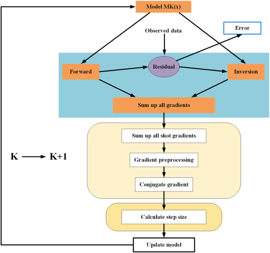
Figure 1. Workflow of the FWI method.

Results

Sub-sag model test

The sub-sag model as shown in Figure 2 is established to verify the effectiveness and robustness of the FWI method proposed in this paper based on Hessian operator pre-processing. The model size is 4000 m × 2000 m and the space grid spacing is 10 m. Riker wavelet with a center frequency of 25 Hz is selected to excite the seismic wave source, with a shot spacing of 40 m and a trace spacing of 20 m. A total of 100 shots are excited and 190 traces are received per shot. 20 layers CPML absorption boundary conditions are used at the model boundary, the sampling interval is 1 ms, and the recording time is 3 s. Figure 3 shows the 50^th shot field record excited by the forward simulation. By taking the gradient of the wave field propagated by seismic waves, it is found that the wave field gradient near the shot point and the receiver point is higher, and the gradient energy of shallow and deep wave field is significantly different (as shown in Figure 4A), and the difference of the gradient field affects the accuracy of FWI. Hessian matrix contains the information of gradient and amplitude, and gradient can be pre-processed by solving the inverse of the matrix. Based on this, Hessian operator preprocessing is used in this paper to improve the gradient value of the seismic wave field (as shown in Figure 4B). It can be seen that the gradient value of the wave field after Hessian operator pre-processing distributes evenly in shallow layer and deep layer.

Figure 2

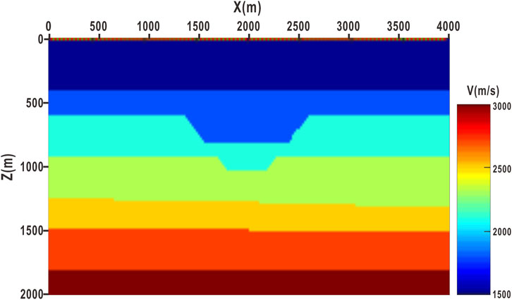
Figure 2. Sag velocity model and geometry.

Figure 3

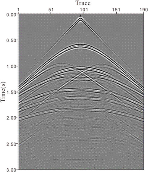
Figure 3. The 50^th shot record.

Figure 4

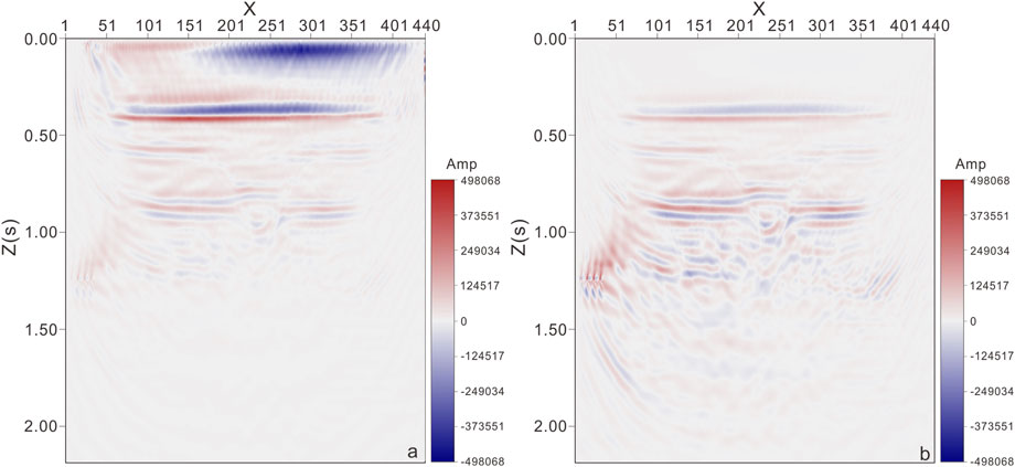
Figure 4. Amplitude gradient diagram before and after pre-processing (A) Before pre-processing, (B) After pre-processing).

FWI method is used to image the seismic wave field before and after the pre-processing, and inversion results are obtained as shown in Figure 5. Figure 5A is the velocity field of the real model, Figure 5B is the initial velocity model of FWI, Figure 5C is the inversion velocity field before the pre-processing, and Figure 5D is the inversion velocity field after the pre-processing. In Figure 5C, only the structures near the surface are reconstructed under the action of strong amplitude near the shot point, and the inversion of deep structures is not very effective. As can be seen from Figure 5D, the inversion accuracy has been greatly improved after preprocessing, compensating for the energy loss caused by amplitude attenuation in space, and obtaining good inversion results for both deep and shallow structures of the model.

Figure 5

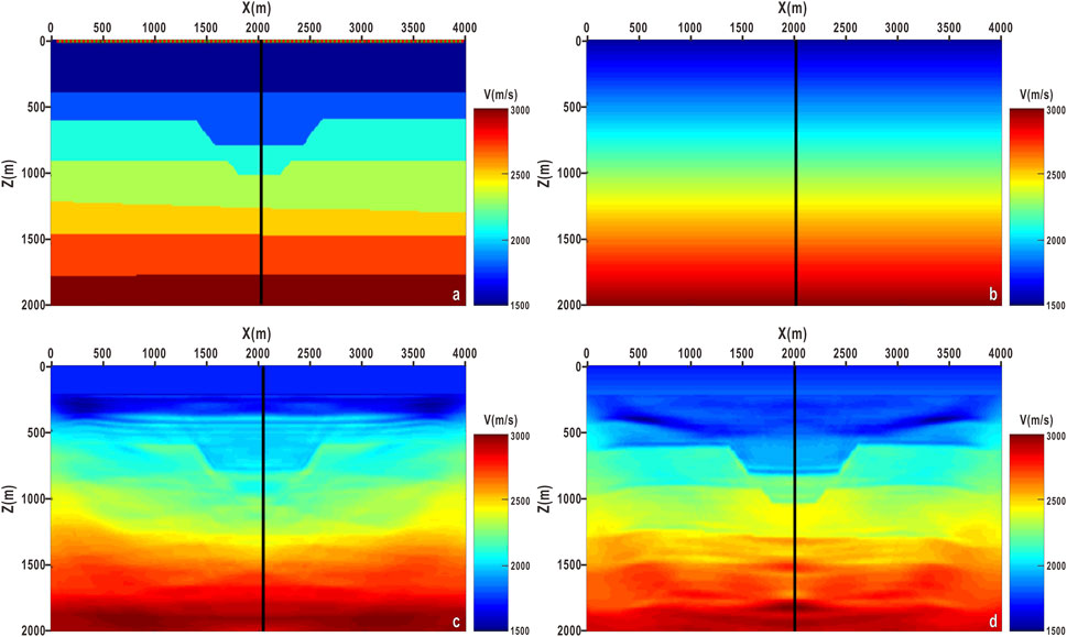
Figure 5. FWI results of before and after pre-processing (A). True velocity model, (B) Initial velocity model, (C) FWI result of before pre-processing, (D) FWI result of after pre-processing).

The seismic velocity at X = 2 km of the real model, the initial model, and the inversion results before and after the pre-processing are extracted respectively for comparative analysis, as shown in Figure 6. Figure 6A is the inversion velocity field before the pre-processing, Figure 6B is the inversion velocity field after the pre-processing, where the transverse represents the velocity and the vertical represents the depth. The pink line represents the velocity of the real model, the green line represents the velocity of the initial model, and the blue line represents the velocity of the inversion model. It can be seen from the figure that the inversion velocity curve after pre-processing is closer to the real velocity curve. Figure 7 shows the error analysis of the inversion velocity curve. The zeroing comparison between the initial velocity model and the inversion velocity model reflects the degree of fitting of the preprocessed model. The closer the value is to 0, the better the inversion result is. It can be seen from the figure that the fitting degree of the inversion results is improved after the application of pre-processing conditions.

Figure 6

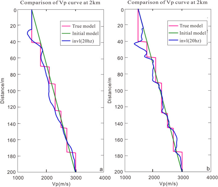
Figure 6. Comparison of single-trace velocity curves before and after pre-processing (A) Before pre-processing, (B) After pre-processing).

Figure 7

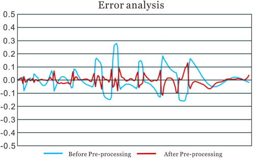
Figure 7. Error analysis before and after pre-processing.

Overthrust model test

The overthrust model (as shown in Figure 8) is used to verify the inversion effect of FWI on a complex model with drastic velocity changes. The model range is 20000 m × 4650 m and the mesh size is 25 m. The main frequency of excitation source is 10 Hz, the number of shots is 190. There are 384 traces per shot. The shot spacing is 200 m, and trace spacing is 50 m, sampling interval is 2 ms, recording length is 6 s. Figure 9 shows the single shot record of the 95^th shot in the forward numerical simulation of overthrust model. Figure 10 shows the gradient characteristics of the seismic wave field before and after pre-processing. It can be seen from the figure that the amplitude gradient of the seismic wave field is mainly distributed near the receiver point before pre-processing, and the deep energy is weak (as shown in Figure 10A). After pre-processing, the amplitude gradient of the seismic wave field becomes more uniform (as shown in Figure 10B).

Figure 8

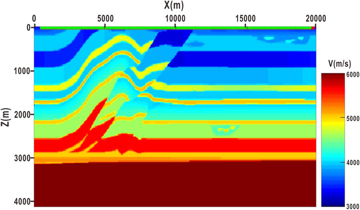
Figure 8. Overthrust velocity model and geometry.

Figure 9

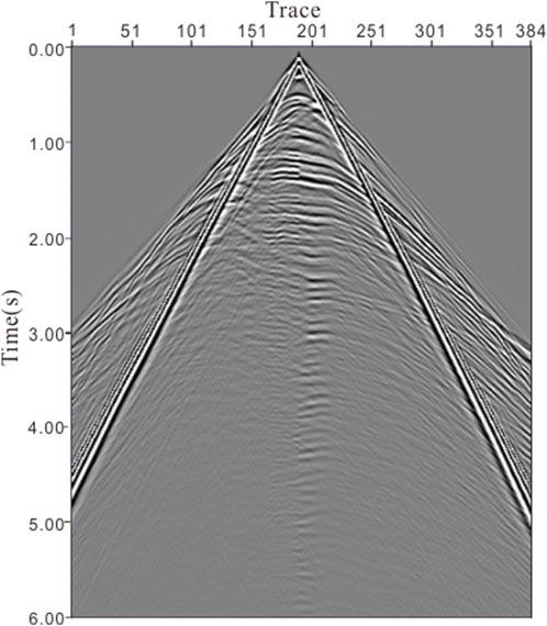
Figure 9. The 95^th shot record.

Figure 10

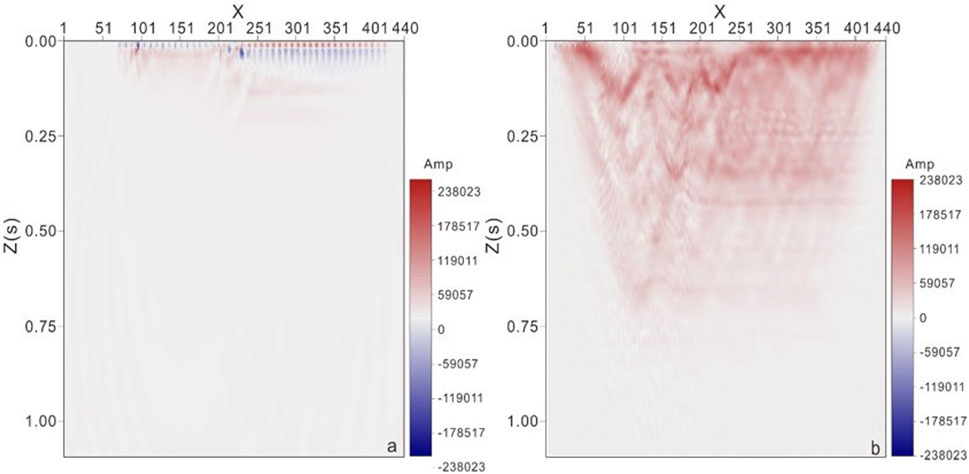
Figure 10. Amplitude gradient diagram before and after pre-processing (A) Before pre-processing, (B) After pre-processing).

Figure 11 shows the FWI results of the overthrust model before and after pre-processing. As can be seen from Figure 11C, before pre-processing, the basic shape of the model can be inverted, but the internal velocity features of the model are still different from the actual model. After pre-processing, the details of the inversion results are clearer, and the velocity features of Figure 11D are better matched with the actual model.

Figure 11

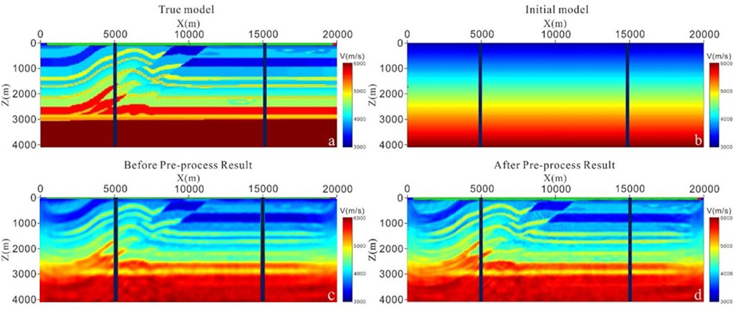
Figure 11. FWI results of before and after pre-processing (A). True velocity model, (B). Initial velocity model, (C). FWI result of before pre-processing, (D). FWI result of after pre-processing).

To quantitatively illustrate the effectiveness of the proposed method, considering that the overthrust model has a velocity change of the thrust fault structure, single-trace velocities at x = 5 km and x = 15 km in the horizontal direction were extracted from the actual model, initial model, and inversion model separately. Figures 12A, B are single-trace velocity curves before pre-processing, where the pink line is the real model velocity, the green line is the initial model velocity, and the blue line is the inversion model velocity. It can be seen that the inversion results before pre-processing are consistent with the actual velocity trend in morphology, but there are differences in internal details. Figures 12C, D are single-trace velocity curves after pre-processing. It can be seen that the inversion velocity curve is in good agreement with the real velocity, which effectively indicates that the inversion accuracy can be improved by pre-processing. Through comparative study, it is found that the FWI method by Hessian operator pre-processing has a great improvement on the internal detail imaging of complex structures, which further indicates that the FWI method can guide the velocity modeling of complex structures.

Figure 12

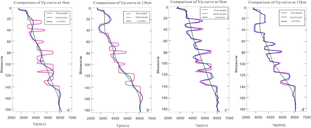
Figure 12. Comparison of single-trace velocity curves before and after pre-processing [(A) Before pre-processing at X = 5 km, (B) Before pre-processing at X = 15 km, (C) After pre-processing at X = 5 km, (D) After pre-processing at X = 15 km].

Discussion

By employing the full wave field information to restore the structural morphology and distribution characteristics of various elastic parameters in underground space, FWI can realize the high-precision and multi-parameter modeling of underground media. In this paper, the adjoint gradient method is optimized to improve the solving accuracy of strong nonlinear problems, and the diagonal element of Hessian operator is used to scale the gradient, so that the amplitude of the gradient is inversely proportional to the sensitivity of the synthesized data, and the imaging accuracy of the deep and weak reflection region is effectively enhanced. The experimental results of sub-sag model and overthrust model show that the Hessian operator pre-processing can effectively improve the amplitude gradient difference of seismic wave field and improve the accuracy of FWI.

This study only uses the Hessian operator to improve the amplitude gradient of seismic fields, making the energy in the anomalous regions more consistent. Meanwhile, only the diagonal elements of the Hessian operator are used to simplify the matrix solution. Over the past 4 decades, FWI has witnessed rapid development and has exerted a profound influence on both the scientific and industrial communities. Although its application to real seismic data faces certain challenges, FWI remains a cutting-edge technique for enhancing imaging accuracy and continues to merit sustained research and development. In the realm of deep seismic reflection data processing, FWI plays a pivotal role in improving the precision of subsurface imaging. Looking ahead, as data processing methods continue to advance, computational techniques evolve at a rapid pace, and our understanding deepens, FWI is poised to further empower humanity in exploring the subsurface, uncovering new oil reservoirs, and elucidating the structure of the deep crust.

Data availability statement

The raw data supporting the conclusions of this article will be made available by the authors, without undue reservation.

Author contributions

F-LY: Writing–original draft, Writing–review and editing, Supervision. H-LZ: Data curation, Writing–original draft. F-MY: Software, Writing–original draft, Methodology. LW: Software, Conceptualization, Writing–review and editing. Y-HZ: Resources, Data curation, Writing–review and editing.

Funding

The author(s) declare that financial support was received for the research, authorship, and/or publication of this article. This research work is funded by the Young Scientists Fund of the National Natural Science Foundation of China (42,304,135) and the scientific research project of Gansu Coal Geology Bureau (2023-07).

Conflict of interest

Authors F-MY and Y-HZ were employed by BGP Inc., CNPC. Author LW was employed by Tuha branch of China Petroleum Group Logging Co., Ltd.

The remaining authors declare that the research was conducted in the absence of any commercial or financial relationships that could be construed as a potential conflict of interest.

Generative AI statement

The author(s) declare that no Generative AI was used in the creation of this manuscript.

Publisher’s note

All claims expressed in this article are solely those of the authors and do not necessarily represent those of their affiliated organizations, or those of the publisher, the editors and the reviewers. Any product that may be evaluated in this article, or claim that may be made by its manufacturer, is not guaranteed or endorsed by the publisher.

References

Backus, G. E., and Gilbert, J. F. (1967). Numerical applications of a formalism for geophysical inverse problems. Geophys. J. Int. 13 (1-3), 247–276. doi:10.1111/j.1365-246x.1967.tb02159.x

CrossRef Full Text | Google Scholar

Bian, A.-fei, Wen-hui, Yu, and Hua-wei, Z. (2010). Research progress of full waveform inversion methods in frequency domain. Prog. Geophys. (in Chinese) 25 (3), 982–993. doi:10.3969/j.issn.1004-2903.2010.03.037

CrossRef Full Text | Google Scholar

Boonyasiriwat, C., Valasek, P., Routh, P., Cao, W., Schuster, G. T., and Macy, B. (2009). An efficient multiscale method for time-domain waveform tomography. Geophysics 74 (6), WCC59–WCC68. doi:10.1190/1.3151869

CrossRef Full Text | Google Scholar

Choi, Y., Min, D. J., and Shin, C. (2008). Frequency-domain elastic full waveform inversion using the new pseudo-Hessian matrix:Experience of elastic Marmousi-2 synthetic data. Bulletin of the Seismological Society of America 98 (5), 2402–2415. doi:10.1785/0120070179

CrossRef Full Text | Google Scholar

Fichtner, A., and Trampert, J. (2011). Hessian kernels of seismic data functionals based upon adjoint techniques. Geophysical Journal International 185 (2), 775–798. doi:10.1111/j.1365-246x.2011.04966.x

CrossRef Full Text | Google Scholar

Hu, B. T., Huang, C., Dong, L. G., and Zhang, J. M. (2023). A constant fractional Laplacian operator based viscoacoustic full waveform inversion for velocity and atenuation estimation. Chines J. Geophy. (in Chinese) 66 (5), 2123–2137. doi:10.6038/cjg2022P0891

CrossRef Full Text | Google Scholar

Jianping, H., Chao, C., and Liu, M. (2018). A hybrid multi-scale full waveform inversion method based on frequency-wavenumber filter and its implementation strategies. Journal of China University of Petroleum( Edition of Natural Science) 42 (02), 50–59. doi:10.3969/j.issn.1673-5005.2018.02.006

CrossRef Full Text | Google Scholar

Li, J., Liu, W., Liang, Y., Wu, J., and Li, Z. (2023). Time-domain full waveform inversion based on high-order amplitude information. Progress in Geophysics (in Chinese) 38 (4), 1603–1609. doi:10.6038/pg2023GG0129

CrossRef Full Text | Google Scholar

Li, S. L. (2023). Numerical simulation of complex attenuating media and full waveform inversion methods. Northeast Petroleum University. doi:10.26995/d.cnki.gdqsc.2023.000012

CrossRef Full Text | Google Scholar

Liu, Z., Tong, S., Fang, Y., and Jia, J. (2021). Full elastic waveform inversion in Laplace-Fourier domain based on time domain weighting. Oil Geophysical Prospecting 56 (2), 302∼312–331. doi:10.13810/j.cnki.issn.1000-7210.2021.02.012

CrossRef Full Text | Google Scholar

Lyu, C., Capdeville, Y., Al-Attar, D., and Zhao, L. (2021). Intrinsic non-uniqueness of the acoustic full waveform inverse problem. Geophysical Journal International 226 (2), 795–802. doi:10.1093/gji/ggab134

CrossRef Full Text | Google Scholar

Ma, Y., and Hale, D. (2011). A projected Hessian matrix for full waveform inversion. SEG Technical Program Expanded Abstracts, 2401–2405. doi:10.1190/1.3627691

CrossRef Full Text | Google Scholar

Ma, Y., Hale, D., Meng, Z., and Gong, B. (2010). Full waveform inversion with image-guided gradient. SEG Technical Program Expanded Abstracts, 1003–1007. doi:10.1190/1.3513016

CrossRef Full Text | Google Scholar

Shin, C., and Ho, C. Y. (2009). Waveform inversion in the laplace—fourier domain. Geophysical Journal International 177 (3), 1067–1079. doi:10.1111/j.1365-246x.2009.04102.x

CrossRef Full Text | Google Scholar

Shin, C., Jang, S., and Min, D. J. (2001). Improved amplitude preservation for prestack depth migration by inverse scattering theory. Geophysical Prospecting 49 (5), 592–606. doi:10.1046/j.1365-2478.2001.00279.x

CrossRef Full Text | Google Scholar

Sun, H., Zhang, J., Xue, Y., and Zhao, X. (2024). Seismic inversion based on fusion neural network for the joint estimation of acoustic impedance and porosity. IEEE Transactions on Geoscience and Remote Sensing 62, 1–10. doi:10.1109/TGRS.2024.3426563

CrossRef Full Text | Google Scholar

Tarantola, A. (1984). Inversion of seismic reflection data in the acoustic approximation. Geophysics 49 (8), 1259–1266. doi:10.1190/1.1441754

CrossRef Full Text | Google Scholar

Tarantola, A. (1986). A strategy for nonlinear elastic inversion of seismic reflection data. Geophysics 51 (10), 1893–1903. doi:10.1190/1.1442046

CrossRef Full Text | Google Scholar

Wang, Y., and Dong, L. G. (2015). Acoustic multi-parameter full waveform inversion for VTI media based on the truncated Newton method. Chinese Journal of Geophysics 58 (8), 2873–2885. doi:10.6038/cjg20150821

CrossRef Full Text | Google Scholar

Warner, M., Ratcliffe, A., Nangoo, T., Morgan, J., Umpleby, A., Shah, N., et al. (2013). Anisotropic 3D full-waveform inversion. Geophysics 78 (2), 59–80. doi:10.1190/geo2012-0338.1

CrossRef Full Text | Google Scholar

Xiang, Li (2017). Full-waveform inversion from compressively recovered updates. Geophysical Prospecting for Petroleum 56 (1), 20–25. doi:10.3969/j.issn.1000-1441.2017.01.002

CrossRef Full Text | Google Scholar

Xin, T., Huang, J., Xie, F., Zhou, B., and Lu, Z. (2020). Frequency-domain full waveform inversion without source wavelet based on data similarity. Oil Geophysical Prospecting 55 (2), 341–350. doi:10.13810/j.cnki.issn.1000-7210.2020.02.013

CrossRef Full Text | Google Scholar

Yang, W. -y., Wang, X. -w., Yong, X. -s., and Chen, Q. -y.(2013). The review of seismic Full waveform inversion method. Progress in Geophys. (in Chinese) 28(2), 0766–0776. doi:10.6038/pg20130225

CrossRef Full Text | Google Scholar

Zhang, P., Xing, Z. Z., and Hu, Y. (2019). Velocity construction using active and passive multi-component seismic data based on elastic full waveform inversion. Chinese J. Geophys. 62 (10), 3974–3987. (in Chinese). doi:10.6038/cjg2019M0421

CrossRef Full Text | Google Scholar

Zhang, W. S., Luo, J., and Teng, J. W. (2015). Frequency multiscale full-waveform velocity inverion. Chinese J. Geophys. (in Chinese) 58 (1), 216–228. doi:10.6038/cjg20150119

CrossRef Full Text | Google Scholar

Zhang, M., Wang, H., Ren, H., Feng, B., Sui, Z., and Wang, Y. (2014). Full waveform inversion on the CPU/GPU heterogeneous platform and its application analysis. Geophysical Prospecting for Petroleum 53 (04), 461–467. doi:10.3969/j.issn.1000-1441.2014.04.012

CrossRef Full Text | Google Scholar

Zhang, J., Wang, Z., Li, J., Ma, X., Li, B., and Zhang, K.(2024). Multi-scale full waveform inversion method based on gradient preprocessing. Progress in Geophysics (in Chinese) 39(3), 1111–1119. doi:10.6038/pg2024HH0539

CrossRef Full Text | Google Scholar