A LithoScanner logging data processing method and application applicable to shale oil formation

Lithology identification is crucial for understanding the characteristics of reservoirs, optimizing development plans, and enhancing development efficiency. For shale oil formations, the mineral composition is complex and the lithological combinations are diverse, which imposes limitations on conventional well logging interpretation for lithology identification.LithoScanner Logging is a method for quantifying mineral content; however, discrepancies persist between logging-derived mineral content and core experimental results in the actual exploration and development process. There are four main problems in LithoScanner Logging data processing: 1. Core data used to calibrate the dry weight of LithoScanner Logging elements are difficult to locate; 2. Changes in sedimentary environments and downhole geological conditions in different regions have a greater impact onthe instrument’s built-in sensitivity parameters; 3. The converted yields of some elements with low dry weight percentages are converted to dry weight curves, and the data are distorted not reflecting the real situation of the stratum; 4. The optimization algorithm exhibits poor applicability, lacks robust constraints, converges rapidly, and tends to trap in local optima. In response to the four questions above. First, rock matrix density is calculated using density and nuclear magnetic resonance (NMR) logging data, serving as the basis for depth normalization of core data; secondly, based on the oxide closure model, the offset and scaling factor are added to the calculation of the elemental dry weights, so as to obtain the optimal solution of the logged elemental dry weights; lastly, the elemental dry weights are combined with the differential evolution method, and the density profile and the sum of the mineral dry weights is used as the constraints, so as to carry out the inversion of the mineral dry weight is inverted.The results of mineral inversion have been well applied in different types of shale oil such as Daqing Gulong, Sichuan Liang Gaoshan, Xinjiang Mabei, etc. The mean absolute error between calculated mineral dry weights and core XRD experimental results is less than 5%.

1 Introduction

Shale oil reservoirs are characterized by rapid changes in lithology and physical properties, as well as strong non-homogeneity, and their strong non-homogeneity poses a great challenge to the identification of sweet spots and efficient development (Zhao et al., 2024). LithoScanner logging has the capability to directly identify formation elements and thereby determine lithology, which allows it to bypass the influence of formation physical properties and oil content. However, when applied to shale oil formations, LithoScanner logging still encounters four major challenges: (1) It is challenging to accurately position the core data used for calibrating the elemental dry weights in rock scanning. (2) The significant variability in sedimentary environments and downhole geological conditions across different regions has a considerable impact on the instrument’s built-in sensitivity parameters. Using the default elemental sensitivity settings of the instrument is inappropriate. (3) Based on the principles of the Schlumberger rock scanning logging tool, the relationship between elemental yield and elemental dry weight is nearly linear. However, this simple linear relationship can lead to overfitting when converting the yields of certain elements with low dry weight proportions into dry weight curves, resulting in distorted data that fails to reflect the true formation characteristics. (4) After calibrating the elemental dry weights, it is necessary to interpret the dry weight proportions of formation minerals using the oxygen closure model. Typically, an optimization algorithm is employed to calculate mineral dry weights. However, the lack of robust constraints often leads to rapid convergence into local optima. This results in a narrow range of variation in the mineral profile solutions, which compromises the reliability of the interpreted mineral profiles. Consequently, the match between the interpreted mineral profiles and logging curves is poor, and the geological significance is limited.

For shale oil reservoirs, the application of stratigraphic elemental logging techniques combined with supporting core experiments is the main technical approach for continuous characterization of shale oil lithological profiles (Liao, 2015). LithoScanner logging is currently used to identify the lithology of the formation, through the Schlumberger LithoScanner logging, through the emission of fast neutrons into the formation, and measure the gamma-ray spectrum of the reaction between the fast neutrons and the nuclei in the formation, in order to calculate the production of each element, and then calculate the dry weight of each element, for the traditional elemental logging technology, the identification of the elemental species and the accuracy of a greater improvement (van den ord, 1991; Cannon and Coates, 1990). In terms of the interpretive application of this technology, Gainitdinov et al. (2024) from abroad improved the method of calculating the dry weight of minerals from LithoScanner logging elemental dry weights by utilizing a variety of machine learning algorithms; Lai et al. (2022) used LithoScanner logging data combined with conventional logging data to evaluate the lithology and brittleness of shale oil reservoirs and summarized the relationship between lithology, brittleness, and oil content in unconventional reservoirs; Zhang et al. (2024) utilized LithoScanner logging and accurately calculated the mineral content based on a decision tree model, and combined it with 2D NMR logging to comprehensively evaluate the lithology, effective porosity, and fluid properties of shale oil reservoirs. In China, Adeoti et al. (2019) utilized LithoScanner logging technology, combined with the least squares method and generalized inverse matrix solution, proposed corresponding data processing methods, and made significant progress in the interpretation of complex lithological formations in various oilfields; Waters et al. (2020) applied LithoScanner logging to formations with a variety of lithologies and accurately measured the content of clay, silica, and calcium in the formations. Based on the previous research, this paper explores four problems in the data processing and interpretation process in depth, and innovatively utilizes core XRD experiments to calculate core dry weight density to calibrate LithoScanner logging processing data. The pre-processing process of elemental yield and core elemental dry weight is also established to increase data stability. Based on the differential evolution method with good applicability, it is proposed to add the data processing and interpretation process based on the constraints of fusing multiple logging data such as conventional density profiles and nuclear magnetic logging, and improving the optimization algorithm, The interpretation results can be applied to the continuous characterization of lithological profiles of multiple types of shale oils, and the analysis of the coupled relationship between lithological assemblage characteristics and production was implemented using the Daqing Gulong shale oil as an example, which verified the reliability of the data processing flow and interpretation method.

2 LithoScanner logging principle and common processing flow

Stratigraphic elemental capture spectroscopy originated in the 1980s, initially using pulsed neutron generator (PNG)-based cable tools and thallium-doped sodium iodine (NaI(Tl)) scintillation detectors (Juntao et al., 2018). The basic principle of its work is based on the instrument pulse seed generator, which produces gamma rays generated by the interaction of fast neutrons with stratum rocks, see Figure 1, and obtains inelastic scattering gamma spectra and thermal neutron capture gamma spectra by means of detectors and spectral analysis, thus obtaining information on the elements of the stratum (Craddock et al., 2013). Subsequent instruments in the field of gamma scintillation detector materials continue to push the boundaries of innovation, the main development in recent years is the development of a pulsed neutron generator by adjusting the timing, effectively distinguish between inelastic scattering spectra and thermal neutron capture spectrum LithoScanner logging instrument, can significantly improve the identification of the types of elements in the stratigraphy and accuracy, in particular Mg, C and other more critical elements (Galford et al., 2009; Mao et al., 2022; Lai et al., 2024), This is significant for the quantitative identification of minerals in shale oil formations with diverse mineralogical species.

Figure 1

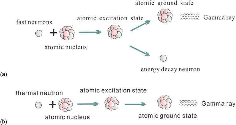
Figure 1. The two primary mechanisms of neutron interaction with atoms in the formation (A) Schematic diagram of inelastic scattering of neutrons(Neutron inelastic scattering refers to the process where high-energy neutrons collide with atomic nuclei, losing some of their energy and exciting the nuclei to higher energy levels. The nuclei then release gamma rays as they return to their ground state. This process can be used to detect the elemental composition of formations) (B) Schematic diagram of thermal neutron capture(Thermal neutron capture refers to the process where thermal neutrons (low-energy neutrons) are absorbed by atomic nuclei, causing the nuclei to become unstable and release gamma rays. The energy characteristics of these gamma rays can be used to identify elements in the formation).

The instrument consists of three main modules: a neutron generator, a shielding section (which shields the neutrons and gamma rays directly from the generator), and a gamma ray detector (Figure 2). The main working principle is that the pulsed neutron generator emits neutrons with an energy of 14-MeV into the stratum (Yang and Wang, 2012; Radtke et al., 2012), and these neutrons interact with the stratum to produce gamma rays. By choosing a suitable neutron pulse sequence (Figure 3), the inelastic scattering energy spectrum associated with the gamma ray count rate (SBUR-α*SEAR) and the thermal neutron capture spectrum can be obtained through the detection by the scintillation detector and the processing of photomultiplier tube (SEAR + SLAT + STAU-β*SBKG), while a shield-containing instrument is wrapped around the enclosure near the detector to minimize the effect of captured gamma rays from the instrument on the detector. At this time, the energy spectrum can be regarded as a linear superposition of the standard spectra of each element in the stratum, and the yield that can characterize the relative content of each element can be obtained after deconvolution of the spectrum (Craddock et al., 2013), and the sum of the relative yields of each element is 1. The relative yield of each element depends on the abundance of the elements in the stratum as well as the instrument’s sensitivity to each element.

Figure 2

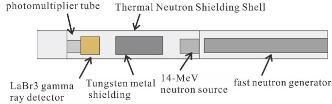
Figure 2. LithoScanner Instrument Measurement Section (The tungsten metal shell can effectively reduce the impact of captured gamma rays from the instrument on the detector).

Figure 3

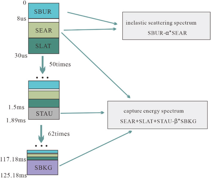
Figure 3. Neutron pulse time series (An appropriate timing sequence of the pulsed neutron generator can help effectively distinguish between the inelastic scattering spectrum and the capture energy spectrum).

Elemental relative yields to mineral dry weight, the Schlumberger treatment process is divided into two main steps, S1 and S2 (Figure 4). The first is S1:LithoScanner logging relative yield to formation elemental dry weight conversion. The principle is based on the oxygen closure model, which connotes that the weight of each mineral in the formation sums to 1, and the weight of its oxide form sums to 1. Schlumberger has a set of mineral model libraries with sensitivity S for each element. By constructing oxygen closure models for the major elements of the formation, the dry weights of each element can be derived through a built-in iterative inversion algorithm (Sun et al., 2014).

$W_i=F*Y_i*S_i(1)$

where: Wi is the dry weight of an element in the formation; Y_i is the relative yield of an element; F is the formation normalization factor; Si is the sensitivity of an element.

Figure 4

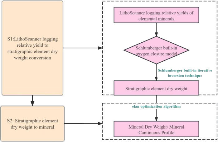
Figure 4. Schlumberger Interpretation Flowchart (This interpretation process represents the currently standard workflow, which involves converting the elemental yields detected by the instrument into the dry weights of formation elements, followed by further processing to derive the dry weights of minerals).

And then comes the S2 step: the transformation process from formation elemental dry weight to mineral profile. It is necessary to establish a multidimensional equation between elemental dry weight and formation mineral dry weight based on the specific gravity of elements in the oxygen closure model (Herron and Herron, 2000; Herron et al., 2002), see Equation 2, and the formation mineral dry weight, i.e., the continuous profile of formation minerals, can be solved by the built-in ELAN optimization algorithm. In order to obtain a continuous lithology and lithofacies profile, a ternary division map of mineral weight components can be constructed to identify the lithology and lithofacies based on the geological characteristics of the study area.

$\left\{\begin{array}{l}{W}_{Mg}=\sum \left(w_{\text{Percentage}\text{of}Mg}*w_{\text{Dry}\text{weight}\text{of}\text{minerals}\text{containing}Mg}\right)\\ •••\\ •••\\ •••\\ W_{S\mathrm{i}}=\sum \left(w_{\text{Percentage}\text{of}S\mathrm{i}}*w_{\text{Dry}\text{weight}\text{of}\text{minerals}\text{containing}S\mathrm{i}}\right)\end{array}\right.(2)$

where: W_Si is the dry weight of elemental Si; w_{Percentage of Si} is the weight percentage of a mineral containing elemental Si; w_{Dry weight of minerals containing Si} is the proportion of elemental Si in the mineral.

3 Problems in the interpretation

In this paper, starting from the actual interpretation process, the petrographic scanning interpretation process disclosed by Schlumberger mainly has the following problems, see Figure 5: Firstly, considering that the depositional environments of foreign marine shale oil and domestic land-phase shale oil are different, see Table 1, the environments differ in temperature, pressure, salinity, acidity, alkalinity, redox conditions, etc., which will affect the formation and preservation of the minerals, and therefore the mineral species and mineral distribution forms will be different; at the same time, the downhole formation conditions, formation gradient, borehole conditions, etc., will also be different. At the same time, the downhole stratigraphic conditions, stratigraphic gradient, borehole conditions, etc., will also be different, and the difference of the downhole environment will affect the sensitivity of the instrument to the detection of stratigraphic elements, and its parameters (Zhang and Li, 2022; Miles and Badry, 2014) (generally non-adjustable), and it is inappropriate to directly apply the built-in oxygen closure model of Schlumberger to calculate the stratigraphic elements of the dry weight. In addition, the shale oil depositional environments in different regions of China are also different from each other as shown in Table 2, so the relative yield to the elemental dry weight needs to be corrected based on the actual mineral dry weight of the formation.

Figure 5

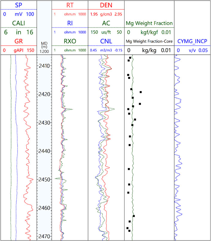
Figure 5. Interpretation Results of Magnesium Dry Weight Using Schlumberger’s Method (The second channel on the left represents the experimental measurement points of the magnesium element and its dry weight curve. The coupling relationship between the two is quite poor. The amplitude of change in the dry weight curve is extremely small, nearly presenting as a straight line. However, the amplitude of change in the relative yield curve in the first channel on the left, which reflects the real - world conditions of the formation, is quite large).

Table 1

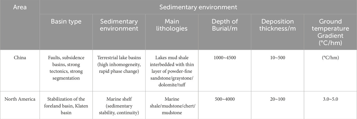
Table 1. Statistics of North American and domestic shale oil depositional environments.

Table 2

Table 2. Statistics of domestic shale oil deposition environments.

Secondly, the iterative inversion algorithm of Schlumberger’s relative production into the dry weight of formation elements is unknown, and the oxygen closure model and sensitivity are set by default. For shale oil formations with diverse mineral types, the built-in module of Schlumberger has poor adjustability, and at the same time the dry weight accounts for a relatively low percentage of the elements, which is prone to overfitting of the data, and fails to respond to the real situation of the formation; As shown in Figure 5, the second channel on the left is the experimental measurement point of magnesium element and the dry weight curve, the coupling relationship between the two is very poor, and the variation of dry weight curve is very small, almost a straight line, but the variation of relative yield curve which reflects the real situation of the formation is very large, which indicates that the solved dry weight curve of magnesium element does not reflect the complex mineral changes in the longitudinal direction of shale oil formation, and magnesium element, as a landmark constituent of the dolomite of shale oil formation, can more intuitively reflect the changes of dolomite content of formation, so such problems need to be solved. As the signature element of dolomite in shale oil formation, the dry weight content of magnesium can reflect the change of dolomite content in the formation more intuitively, so the solution of this kind of problem is very necessary.

Thirdly, the optimization algorithm for calculating the dry weight of minerals based on the dry weight of the formation is unknown, if the least squares optimization algorithm commonly used in the system of linear equations is used, it is easy to fall into the local optimal solution, and the range of variation of the solution value domain is small, and the shale oil formation tends to have a strong non-homogeneity in the longitudinal direction, and the minerals change continuously and quickly, and it is difficult to react to the actual situation of the formation in the optimal solution of such an algorithm (Mosse et al., 2014). At the same time, because of the large uncertainty in the solution process, if there is a lack of better constraints to optimize the objective function, the optimal solution is less coupled with the logging data reflecting other geophysical characteristics of the stratum, which is difficult to provide geologists with effective information and lacks geological significance; for example, in Figure 6, the first channel on the right hand side is the mineral profile obtained from the treatment, and the optimal solution of various minerals in terms of dry weight has no change because of the too-fast convergence, and is poorly coupled with the conventional The coupling relationship with the conventional logging curve is poor, and the reference significance is small.

Figure 6

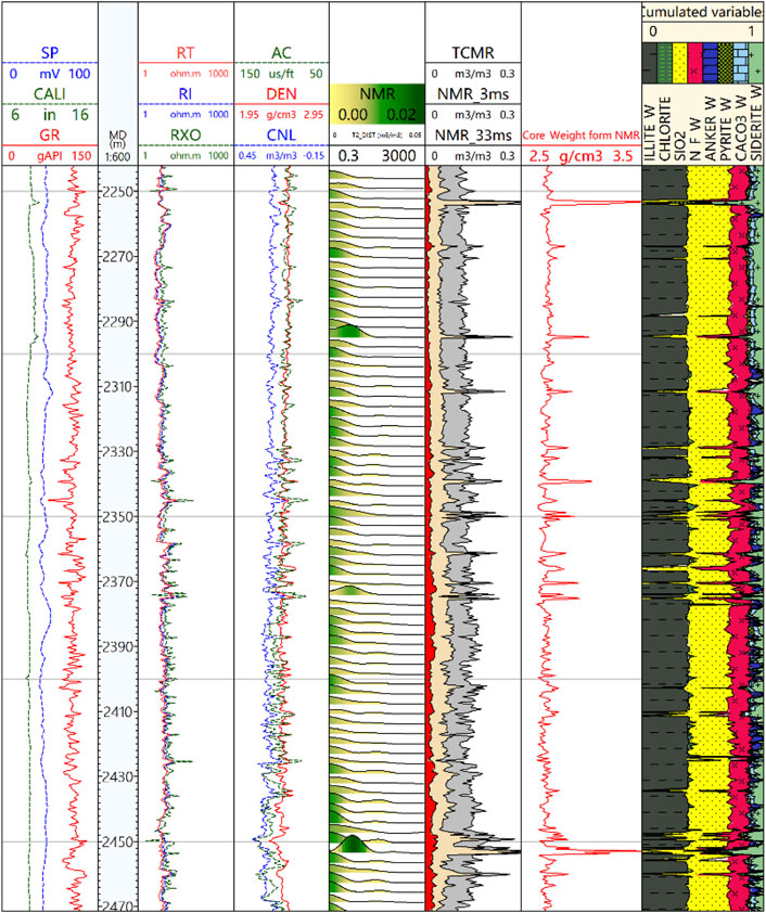
Figure 6. Processing results of a well after using the least squares optimization algorithm (It can be seen from the first mineral profile on the left that the dry weight content of each mineral has not changed significantly. This indicates that this algorithm has difficulty reflecting the actual situation of the shale - oil formation).

Fourthly, core XRD experimental mineral dry weight directly calibrated mineral dry weight profile is inappropriate, first of all, the core XRD experiments should be done to normalize the processing, there’s no better way to put it back in place, and secondly, the results of the mineral profile processing is still uncertain, the use of the core XRD experiments directly calibrated there will be a large error (Herron et al., 2014), the core experimental data is larger, normalization is also more difficult. Finally, common problems existing in the processing of the general processing flow are summarized, as shown in Figure 7.

Figure 7

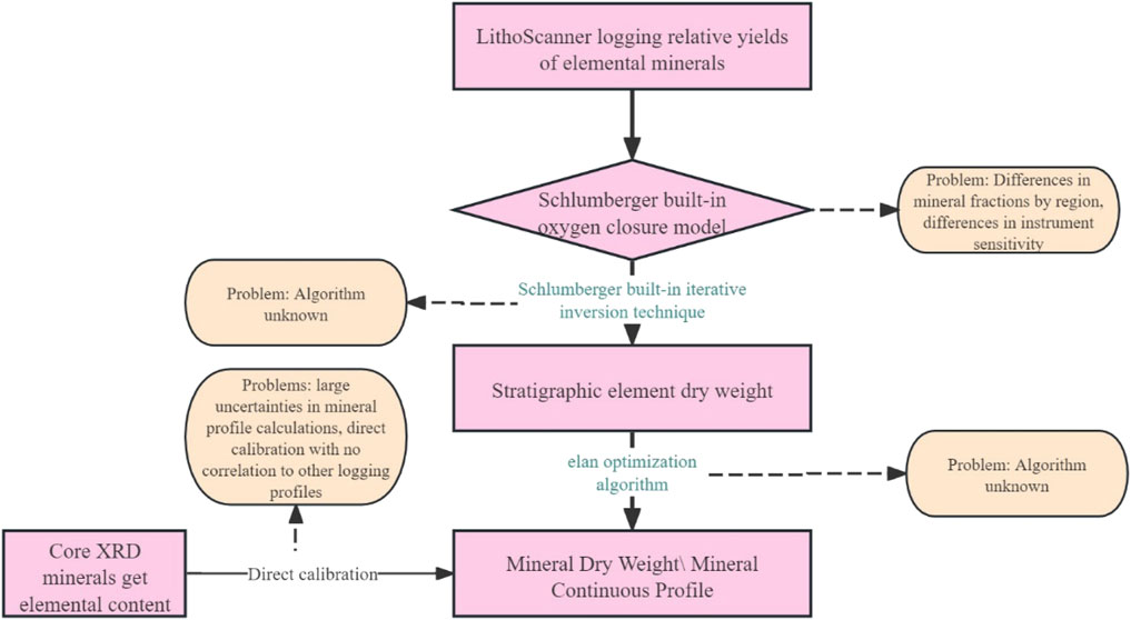
Figure 7. Interpretation flow of lithology scan processing.

4 LithoScanner logging data processing methods and procedures

In view of the many problems in the above processing process, the data processing process was improved on the basis of previous research, and solutions were proposed for the corresponding problems, see Figure 8.

Figure 8

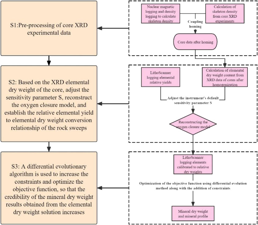
Figure 8. Interpretation flow of modified lithology scan processing (added the S1 data preprocessing step and improved the S2 and S3 processing workflows. The improved workflows correspond to the S1 and S2 steps in the standard processing workflow, respectively).

The whole process is divided into three parts, S1: Firstly, for the normalization of core XRD experimental data, the total porosity of NMR logs and conventional log density curves can be used to back-calculate the density of the rock skeleton, The dry weight density of the experimental site was also calculated based on the XRD mineral dry weight of the core; Deep normalization of core XRD dry weight density using rock skeleton density as a reference, thus completing the normalization of core XRD experimental data, Figure 9 shows the comparison of the effect of a well before and after homing, and the right data point is better coupled with the NMR-calculated skeleton density curve after homing upward by 1.9 m.

Figure 9

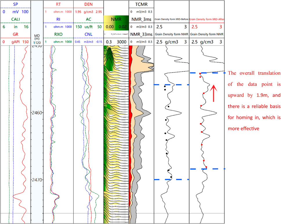
Figure 9. Graphs of the results of core XRD experimental data before and after positioning (Judging from the homing results, the added step S1 can effectively solve the problem of homing core XRD experimental data).

Inversion of rock skeleton density using NMR total porosity and conventional logging density curves, specifically:

${\rho }_{\text{ma}}=\frac{{\varphi }_{HC}-\rho }{{\varphi }_{HC}-1}(3)$

where: ${\rho }_{\text{ma}}$ is the calculation of rock skeleton density based on logging volume model and NM total porosity; ${\varphi }_{HC}$ is NMR total porosity.

Calculate the dry weight density of the experimental site, specifically:

${\rho }_{\mathrm{x}-\text{ma}}=1/\left(\sum \frac{W_{\text{dry}\text{weight}\text{of}\text{minerals}}}{{\rho }_{\text{mineral}\text{density}}}\right)(4)$

where: ${\rho }_{\mathrm{x}-\text{ma}}$ is the dry weight density of the core calculated based on XRD; W_{dry weight of minerals} is the mass fraction of each mineral in the core XRD; ${\rho }_{\text{mineral}\text{density}}$ is the mineral density.

Step S2 Considering the influence of different geological environments in each region on the downhole measurement instrument, using the elemental dry weight calculated after the core XRD experiment homing as the standard, and based on the principle of the oxygen closure model, an offset offset is added for correcting the instrument’s sensitivity to the formation elements S, see Equation 2, to establish the relationship between the relative yield of rock-sweeping elements and the elemental dry weight conversion.

$W_{\text{dry}\text{weight}\text{of}\text{an}\text{element}}+\text{offset}=\frac{P_{\text{Elemental}\text{yield}}}{S}(5)$

For elements with a relatively low percentage of dry weight, it is easy to overfit the data, The relative yields of core element dry weights and LithoScanner logging elements were standardized to ensure zero mean and unit variance and to improve data stability, At the same time, A regularization term is introduced to optimize the objective function. By tuning hyperparameters (α and λ), optimal scaling and translation factors are derived, and find the optimal translation factor offset and the optimal scaling factor S, so as to get the optimal logging element dry weight solution, and the flowchart is shown in Figure 10:

Figure 10

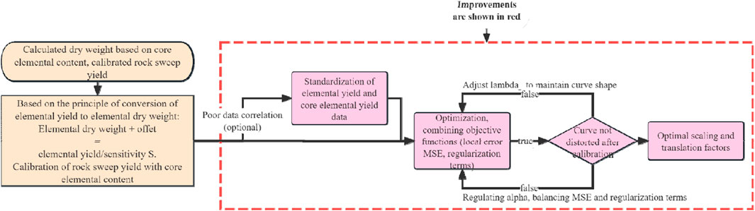
Figure 10. LithoScanner logging elemental relative yield - core elemental dry weight conversion flowchart (The improved part of the process is within the red box. Optimizing the objective function with the regularization term can significantly enhance data stability).

Assuming that there are i core samples, in terms of elemental magnesium, for each sample of the core there is a corresponding dry weight mass fraction W(Mg) elemental dry weight and LithoScanner logging in terms of elemental Mg yield P_{Mg yield}. According to the given relation Equation 5, a system of equations containing i equations can be created see Equation 6, and the objective function of the least squares method can be written, see Equation 7, and the regularization term can be introduced to optimize the objective function, see Equation 8.

$\left\{\begin{array}{l}{\mathrm{P}}_1=S_1*\left(W_1+offset\right)\\ {\mathrm{P}}_2=S_2*\left(W_2+offset\right)\\ {\mathrm{P}}_3=S_3*\left(W_3+offset\right)\\ ⋮\\ {\mathrm{P}}_i=S*\left(W_i+offset\right)\end{array}\right.(6)$

${\displaystyle \sum _{\mathrm{j}=1}^{\mathrm{i}}}{\left(P_j-S*\left(W_j+offset\right)\right)}^2(7)$

The objective function after introducing the regularization term:

${\displaystyle {\sum }_{j=1}^i}\left(a*{\left(P_j-S_i*\left(W_j+{offset}_i\right)\right)}^2+\lambda *\left(S_i^2+{offset}^2\right)\right)(8)$

The processing results are shown in Figure 11, taking magnesium and sulfur as examples, the third channel on the right side is the processing results of sulfur, the green solid line is the dry weight of sulfur before improvement, the blue solid line is the dry weight of sulfur after improvement, the red solid point is the dry weight of core experiment, the fourth channel on the right side is the processing results of magnesium, the second channel on the right side is the LithoScanner logging relative yield curve of magnesium, and the first channel on the right side is the LithoScanner logging relative yield curve of sulfur. It can be seen that before and after the improvement, the compliance rate of Mg and sulfur elements with low dry weight ratio with the experimental points is greatly improved, and the morphology with the relative yield curve of the elements is closer to each other, so that the stratigraphic information detected by LithoScanner logging can be retained to a greater extent.After applying this process, the processing results of a single well in the Gulong area are shown in Figure 12.

Figure 11

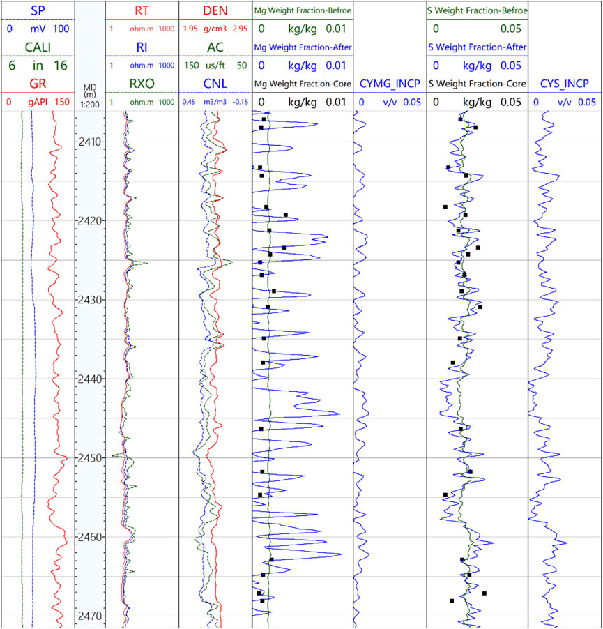
Figure 11. Comparison of elemental dry weight and core elemental dry weight before and after the improvement of Mg and sulfur elements (Before and after the improvement, the coincidence rate of magnesium and sulfur elements, which have a relatively low dry weight proportion, with the experimental points has increased significantly. Their shapes have also become closer to those of the relative yield curves of the elements. As a result, more of the formation information detected by the LithoScanner logging can be retained).

Figure 12

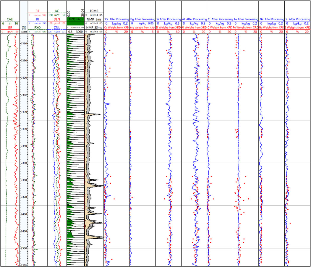
Figure 12. LithoScanner logging processed dry weights for each element of the formation compared to the elemental dry weights calculated from the core experiments (The final results of each element of the formation according to this process are shown in Figure 14, in which the blue curves of the right lane 2∼lane 9 are the results of dry weight processing of elemental content of LithoScanner logging of a well, and the red points are the results of XRD calculation of the rock core).

Step S3, the transformation of elemental dry weight to mineral dry weight, Schlumberger uses the optimization algorithm is unknown, the adjustability is poor, according to the obtained elements to find the optimal translation factor offset and the optimal scaling factor S, can be obtained after the transformation of the elemental yield of the elemental dry weight curves, see Figure 14 (based on the elemental content of the core to calibrate the LithoScanner logging after the elemental dry weights), and then can be used to these dry weights curves can be used to solve for mineral dry weights. Schlumberger’s oxygen closure model is constructed assuming that the sum of the weights of the minerals in the formation is one, the sum of the dry weights of the oxides is one, and the sum of the weights of the elements is one. Assuming that the main minerals in a region are quartz, sodium feldspar, calcite, illite, and chlorite, the expression of the region can be seen in Equations 9–11:

${\left(\text{Quartz}+\mathrm{N}-\text{Feldspar}+\text{Calcite}+\text{Illite}+\text{Chlorite}\right)}_{\text{weights}}=1(9)$

${\left({\text{Sio}}_2+{\text{Na}}_2\mathrm{O}+{\text{Al}}_2{\mathrm{O}}_3+\text{CaO}+\text{MgO}+\text{FeO}+{\text{CO}}_2\right)}_{\text{weights}}=1(10)$

${\left(\text{Si}+\mathrm{N}\mathrm{a}+\text{Al}+\text{Ca}+\text{Fe}+\text{Mg}+\mathrm{C}+\mathrm{O}\right)}_{\text{weights}}=1(11)$

Again using the element magnesium as an example, there is:

$W_{MG}=\sum W_{\text{percentage}\text{of}\text{Mg}}*W_{\text{Dry}\text{weight}\text{of}\text{minerals}\text{containing}\text{Mg}}(12)$

For this region, there are 8 elements and 5 minerals, which is equivalent to establishing a system of equations with 8 dimensions and 5 unknowns. Schlumberger’s procedure on optimization algorithms is unknown, and the optimization algorithm of least squares is used to calculate the dry weight of minerals, with the following objective function:

$\min \left({\sum \left(W_{\text{optimum}\text{element}\text{dry}\text{weight}}-W_{\text{elemental}\text{yield}\text{to}\text{elemental}\text{dry}\text{weight}}\right)}^2\right)$

There are two problems with this approach: first, the least squares algorithm converges faster, easily falls into the local optimal solution, and the range of variation of the mineral profile solution is smaller, whereas shale oil formations tend to be more inhomogeneous and the mineral continuum changes faster; Secondly, it lacks better constraints, and the interpreted mineral profiles have low credibility and low coupling with logging curves, which is difficult to provide reference value for geologists and has no better geological significance. To reconstruct the oxygen closure model for this purpose, the following improvements were made: first, two constraints were added: 1) the skeleton density profile obtained from the mineral dry weight calculation was coupled with the logging calculation skeleton density profile; 2) the sum of the mineral dry weights was 1. And it is incorporated into the optimized objective function and given different weights weight1, weight2, which makes the interpreted profiles match well with the logging curves, increase the credibility, and at the same time have better geological significance; Secondly, the differential evolution algorithm with the advantages of global optimization is used to obtain the optimal mineral profiles. The two constraints, when added to the objective function, become:

Constraint 1:

$penalty1=weight1*\left(1/\sum \left(W_{\text{mineral}\text{mass}\text{fraction}}/{\rho }_{\text{mineral}\text{density}}\right)-{\rho }_{\text{NMR}\text{Skeleton}\text{Density}}\right)(13)$

Constraint 2:

$penalty2=weight2*\sum \left(W_{\text{mineral}\text{mass}\text{fraction}}-1\right)(14)$

where: weight1 is the weight constant; W_{mineral mass fraction} is the calculated mass fraction of each mineral; ρ_{mineral density} is the corresponding density of the mineral; ρ_{NMR skeleton density} is the skeleton density.

Calculated from the density curves of NMR and conventional logging, weight2 is the weight constant, constraint1 that is, for the skeleton density curve calculated from the dry weight of the mineral coupled with the skeleton density curve of the logging calculation to do constraints, and constraint2 that is, for the dry weight of the minerals to do constraints on the sum of the 1 The constraint 2 is the constraint that the sum of mineral dry weights is 1.

Optimized objective function:

$\begin{array}{ll}\hfill & \min \left(\left({\sum \left(W_{\text{optimum}\text{element}\text{dry}\text{weight}}-W_{\text{elemental}\text{yield}\text{to}\text{elemental}\text{dry}\text{weight}}\right)}^2\right)\right.\hfill \\ \hfill & \left.+|\text{Constraint\hspace{0.17em}}|1|+|\text{Constraint\hspace{0.17em}}|2\right)\hfill \end{array}(15)$

The objective function is calculated using differential evolution method. The main calculation process of differential evolution method is to generate an initial population randomly within the constraints, use two random vectors in the population to subtract, produce the difference vector of two vectors, add the difference vector to the third vector to produce a new variant vector, and cross with the target vector to produce the experimental vector, and compare the fitness of the experimental vector with the target vector, select the appropriate vector for the next round of calculation, and finally output the optimal solution through continuous iterative calculations. Compare the fitness of the experimental vector with the target vector, select the appropriate vector for the next round of computation, and finally output the optimal solution through continuous iterative computation.

In this paper, the differential evolution method adopts Equations 13, 14 as constraints and Equation 15 as the objective function.

(1) Generate an initial population POP(0) with initial population POP(0) = {X₁ (0),…,X_j (0),…,X_n (0)}, and let there be M species of major minerals in the region, then X_j (0) is an M-dimensional vector.

(2) Randomly select the target vector X_i (0) to generate the variation vector:

$\left.{\mathrm{V}}_i\left(1\right)={\mathrm{X}}_i\left(0)+\mathrm{F}(X_{r1}\left(0\right)-{\mathrm{X}}_{r2}\left(0\right)\right.\right)(16)$

where, r1,r2 are randomly selected mutually different indices from {1.2, … n} and F is the difference weight.

(3) Cross the variant vector with the target vector to generate the experimental vector Ui(1), where the cross rule for each mineral stem weight j is as follows:

$U_{ij}\left(1\right)=\left\{\begin{array}{l}{V}_{ij}\left(1\right),\begin{array}{ccc}\mathit{ran}{d}_{ij}\le CR& or& j=rand\left(j\right)\end{array}\\ X_{ij}\left(0\right),else\end{array}\right\}(17)$

where rand_ij is a random number in the range [0,1]; CR is the crossover probability; rand (j) ensures that at least one of the dimensions comes from the variation vector.

(4) Substitute the experimental and target vectors into the objective function Equation 15 for computation and select either the experimental or target vector into the next-generation.

$X_i\left(1\right)=\left\{\begin{array}{l}{U}_i\left(1\right),f\left(U_i\left(1\right)\right)\le f\left(X_i\left(0\right)\right)\\ X_i\left(0\right),f\left(U_i\left(1\right)\right)>f\left(X_i\left(0\right)\right)\end{array}\right\}(18)$

The vectors entering the next-generation form the population of the second generation and repeat this step, comparing the size of the average value of the population fitness of two consecutive generations with the error threshold, and terminating the procedure when the average value of the fitness is less than the threshold, at which point the optimal solution can be obtained. Interpretation results are shown in Figure 13, the right lane 2∼lane 9 is LithoScanner logging calculated mineral dry weight, the pink point in the lane is the core calculated mineral dry weight, the coincidence is better, the second lane on the right side is the interpretation of the mineral profile, the 10th lane on the right side is the inverse calculation of the skeleton density according to the solution of the mineral profile in red, and the black line is the NMR calculation of the skeleton density, and the effect of the two couplings is better due to the use of constraints.Meanwhile, the absolute errors before and after the statistical homing and before and after the method improvement are shown in Figure 14, and the method improvement is within 5%, and the conformity rate has been greatly improved, which has a better application effect.

Figure 13

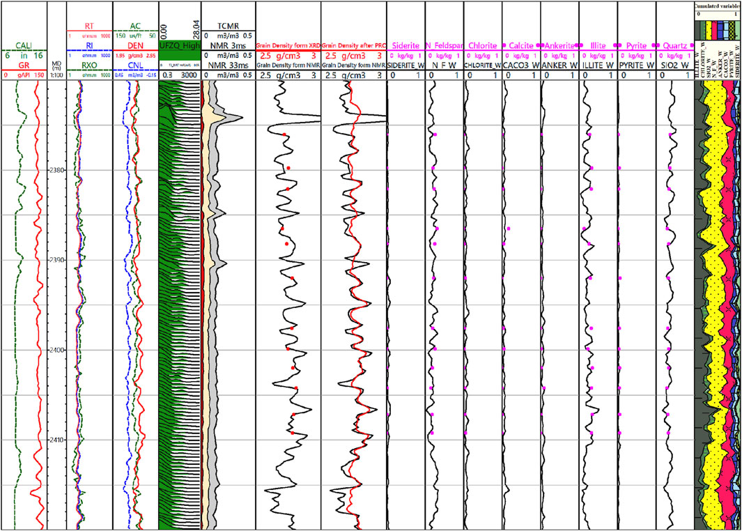
Figure 13. Mineral profile interpretation results of a well with improved process (Lanes 2 - 9 on the right represent the dry weight of minerals calculated by LithoScanner logging. The pink dots in these lanes are the dry weight of minerals calculated from the core, showing a good match. The second lane on the right is the interpreted mineral profile. The red curve in the 10th lane on the right is the skeleton density calculated inversely from the solved mineral profile, and the black line is the skeleton density calculated by nuclear magnetic resonance. Due to the adoption of constraint conditions, the coupling effect between the two is quite good).

Figure 14

Figure 14. Histogram of absolute error statistics before and after improvement (After processing with this method, the absolute error with the core XRD experiment data after homing is controlled within 5%, resulting in a significant improvement in interpretation accuracy).

5 Application examples

The technological process was implemented in three different blocks of Gulong Qingshankou Formation (mud-type shale oil) in Songliao Basin, Liang Gaoshan Formation (mud-type shale oil) in Sichuan Basin, and Mabei Fengcheng Formation (mélange-type shale oil) in Junggar Basin, targeting two different types of shale oil (mud-type and mélange-type).

5.1 Overview of blocks

During the depositional period of Qingshankou Formation in Gulong Depression of Songliao Basin, the lake basin entered into a rapid subsidence stage, and formed a large set of semi-deep lake-deep lake shale, which is a shale oil-rich layer system. The Qing Shankou Formation is the main stage of geological subsidence, with a wide basin and gentle subsidence, rich in organic matter and high maturity, developing medium-high maturity shale oil, and the bottom-up development of the Qing One section (K2 qn1), the Qing Two section (K2qn2), and the Qing Three section (K2qn3) in sequence, at the bottom of Qing One section and Qing Two section (Q1 to Q9), the semi-deep lake - deep lake subphase shale has the greatest thickness and wide distribution, and the mineral composition of the rock is mainly clay minerals, land-source clasts, carbonate minerals, and a small amount of other types of minerals. Figure 15 shows the box plots of mineral distribution in XRD experiments of cores from the Qingshankou Formation in the Songliao Basin, the Lianggao Mountain Formation in the Sichuan Basin, and the Marbei Fengcheng Formation in the Junggar Basin, it can be seen that the main minerals of the Qingshankou Formation in the Songliao Basin are quartz, sodium feldspar, calcite, ankerite, siderite, pyrite, illite and chlorite, with a total of eight minerals, 9 elements (Al, Fe, Mg, Si, Na, S, C, Ca, O).

Figure 15

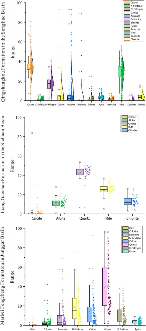
Figure 15. Box plots of mineral distribution of XRD data from cores of Gulong Shale oil Qingshankou Formation, Songliao Basin; Lianggao Mountain Formation, Sichuan Basin; and Mabei Fengcheng Formation, Junggar Basin.

Multiple migrations of the lake basin occurred during the depositional period of the Jurassic Liang Gaoshan Formation in the Sichuan Basin. Liang One section of the sedimentary period of the lake basin sedimentation centre from the southeast to the middle of Sichuan gradually expanding, belonging to the lake invasion period of the semi-deep lake - deep lake deposition, for a set of continuous 20–30 m thick dark grey, black shale, occasional thin layers of siltstone and mesocrustal layer. The centre of the lake basin during the sedimentary period of Liang Two section is located in Xichong and Guang’an areas in central Sichuan, and the top of Liang Two section is a set of 15–22 m thick organic matter-rich black shale interbedded with thin-layered powder-fine sandstone, with mesocrusts locally seen. The top of Liang Three section is a set of 5–15 m thick organic-rich black shale with thin layers of powder-fine sandstone (Figure 18C), with a thin shale thickness and a large distribution range. The multi-phase lake basin migration deposition process indicates that the lithology of the Liang Gaoshan Formation is relatively complex, and the shales in different layers, different areas, and different lithological combinations have different reservoir characteristics. Figure 18 shows that the main minerals in the Liang Gaoshan Formation in the Sichuan Basin are calcite, quartz, N-Feldspar, illite, chlorite, and a total of eight elements (Al, Fe, Mg, Si, Na, C, Ca, O).

Junggar Basin Mahu Depression Fengcheng Formation is located in the upper part of the Lower Permian, Fengcheng Formation depositional period, alkaline lake depositional environment, early volcanic activity, arid and hot climate, the development of a set of mud shale, dolomite, siltstone dominated by salinisation of the lake basin mixed deposition, from bottom to top is divided into the Feng One section (P1f1), the Feng Two (P1f2), the Feng Three (P1f3), the total thickness of 200∼1400 m. Feng One section is lake invasion deposition, with volcanic rocks and tuffs in the middle and lower part, and mudstone and dolomitic mudstone interbedded at the top; Feng Two section is high level deposition, forming a set of mudstone, dolomitic mudstone sandwiched with dolomitic siltstone and muddy dolomite, and interbedded with several sets of salt rocks; Feng Three section is lake recession deposition, with dolomitic mudstone in the middle and lower part, and siltstone, dolomitic siltstone, muddy siltstone, interbedded with colourful silty sandstone, and grey mudstone in the upper part. The upper part is dolomitic siltstone, muddy siltstone, interbedded colourful siltstone and grey mudstone. The main minerals of the Fengcheng Formation analysed by core experiments are chlorite, illite, dolomite, N-Feldspar, calcite, quartz, K-Feldspar, and pyrite, with a total of 10 elements (Si, Na, Al, Ca, Fe, S, Mg, K, C, O). Due to the different depositional conditions (lake level change, material supply, climate change, etc.), the sediment composition, and its combination form, etc., also changed in the three study areas. Mineral components based on the oxygen closure model of each mineral element dry weight ratio can be seen in Table 3, the well mineral profile processing results are shown in Figure 16.

Table 3

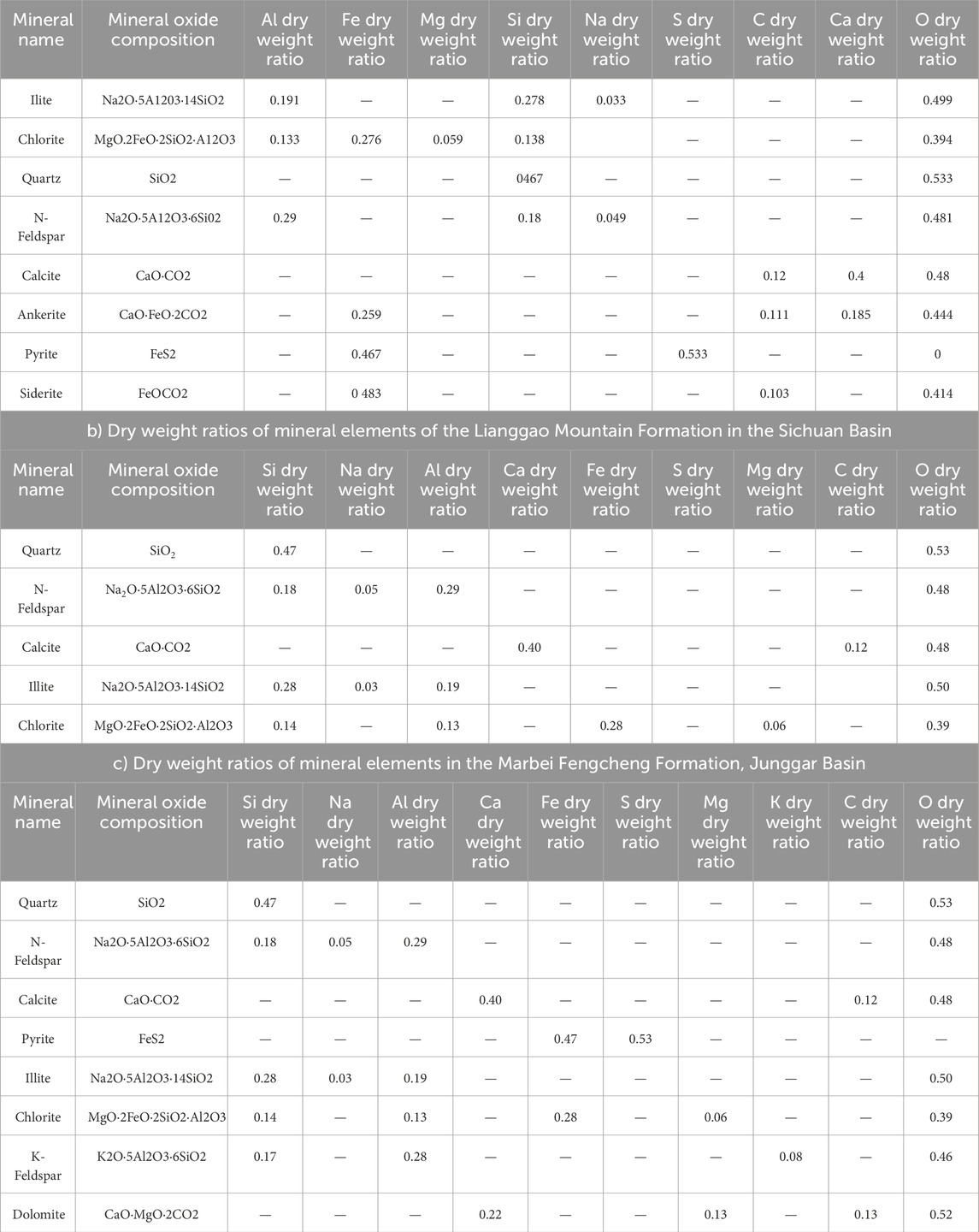
Table 3. a) Dry weight ratios of mineral elements in the Qingshankou Formation, Gulong Shale oil, Songliao Basin.

Figure 16

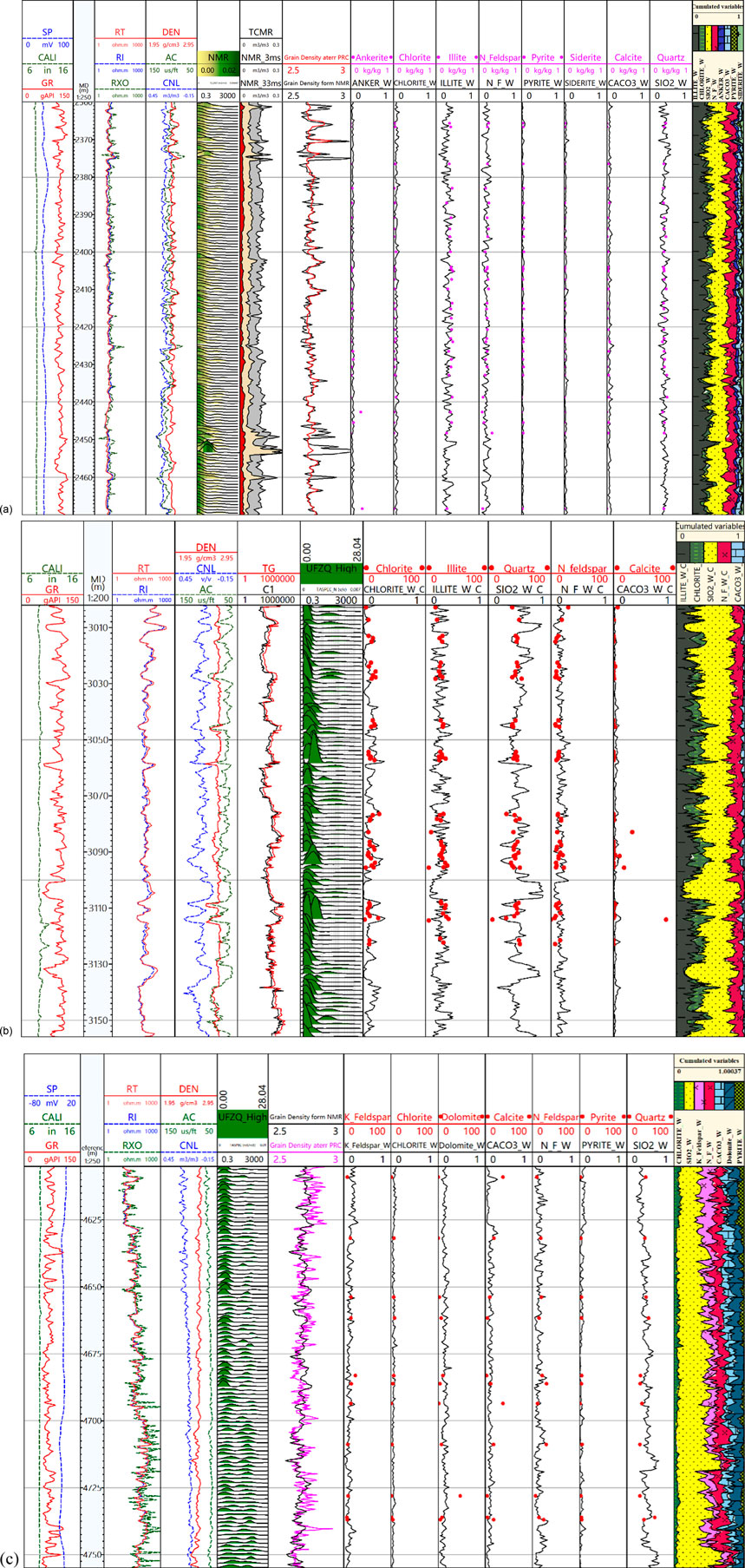
Figure 16. The interpretation results of lithology scanning logging for shale oil in the three major basins. (A) Mineral profile interpretation results after optimizing the objective function by fusing constraints in a well of mud-grained shale oil in Songliao Basin (B) Mineral profile interpretation results after optimizing the objective function by fusing constraints in a well of mud-textured shale oil in Sichuan Basin (C) Mineral profile interpretation results after optimizing the objective function with fusion constraints for a well of mélange shale oil in the Junggar Basin.

5.2 Analysis and application of processing results

Comparison of the mineral profile processing results of the three blocks with the core XRD experiments, the absolute error of all types of minerals is less than 5%, with good agreement, and the statistical table is shown in Table 4.

Table 4

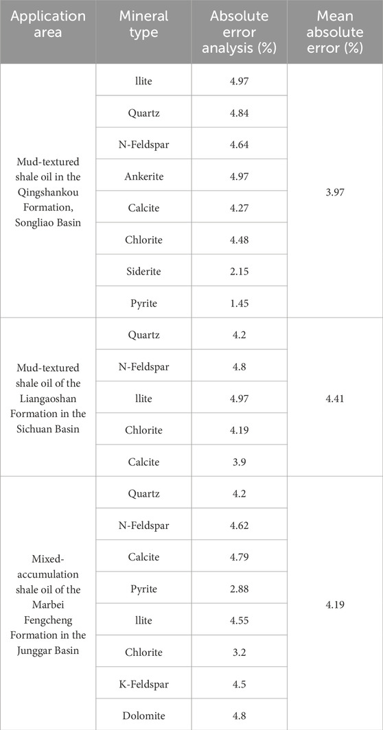
Table 4. Error analysis table of processing results.

LithoScanner logging processed continuous mineral profiles, based on the mineral distribution ternary map can be further completed lithology and lithofacies identification. Mineral distribution ternary map a commonly used combination of mineral dry weight to identify the lithology of the method, through the means of graphical display, analysis of different rock types or rock components of the proportionality between the relationship between the rock, and then divided into lithology, which can be intuitively reflected in the distribution of different lithological features and the law of change. Take Gulong Qingshankou Formation shale oil as an example, based on the geological characteristics of the Gulong area, three types of minerals, carbonate (iron dolomite + calcite), clay (illite + chlorite), and feldspar (feldspar + quartz), are selected as the three major classes in the ternary diagram shown in Figure 17, based on the mineral content, without considering the sedimentary structure and the total organic carbon (TOC) content of the Gulong shale oil Qingshankou Formation, which can be divided into Clay facies, long quartz facies, mixed facies, carbonate facies, four major categories.

Figure 17

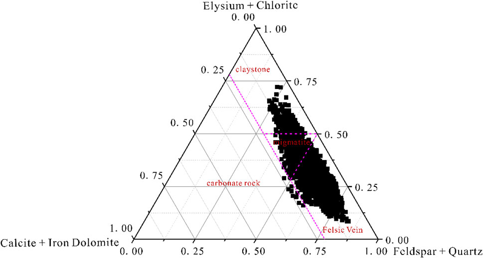
Figure 17. Classification of lithology based on mineral dry weight ternary diagram in Gulong area (The mineral ternary method for lithology classification is a commonly used method by geologists).

Petrography refers to rocks or rock assemblages formed in a certain sedimentary environment, while petrographic assemblage refers to the petrographic assemblage which is composed according to a certain superposition order, and can reflect the regular evolution of environmental conditions and the existence of a certain genesis connection. Traditional petrographic classification schemes for shales are generally based on the composition of inorganic minerals in the shale, the grain size of the clasts or grains, the sedimentary structure, and the total organic carbon (TOC) content. Gulong area grain layer development, its scale structure from microscopic to macroscopic there are different ways of superposition/mixing, different mineral components, rock types in different ways of rotary superposition, in the sedimentary body is manifested in the development of different lithology or facies of different types of grain layer structure, from the macroscopic structure can be classified into three major categories (grain layer, laminar, blocky), shale to the grain layer and the laminar structure of the predominant. At the same time, on the basis of the previous research, the macro-structural division criteria were established: textured (laminar density >=100 bars/m), laminated (10 bars/m=< laminar density <30 bars/m), massive (laminar density <10 bars/m), and the total organic carbon content (TOC) division criteria were rich in organic matter (>2%), medium in organic matter (1%–2%), and low in organic matter (0%–1%), and a total of 12 categories were classified. The final classification standard of petrography is shown in Table 5.

Table 5

Table 5. Division of petrographic phases in the Gurung area.

Summarising the petrographic assemblage patterns and characteristics of 23 wells in the Gulong area, which are classified into five types of assemblages, Class I: interbedded, laminated long quartz shale, Class II: interbedded long quartz, low to medium organic mixed shale, Class III: long quartz shale interbedded with mixed shale, Class IV: interbedded long quartz, mixed shale interbedded with carbonatite, Class V: interbedded long quartz, mixed shale interbedded with clayey shale. The results of this division are shown in Figure 18.

Figure 18

Figure 18. Petrographic assemblage types of the Qingshankou Formation in the Gulong area.

Statistical analysis of these five types of petrographic assemblage characteristics and commonly used shale oil three quality evaluation parameters, various types of petrographic assemblage characteristics in the shale oil three quality characteristics of each has its own advantages (Figure 19), Ⅰ type of petrographic assemblage is mainly composed of grainy long quartz shale, the main lithology of the brittle minerals content, the petrographic subphase is not obvious changes, the best compressibility, but its hydrocarbon generation ability is general, so the quality of the source rock and the quality of the reservoir is general. Class II petrographic assemblage is interbedded with mixed-quality textured shale and long quartz-quality textured shale, the overall structure of the main petrographic subphase is of interbedded type, the compressibility is average, poorer than that of Class I petrographic group, the S1 and oil-bearing porosity are slightly higher than that of Class I petrographic assemblage, and the quality of source rock and reservoir is good. Class III lithological assemblage is mainly long quartz shale interbedded with mixed shale, the overall structure of the main lithological subphase is interbedded, the compressibility is higher than that of Class II lithological assemblage as a whole, comparable to that of Class I lithological assemblage, and the quality of the source rock and the quality of the reservoir are the poorest. Class IV lithological assemblage is mainly long quartz, mixed shale interbedded with carbonate rock phases, the overall structure of the main lithological subphase is interbedded, the compressibility is comparable with Class II lithological assemblage, and the quality of the source rock and the quality of the reservoir is poorer than that of Class II lithological assemblage. Class IV lithological assemblages are mainly long quartz and mixed shale interbedded with clay shale phases, and the overall structure of the main lithological subphases is of interbedded type, with the clay shale phases as interbedded layers, so the compressibility is the poorest, but its hydrocarbon generation capacity is the best, and the quality of source rocks and reservoirs is the best.

Figure 19

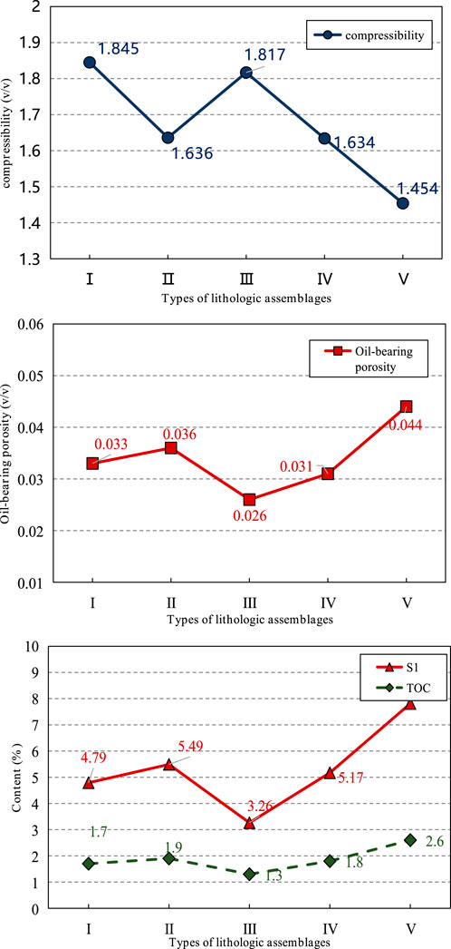
Figure 19. Distribution of three-quality evaluations of different lithologic combinations (In the Gulong area, the various lithofacies combinations show significant differentiation in the three qualities of shale oil, and can be well applied to explain the differences in shale oil production).

Collected five wells shot hole section and production data information, statistics on the thickness and percentage of the rock phase within the shot hole section, can be further analyzed rock phase and production capacity relationship. We can see in Figure 20, the lack of production from the E40 well is related to its single type of lithologic assemblage and the poor quality of the Class III lithologic reservoir and source rock; For wells A, B18, C6HC, and D16, which are rich in the variety of petrographic groups, the presence or absence of class V petrographic assemblage has a greater impact on their high or low production, and compared with wells B18, C6HC, and E40, the presence of class II and IV petrographic assemblage can enhance the reservoir output capacity.

Figure 20

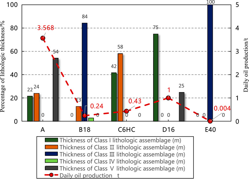
Figure 20. Table of single well production and thickness of lithologic assemblage in Gulong area.

6 Discussion

This paper primarily discusses the utilization of LithoScanner logging technology for processing shale oil formation data and lithology identification. By addressing issues in Schlumberger’s processing workflow, the main improvements and contributions focus on three aspects: 1, A core XRD experimental data normalization method is proposed. Specifically, density logging and nuclear magnetic resonance (NMR) logging data are integrated to calculate rock matrix density, which is then coupled with core XRD-derived dry weight density data for correction. 2, The introduction of a differential evolution (DE) algorithm enhances the original optimization method. This algorithm offers global optimization advantages, avoiding local optima. The improved approach better interprets lithological features under multi-logging data constraints, enhancing result reliability and geological significance. 3, A multi-data fusion workflow is developed. Elemental yield and core element dry weight data are preprocessed to improve stability, and multiple logging data (e.g., conventional density curves and NMR logging) are fused for processing and interpretation. This method strengthens data stability and accuracy, achieving an average error of less than 5% between calculated mineral dry weights and core XRD data.

The study provides a more precise and efficient geological evaluation tool for shale oil exploration. Additionally, key considerations for multi-type shale oil formations include:

Lithology interpretation workflows differ primarily in mineralogical diversity and vertical heterogeneity. Based on core XRD statistics, laminated shale oil exhibits fewer mineral types and weaker vertical heterogeneity compared to hybrid shale oil. Thus, during DE-based mineral profile inversion, appropriate parameters (e.g., smaller population sizes and mutation coefficients for laminated shale) must be selected to balance accuracy and reliability.

Certain minerals (e.g., borosilicate in hybrid shale) containing undetectable elements (e.g., boron, which cannot be measured by logging tools) cannot be interpreted via oxygen closure models due to the absence of boron data.

7 Conclusion

(1) During the processing of LithoScanner logging data, the oxygen closure model was reconstructed based on the XRD data of the returned core and the differential evolution algorithm was combined to invert the optimal solutions of various minerals. Different types of shale oil in Daqing Gulong, Sichuan Liangshan Mountain, Xinjiang Mabei have good application effect, and the average absolute error between the calculated dry weight of various minerals and the core XRD test dry weight can be less than 5%.

(2) For stratigraphic elements with a low dry weight percentage, the preprocessing of the data, along with the optimization of the objective function using a regularization term, is a major improvement for the interpretation accuracy enhancement.

(3) The improved processing interpretation scheme can be applied to many types of shale oil formations, with good application results, and the average absolute error between the calculated dry weights of various types of minerals and the dry weights of core xrd experiments can be less than 5%.

(4) Based on the continuous mineral profile obtained from LithoScanner logging, which can be used for the continuous division of petrography, lithofacies combinations significantly influence single-well productivity. Taking Daqing Gulong as an example, the combination of multiple types of petrography, and the percentage of the combination of V-type petrography, are the more important influencing factors on the production of its single well.

Data availability statement

The original contributions presented in the study are included in the article/supplementary material, further inquiries can be directed to the corresponding authors.

Author contributions

XH: Writing–original draft, Writing–review and editing. ZW: Writing–original draft. JS: Writing–review and editing. WY: Writing–review and editing. XC: Formal Analysis, Methodology, Writing–original draft. PL: Investigation, Writing–original draft. LZ: Investigation, Methodology, Writing–original draft.

Funding

The author(s) declare that no financial support was received for the research, authorship, and/or publication of this article.

Conflict of interest

Authors XH, ZW, JS, WY, XC, PL, and LZ were employed by Xinjiang Oilfield Company of PetroChina.

Generative AI statement

The author(s) declare that no Generative AI was used in the creation of this manuscript.

Publisher’s note

All claims expressed in this article are solely those of the authors and do not necessarily represent those of their affiliated organizations, or those of the publisher, the editors and the reviewers. Any product that may be evaluated in this article, or claim that may be made by its manufacturer, is not guaranteed or endorsed by the publisher.

References

Adeoti, L., Ikoro, C. O., Adesanya, O. Y., Ayuk, M., Oyeniran, T., and Allo, O. (2019). On the effectiveness of using quantitative AVO analysis in fluid and lithology discrimination in an offshore Niger Delta field,Nigeria. Ife J. Sci. 21 (1), 1–12. doi:10.4314/ijs.v21i1.1

CrossRef Full Text | Google Scholar

Cannon, D. E., and Coates, G. R. (1990). “Applying mineral knowledge to standard log interpretation,” in Transactions of the 31st annual SPWLA logging symposium, 24. Paper V).

Google Scholar

Craddock, P. R., Herron, S. L., and Badry, R. (2013). Hydrocarbon saturation from total organic carbon logs derived from inelastic and capture nuclear spectroscopy, in SPE Annual Technical Conference and Exhibition. SPE, D011S008R001.

Google Scholar

Gainitdinov, B., Meshalkin, Y., Chekhonin, E., Orlov, D., Zagranovskaya, J., Koroteev, D., et al. (2024). Predicting mineralogical composition in unconventional formations using machine learning and well logging data. International Petroleum Technology Conference. IPTC. IPTC-23487-EA.

CrossRef Full Text | Google Scholar

Galford, J., Truax, J., and Hrametz, A. (2009). “A new neutron-induced gamma-ray spectroscopy tool for geochemical logging,” in SPWLA annual logging symposium. SPWLA. SPWLA-2009-40058.

Google Scholar

Herron, M. M., Herron, S. L., Grau, J. A., and Seleznev, N. V. (2002). Real-time petrophysical analysis in siliciclastics from the integration of spectroscopy and triple-combo logging. SPE Annu. Tech. Conf. Exhib SPE: SPE-77631-MS.

Google Scholar

Herron, S., Herron, M., Pirie, I., Saldungaray, P., Craddock, P. R., Charsky, A. M., et al. (2014). Application and quality control of core data for the development and validation of elemental spectroscopy log interpretation. Petrophysics 55 (05), 392–414.

Google Scholar

Herron, S. L., and Herron, M. M. (2000). Application of nuclear spectroscopy logs to the derivation of formation matrix density, Transactions of the SPWLA 41st Annual Logging Symposium, 4-7 June. Dallas, Texas, USA. Paper JJ.

Google Scholar

Juntao, L., Shu, C., Liu, F., Zhang, B. M., Yuan, C., and Su, B. (2018). A method for improving the evaluation of elemental concentrations measured by geochemical well logging. J. Radioanalytical Nucl. Chem. 317 (2), 1113–1121. doi:10.1007/s10967-018-5986-y

CrossRef Full Text | Google Scholar

Lai, F. Q., Liu, Y. j., Tan, X. F., Wang, R., Peng, S., and Gao, X. (2024). A composite water saturation model of continental mixed shale oil reservoirs based on complex lithology identification!. Geol. J. 59 (4), 1401–1415. doi:10.1002/gj.4934

CrossRef Full Text | Google Scholar

Lai, J., Wang, G., Fan, Q., Pang, X., Li, H., Zhao, F., et al. (2022). Geophysical well-log evaluation in the era of unconventional hydrocarbon resources: a review on current status and prospects. Surv. Geophys. 43 (3), 913–957. doi:10.1007/s10712-022-09705-4

CrossRef Full Text | Google Scholar

Liao, D. L. (2015). Interpretation and application of ECS logging data in shale formations. Pet. Drill. Tech. 43 (4), 102–107.

Google Scholar

Mao, R., Shen, Z. M., Zhang, H., Chen, S., and Fan, H. (2022). Lithology identification for diamictite based on lithology scan logging: a case study on Fengcheng Formation, Mahu sag. Xinjiang Pet. Geol. 43 (06), 743–749.

Google Scholar

Miles, J., and Badry, R. (2014). Borehole carbon corrections enable accurate TOC determination from nuclear spectroscopy. Petrophysics 55 (03), 219–228.

Google Scholar

Mosse, L., Rodriguez, L. M., Chiapello, E., Lambert, L., Leduc, J.P., Decoster, E., et al. (2014). “Accurate lithology and TOC obtained from an induced gamma ray spectroscopy tool,” in Two major challenges in shale reservoirs Simposio Evaluación de Formaciones. IX Congreso Argentino de Exploración y Desarrollo de Hidrocarburos IAPG. Mendoza, Argentina.

Google Scholar

Radtke, R. J., Lorente, M., and Stoller, C. (2012). A new capture and in elastic spectroscopy tool takes geochemical logging to the next level SPWLA 53rd Annual Logging Symposium. Paper AAA.

Google Scholar

Sun, J. M., Jiang, D., and Yin, L. (2014). A method for determining mineral content by formation element logging. Nat. Gas. Ind. 34 (02), 42–47.

Google Scholar

van den ord, R. J. (1991). Evaluation of geochemical logging. Log Analyst. Junuary-February.

Google Scholar

Waters, C. N., Vane, C. H., Kemp, S. J., Haslam, R. B., Hough, E., and Moss-Hayes, V. L. (2020). Lithological and chemostratigraphic discrimination of facies within the Bowland shale formation within the Craven and Edile basins, United Kingdom. Pet. Geosci. 26 (2), 325–345. doi:10.1144/petgeo2018-039

CrossRef Full Text | Google Scholar

Yang, X. Q., and Wang, H. (2012). Litho scanner. Well Logging Technol. 36 (06), 568.

Google Scholar

Zhang, H., and Li, Y. (2022). Research on identification model of element logging shale formation based on IPSO-SVM. Petroleum 8 (2), 185–191. doi:10.1016/j.petlm.2021.04.004

CrossRef Full Text | Google Scholar

Zhang, Z., Song, Y., Yan, W., Yin, S., Zheng, J., and Li, C. (2024). Integrated geological quality evaluation using advanced wireline logs and core data: a case study on high clay shale oil reservoir in China. J. Geophys. Eng., gxae093.

Google Scholar

Zhao, H. B., Zheng, J. D., Zhang, Z. Q., Qin, H., Wang, C., Zhu, J., et al. (2024). Research progress and prospects of oil saturation evaluation methods in shale oil reservoirs. Processes 59 (5), 2421. doi:10.3390/pr12112421

CrossRef Full Text | Google Scholar