Comparison between plant fossil assemblages and simulated biomes across the Permian-Triassic Boundary

Terrestrial ecosystems underwent extreme shifts in composition, following extensive degassing associated with the Siberian Traps near the Permian–Triassic boundary (PTB). These climatic perturbations are recorded in land plant macrofossil assemblages, which reflect complex changes in major biomes at the stage level. In this study, we quantitatively compare the major biomes reconstructed from the plant macrofossil assemblage data with those derived from coupled climate–vegetation simulations across the PTB. We focus on five stages across the PTB, from the Wuchiapingian to the Anisian. Our findings indicate that a shift from a cold climatic state to one with a mean surface temperature approximately $10°$C higher is consistent with observed changes over time in plant biomes, as documented in macrofossil records. In contrast, vegetation patterns during the Induan stage suggest strong variability, precluding a univocal attribution to a stable climate.

1 Introduction

The Permian–Triassic boundary (PTB) mass extinction occurred ca. 252 million years ago and was marked by the most severe biotic crisis in the Phanerozoic (Raup and Sepkoski, 1982; Stanley, 2016). Extreme reductions in both marine and terrestrial animals were recorded, most likely caused by extensive degassing associated with the Siberian Traps (Renne and Basu, 1991; Renne et al., 1995; Sibik et al., 2015; Burgess et al., 2017; Svensen et al., 2018; Davydov, 2021; Callegaro et al., 2021). In the PTB aftermath, life on Earth had to drastically adjust to repeated changes in climate and the carbon cycle for several million years. This crisis in the faunal realm was coeval to complex shifts in composition in terrestrial ecosystems that were not limited to a single event (Looy et al., 2001; Hochuli et al., 2016; Schneebeli-Hermann, 2020). Recent studies show that land plant macro- and microfossil (spores and pollen) records of the Early Triassic do not provide strong evidence for a sudden and catastrophic biodiversity loss coeval with the faunal diversity loss at the PTB (Nowak et al., 2019). Nonetheless, major changes in regional and global environmental conditions and flora composition occurred throughout the Early Triassic (Hochuli et al., 2016; Fielding et al., 2019; Schneebeli-Hermann, 2020; Mays et al., 2021; Mays and McLoughlin, 2022). This includes the abrupt extirpation of the primary coal-forming carbon sinks, such as the Glossopteris biome of Gondwana (Mays et al., 2019; Vajda et al., 2020; Mays et al., 2021) and the tropical gigantopterid forests of East Asia at the end of the Permian (Chu et al., 2020). Shifts between a lycophyte-dominated (spore-producing vascular plants) and a gymnosperm-dominated (seed-producing plants, including conifers) vegetation coincided, respectively, with a succession of warm and cold climatic conditions (Galfetti et al., 2007b; Schneebeli-Hermann, 2020). Changes from gymnosperm- to lycophyte-dominated vegetation, as recorded in palynomorph assemblages from subtropical locations, occurred at the PTB and during the earliest Triassic Induan stage (at the Griesbachian–Dienerian substage boundary), whereas the shift from lycophyte- to gymnosperm-dominated vegetation occurred in the subsequent Olenekian stage (at the middle-late Smithian boundary), with transient regimes observed before and after this transition. Spores and pollen from higher latitudes record similar changes in relative abundance during the Early Triassic (Hochuli et al., 2010; Hochuli et al., 2016).

The macrofossil assemblages described by Nowak et al. (2019) were later used to reconstruct major biomes (Nowak et al., 2020), defined as areas with comparable, climatically controlled plant and animal assemblages (Ziegler, 1990; Walter, 2012). A reduction in biome diversity from the Permian to the Early Triassic was observed and was associated with a climate shift characterized by an increase in seasonality. This period of high variability was followed by a stable phase that lasted through the Middle Triassic, with comparable biomes from the Olenekian to the Ladinian. Microfossils were excluded from the reconstruction of the biome distribution as their source areas can be vast (regional) and not representative of the depositional site (Nowak et al., 2020).

The analysis provided by Nowak et al. (2020) was performed with a temporal resolution at the stage level from the Wuchiapingian to the Ladinian. In the present paper, we will expand upon this analysis using climate simulations obtained by the offline coupling between a general circulation model (MITgcm) and a vegetation model (BIOME4). The climate simulations were performed using the paleogeographic configuration provided by PANALESIS (Vérard, 2019; Vérard, 2021) for the PTB, as described by Ragon et al. (2024). Interestingly, three alternative climatic steady states (denoted as cold, warm, and hot attractors) have been found for the same boundary conditions, with mean surface air temperatures (SATs) ranging from $17°$C to $37°$C, as shown in the bifurcation diagram in Figure 1 in terms of the atmospheric ${\text{CO}}_2$ content. This diagram describes the dynamical backbone structure of the climate system (Ghil and Lucarini, 2020; Margazoglou et al., 2021; Brunetti and Ragon, 2023), showing the stable branches of the steady states, their extent, the position of tipping points, and possible hysteresis paths and tipping mechanisms to shift from one attractor to another (Ashwin et al., 2012).

Figure 1

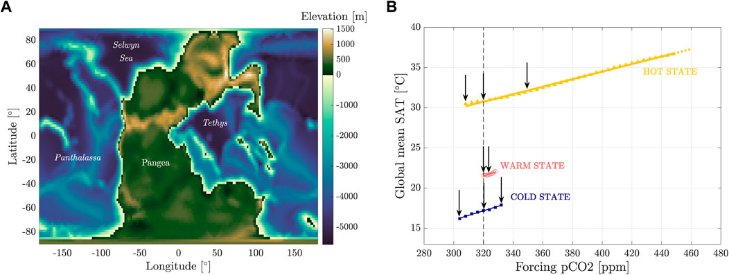
Figure 1. Permian–Triassic paleogeography (A) and corresponding bifurcation diagram (B) in terms of the equilibrium values of the global mean surface air temperature vs. the atmospheric ${\text{CO}}_2$ content (Ragon et al., 2024). Yellow triangles, red circles, and blue squares represent averages over 100 years for a given forcing value for the hot, warm, and cold attractors, respectively. Black arrows identify the location of coupling simulations between MITgcm and the vegetation model BIOME 4. The vertical dashed line corresponds to 320 ppm, the forcing value at which coupling is performed in the three attractors.

The presence of alternative attractors and the structure of the bifurcation diagram in Figure 1 suggest a potential explanation for shifts in composition observed in terrestrial ecosystems across the PTB as shifts between attractors. These transitions may have induced strong climatic variations in both atmospheric and oceanic circulations, impacting the whole climate system (Ragon et al., 2024; Rogger et al., 2024). Perturbations of the carbon cycle, as a consequence of the outgassing associated with the Siberian Traps, may have triggered not only bifurcation-induced tipping between the cold and hot states, with repeated activation of the hysteresis loop between these two states, but also noise- or rate-induced tipping between the three attractors (Ashwin et al., 2012; Brunetti and Ragon, 2023; Feudel, 2023).

The aim of this paper is to assess whether the changes in global vegetation patterns, as recorded in land–plant macrofossil assemblages at the stage level and presented by Nowak et al. (2020), can be explained by tipping between the simulated climatic attractors. We will quantitatively compare the modeled major vegetational biomes for the hot, warm, and cold states with the land–plant macrofossil assemblages compiled by Nowak et al. (2019) and Nowak et al. (2020), spanning from the Lopingian (starting at 259.51 Ma and including the Wuchiapingian and the Changhsingian) to the early Middle Triassic ($\sim$242 Ma). This corresponds to five stages, namely, Wuchiapingian starting at 259.51 Ma, Changhsingian at 254.14 Ma, Induan at 251.902 Ma, Olenekian at 251.2 Ma, and Anisian at 247.2 Ma (Cohen et al., 2013).

2 Methods

2.1 Paleogeographic reconstruction

The Permian–Triassic paleogeography is derived from PANALESIS (Vérard, 2019; Vérard, 2021), a global plate tectonic model providing maps every 10 Myr from 888 Ma (Tonian) to the present. The PANALESIS paleogeography for the PTB, which we use as a fixed boundary condition in our climate simulations, has proven to be in good agreement with geochemical and paleontological records (Chablais et al., 2011; Peyrotty et al., 2020; Bucur et al., 2020; Le Houedec et al., 2024), particularly in locating elements within the intertropical zone. The location of island arcs, continental ribbons, and even parts of Pangea, such as South China, remains, however, subject to uncertainties, with latitudes potentially varying up to ca. $10°$. The raw PANALESIS map was adapted to the climate model horizontal resolution of $2.8°$ ($\sim 300$ km). Specifically, seaways narrower than a few pixels were enlarged, while the smallest ones, along with epicontinental seas and lakes, were closed. The resulting topography used in the simulations is shown in Figure 1A.

2.2 Plant fossil records

The study by Nowak et al. (2020) was based on a dataset of plant macrofossil assemblages from Nowak et al. (2019), which is a compilation of previously published and unpublished plant fossil collections. This dataset is used in the present paper to determine major biomes at the stage level, spanning from the Wuchiapingian to the Anisian. Each plant genus is associated with the major biome(s) it could potentially occur in, possibly exclusively (i.e., when a plant genus is known to be limited to habitats aligned with a certain biome; see Supplementary Table S2 in Nowak et al. (2020) for details).

The records are aggregated within a moving 100-km radius, where each genus is assigned a weight corresponding to the inverse of the number of major biome(s) it is associated with. For each aggregated assemblage, a vote for all possible biomes is then tallied based on the weights of all present genera. The final major biome is determined based on either i) the exclusive major biome if a characteristic representative is present, ii) the major biome whose combined weight is $>50\%$ in the area, or iii) the major biome manually assigned by the authors considering taxa, location, and neighborhood (if the combined weight for each calculated biome is $<50\%$). The resulting major biome distribution, thus, reflects the distribution of all plant macrofossil collections and corresponds to the area with comparable, climatically controlled plant and animal assemblages (Nowak et al., 2020). This method helps reduce the uncertainty in location and short-scale variability. However, some of the manual biome assignments are tenuous and mainly based on surrounding data points. In these cases, if a single calculated biome is indicated as the most likely one (as opposed to multiple candidates with similar combined weights, each being the case in approximately half of the manual assignments or a quarter of all aggregated assemblages), we use the latter in the present study. This approach aims to keep data points independent without introducing new interpretations.

The classification of major biomes used in this study comprises six categories, which are mostly adapted from those in Nowak et al. (2020), which, in turn, followed the set of biomes introduced by Ziegler (1990) as far as they could be applied to the fossil dataset at hand. The resulting simplified major biomes are briefly described as follows: the tropical everwet major biome includes various vegetation types developing under constantly hot and humid conditions, typically near the equator, but it can extend up to mid-latitudes. The tropical summerwet major biome represents intermediate vegetation between tropical everwet and desert, found in middle to low latitudes with marked seasonality and wet summers. The desert major biome includes both subtropical and mid-latitude deserts but is generalized to all latitudes in this study and is marked by water deficiency. The warm-to-cool temperate major biome encompasses vegetation ranging from evergreen (i.e., plants that keep their needles or leaves all year) to deciduous (i.e., plants that shed their leaves in autumn), affected by seasonal changes in climatic conditions. The cold temperate major biome is associated with areas with low evaporation, where the short growing season is mainly controlled by temperature and sunshine. The tundra major biome has a very short growing season and was not recorded by Nowak et al. (2020).

2.3 Vegetation distribution along the stable branches

The simulated vegetation distribution is different between the three attractors but also varies along each stable branch, together with the atmospheric ${\text{CO}}_2$ content. The range of vegetation pattern on each attractor is determined by applying the asynchronous coupling procedure between the MITgcm and BIOME 4 models, as described in Supplementary Appendix SA at various positions along the branches. This includes a common value of 320 ppm and, in general, at the edges of each branch (see Figure 1B). For the warm state, which has a narrow stable branch, only two positions are selected, at 320 ppm and near the upper edge of the branch (328 ppm). The two models, the climate model MITgcm (Marshall et al., 1997a; Marshall et al., 1997b; Adcroft et al., 2004; Marshall et al., 2004) and the vegetation model BIOME 4 (Haxeltine and Prentice, 1996; Kaplan, 2001; Kaplan et al., 2003), have been described in the Methods section of Ragon et al. (2024). The convergence criteria between MITgcm and BIOME 4 are 1) the global SAT does not change between two iterations (within the uncertainty) and 2) the land surface fraction where albedo varies between two iterations is smaller than 10%. The corresponding values and surface imbalance over the ocean at each iteration of the coupling procedure are reported in Supplementary Table S6.

The biomes resulting from the simulations (28 biomes; see Kaplan, 2001) are grouped in the same major biomes described in Section 2.2 to facilitate the comparison with the geological records provided by Nowak et al. (2020) and eliminate perturbations coming from small differences between similar biomes. The corresponding classification is described in Table 1.

Table 1

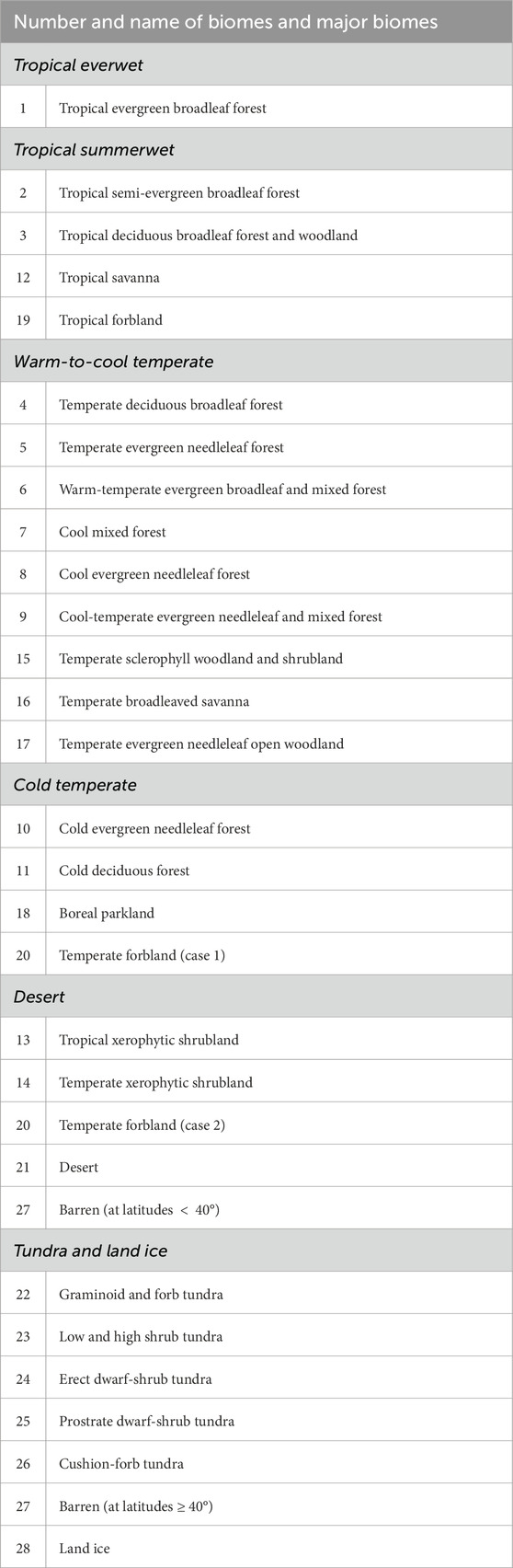
Table 1. Correspondence between the 28 biomes represented in the BIOME 4 model and the major biomes adapted from Nowak et al. (2020) (in italics). Cases 1 and 2 refer to alternative classifications of the temperate forbland biome.

The present-day “grassland” is replaced by the herbaceous non-graminoid “forbland” because graminoids only appeared during the Cretaceous–Cenozoic (Gradstein and Kerp, 2012). There is consequently no direct equivalence between simulated grasslands and any fossil assemblage or fossil-based biome from the Permian and Triassic, but we can infer likely correspondences based on the climatic conditions they represent. Both tropical savanna and tropical forbland biomes have been included in the tropical summerwet major biome. Even if they slightly differ from the broadleaf forest category, their seasonality has been considered the main argument for their classification. The classification of barren, a desertic biome mainly associated with polar regions in present-day vegetation, is distinguished by the latitude of formation: the desert major biome is found below 40$°$ latitude, while tundra is located above.

The criteria for temperate forbland biome in BIOME 4 correspond to desert-like conditions, more than everwet or seasonally wet. However, our simulations show that this biome is mostly formed in high latitudes, $\gtrsim 40°$ (see for example gray areas in Figure 2). In polar regions, reduced evaporation gives rise to cold temperate vegetation, allowing it to thrive instead of forming deserts. For that reason, temperate forbland is classified as a cold temperate major biome (case 1 in Table 1). For completeness, we repeat the same analysis with an alternative interpretation, whereby temperate forbland is classified as a desert (case 2 in Table 1) in Section 3.4.

Figure 2

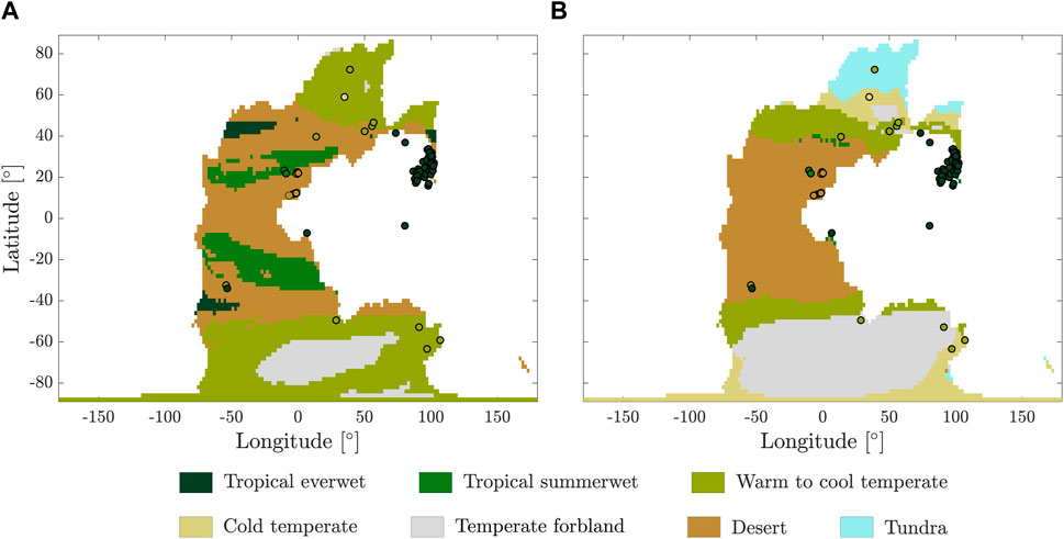
Figure 2. Comparison of plant fossil assemblages of Wuchiapingian age (259.51–254.14 Ma) superposed with major biomes modeled at 320 ppm for the (A) hot state and (B) cold state.

2.4 Similarity between geological records and modeled biomes

The paleontological record provides local information on vegetation, while the model simulates broader areas, posing a challenge for the direct comparison between the two. Visual comparisons (see example in Figure 2) can offer valuable insights into how well the simulation aligns with the records; however, this approach is not quantitative and does not always provide a clear answer.

Each plant fossil assemblage record is assigned to the model-grid cell corresponding to its location. Although the single outcrops are considered independent, their spatial resolution is sometimes higher than that of the model [i.e., records fall within the same grid cell of $\sim$(300 km)²]. Because typical statistical fluctuations decrease with the square root of the number of observations, each distance is weighted based on the number of similar individual records in the same cell (see Equation 2). This results in the merging of plant fossil assemblages, representing the same biome within the same cell, thereby increasing their confidence. The merging contributes to a reduction in sample sizes $n$: from 97 to 56 (Wuchiapingian), 59 to 43 (Changhsingian), 66 to 46 (Induan), 88 to 42 (Olenekian), and 202 to 64 (Anisian). Note that the weight is applied only for the mean distance calculation, whereas for the median, only one record is considered among the identical ones within the same grid cell (see Section 2.5).

The similarity between the plant macrofossil record at a given stage and the simulated vegetation distribution of an attractor is estimated as follows. For each reported assemblage of fossil plants, we compute the smallest geodesic distance $d$ to the nearest region where the same major biome has been predicted by the simulation, given by

$d=R\cdot \left[\arccos \left(\sin \left({\varphi }_M\right)\sin \left({\varphi }_F\right)+\cos \left({\varphi }_M\right)\cos \left({\varphi }_F\right)\cos \left({\lambda }_F-{\lambda }_M\right)\right)\right],(1)$

where $R=6371$ km is the Earth radius, $\varphi$ is the latitude, $\lambda$ is the longitude, and indices refer to the position of the fossil record $(F)$ and the nearest point on the map where the considered major biome is simulated $(M)$. Figure 3 shows an example with a simulation and few paleobotanical records, where arrows correspond to the distance between the record and the nearest cell with the same major biome. We have checked that if the model predicts the same major biome at the position where it has been observed, then the distance is 0 (see the two records without arrow in Figure 3). When a major biome present in the fossil record does not appear in a simulation, the distance is arbitrarily set to the longest possible distance, i.e., the distance between the two poles, $\pi \cdot R\sim 2\cdot 10^7$ m.

Figure 3

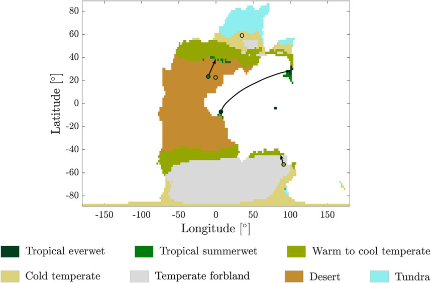
Figure 3. Example of the calculation of the smallest geodesic distance between geological records (circles with black contours) and the nearest region where the same major biome has been predicted by the simulation.

We define the weighted mean distance $\bar{d}$ of the ensemble as follows:

$\bar{d}=\frac{{\sum }_{i=1}^n\frac{1}{\sqrt{n_i}}{d}_i}{{\sum }_{i=1}^n\frac{1}{\sqrt{n_i}}},(2)$

where $d_i$ is given by Equation 1 for each observation i, n is the sample size, $n_i$ is the number of co-located identical records, and $\frac{1}{\sqrt{n_i}}$ is the weight applied to each point. The associated variance V is as follows:

$V=\frac{{\sum }_{i=1}^n\frac{1}{\sqrt{n_i}}{\left(d_i-\bar{d}\right)}^2}{{\sum }_{i=1}^n\frac{1}{\sqrt{n_i}}},(3)$

2.5 Statistical tests

The distances $d_i$ are calculated for each combination of fossil records (for each stage) and simulation (for each attractor and ${\text{CO}}_2$ value), together forming a sample. For a given stage, eight samples corresponding to the eight simulations are available. The one minimizing the mean distance $\bar{d}$ (or median distance) is assumed to better represent the vegetation distribution recorded at that stage. The difference between this sample and the others can either be due to i) a real difference between the populations from which the samples are drawn or ii) sampling fluctuations, meaning that geological records do not permit discrimination between the two simulations. In the first case, the simulation minimizing $\bar{d}$ is significantly better at reproducing the recorded vegetation, while in the second case, the data do not allow for the clear determination of which attractor minimizes the distance. To distinguish between these two cases, statistical tests are employed. These tests determine whether the difference between two samples, $A$ and $B$, is significant.

The utilization of several methods (on means and medians), together with the classification of the temperate forbland biome into two different major biomes (cases 1 and 2 in Table 1), allows us to test the robustness of the results (see also Supplementary Appendix SB).

2.5.1 Testing difference between means: $t$-test

We assume that the distributions of $d_i$ follow a normal distribution with mean $\bar{d}$ and variance $V$ (given, respectively, in Equations 2, 3) and that our sample is sufficiently large to approximate the variance ${\sigma }^2$ of the population distribution by the variance of the sample distribution $V$. The deviation from the null hypothesis (i.e., two combinations of a set of fossil records with a simulation, $A$ and $B$, have the same mean: ${\bar{d}}_A={\bar{d}}_B$) can be tested using (Bouyer, 1996)

$Z_0=\frac{\left({\bar{d}}_A-{\bar{d}}_B\right)}{\sqrt{\frac{V_A}{n_A}+\frac{V_B}{n_B}}},(4)$

where $n_A$ and $n_B$ are the sample sizes. This quantity can be converted into the probability $p$ of obtaining a difference equal to or larger than the observed one, according to the null hypothesis. The $p$-value is given by

$p=0.5\left(1-\text{erf}\left(\frac{Z_0}{\sqrt{2}}\right)\right),(5)$

where Z₀ is given in Equation 4 and $\text{erf}$ is the error function. The null hypothesis is rejected when $p<5\%$ for the unilateral test. In this study, sample $A$ always refers to the one minimizing $\bar{d}$, while sample $B$ is one of the other samples such that ${\bar{d}}_B>{\bar{d}}_A$. The estimated probability answers the following question: is ${\bar{d}}_B$ significantly larger than ${\bar{d}}_A$? the probability is 50% only if ${\bar{d}}_A={\bar{d}}_B$.

2.5.2 Testing difference between medians: Mood-test

The $t$-test on means is based on the hypothesis that the populations follow a normal distribution. An alternative is the Mood-test for medians, a method without any assumption about the shape of the distribution, the only requirement being that the two populations have the same shape (Mood, 1950; Zar, 2010). Moreover, the median is less sensitive to outlier values than the mean and thus to the missing biomes in the simulations, for which we arbitrarily set the maximal distance ($\sim 2\cdot 10^7$ m).

The Mood-test is applied to determine whether the difference in the median value of the distances $d_i$ for two attractors is significant, the null hypothesis being $m_A=m_B$. This test consists of 1) the determination of the ‘grand median’ of the two reunited samples, 2) the construction of the contingency table to count the number of distances $d_i$ above and below the grand median in each sample, and 3) testing the independence of the two categories through a ${\chi }^2$ test. The test is performed using median_test from the scipy-stats Python library.

A 5% threshold is used, as for the $t$-test, to reject the null hypothesis. However, for two identical samples, the probability is $p=100\%$ since the Mood-test is bilateral.

3 Results

3.1 Simulation maps

The simulated distribution of the major biomes corresponding to the attractors at various atmospheric ${\text{CO}}_2$ contents is shown in Figure 4. Tundra, barren, and land ice biomes, which have no correspondence in the macrofossil assemblages, are mostly present in polar regions in the cold and warm states, especially at the northern polar latitudes coinciding with the sea ice extent (Ragon et al., 2024).

Figure 4

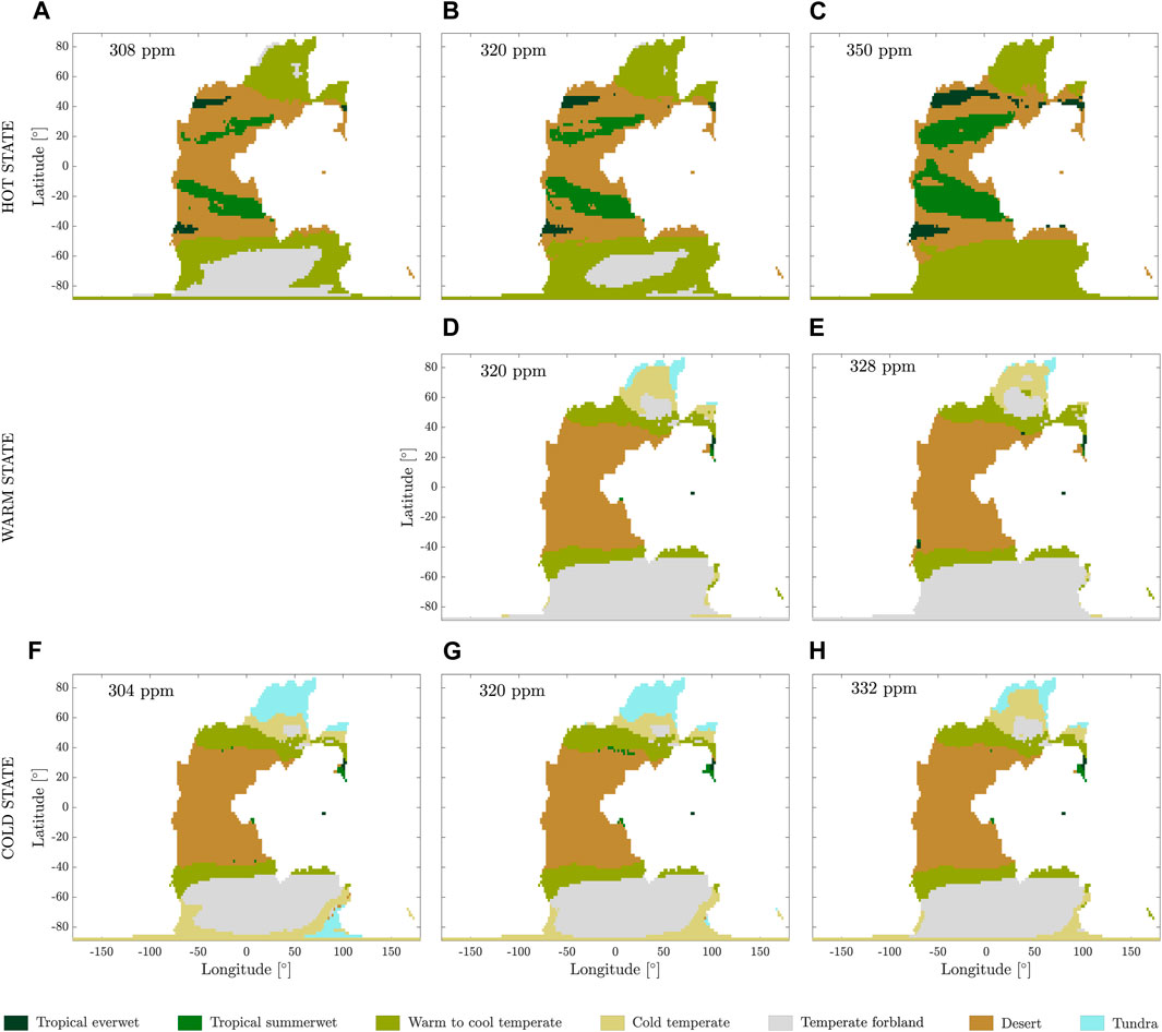
Figure 4. Distribution of the major biomes (see Table 1) for (A–C) hot, (D, E) warm, and (F–H) cold states, with the atmospheric ${\text{CO}}_2$ content varying, as indicated next to the labels. The white area corresponds to ocean.

The simulated major biomes in the cold and warm states (Figures 4D–H) are both dominated by desert at tropical and subtropical latitudes. Along 60$°$ latitude, a band of warm-to-cool temperate vegetation is present, whereas in polar regions, cold temperate plants are favored and switch into tundra when moving poleward. The space occupied by the tundra in the northern polar region reduces in favor of cold temperate as the atmospheric ${\text{CO}}_2$ content increases along the stable branch. The changes in atmospheric ${\text{CO}}_2$ content mainly affect the biomes in the high latitudes of the northern hemisphere in both attractors. In the southern polar region, the vegetation is largely dominated by temperate forbland (i.e., either cold temperate or desert major biomes, as discussed in Section 2.3).

In the hot state, the warm-to-cool temperate major biome is also present but shifted poleward compared to the other attractors, so it dominates in the northern polar region. The southern polar region is occupied by both the warm-to-cool temperate major biome and temperate forbland, with the extent of the latter reducing as the atmospheric ${\text{CO}}_2$ content increases (see Figures 4A–C). At tropical and subtropical latitudes, desert areas are generally present, and plants adapted to tropical summerwet and everwet environments are well-distributed along the tropics and 50$°$ latitude, respectively. Their extent increases together with the atmospheric ${\text{CO}}_2$ content along the hot-state branch. In general, the increase in atmospheric ${\text{CO}}_2$ content favors warmer and wetter major biomes: tropical everwet/summerwet over desert in mid-latitudes/tropical regions and warm-to-cool temperate over temperate forbland in the southern polar region.

3.2 Test on the mean values

Figure 5 shows, at the five considered stages, the mean distance $\bar{d}$ and associated standard error $\sqrt{V}$ (green circles and bars, respectively) for each simulation, along with the $p$-value. See also Supplementary Table S1.

Figure 5

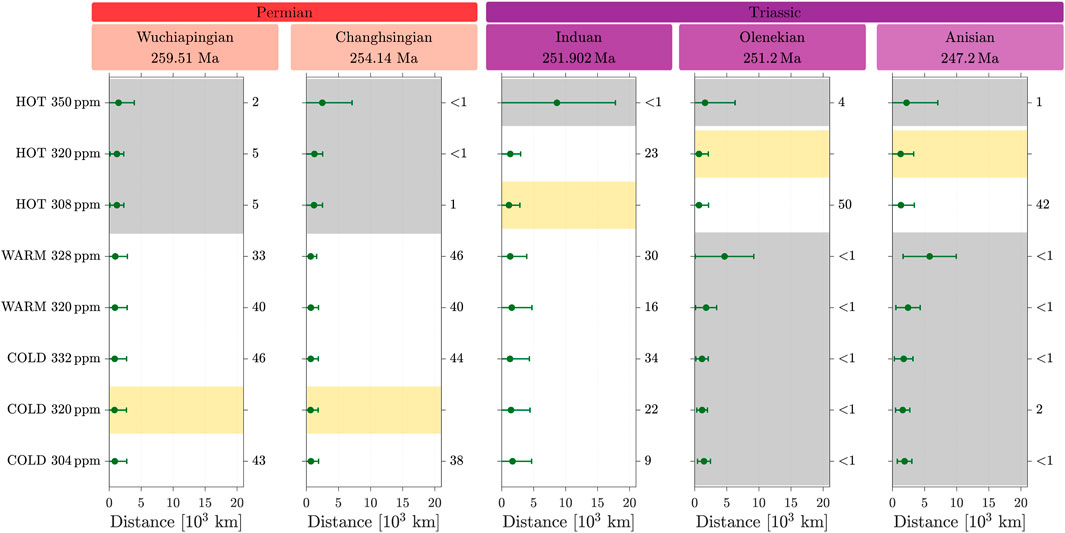
Figure 5. Weighted-mean and standard deviation of the distances computed between each of the eight simulations and geological records for the five stages. For each stage, the yellow area indicates the simulation minimizing the mean distance. The numbers on the right correspond to the $p$-values [%] of the difference between each distribution and the one highlighted in yellow (Equation 5), rounded to a percent. When rounding with 0 digits leads to 0%, the notation $<1\%$ is used instead. Gray areas indicate statistically significant differences. In this figure, temperate forbland is included in the cold temperate major biome (case 1).

For the two oldest stages, the Wuchiapingian and the Changhsingian (Lopingian), the vegetation distribution modeled for the cold state at 320 ppm provides the best match with the fossil records. However, it is not significantly different from the vegetation distribution modeled at other positions on the cold branch or from the warm state. In contrast, the vegetation simulated in the hot state is significantly different, and thus, it is not a good candidate to reproduce the records of these stages.

In the case of the Induan, the hot state at 308 ppm minimizes $\bar{d}$ but is not statistically different from any of the other simulated conditions, except for the upper branch of the hot state, which can be excluded. For both the Olenekian and Anisian, the lower part of the hot-state branch, i.e., at 308 ppm and 320 ppm, significantly differs from all the other conditions and better matches the records.

These results suggest a transition from the cold or warm state in the Lopingian to the hot state in the Olenekian, in concordance with the global warming recorded from the Lopingian to the Early Triassic (Retallack, 1999; Joachimski et al., 2012). The hot state persists during the Anisian, thus marking the stabilization of the climate system, as recorded, for example, in ${\delta }^{13}$C isotopic records (Payne et al., 2004). The unclear signal during the Induan might be the result of oscillations occurring at smaller temporal scales, as observed in the proxy of temperature ${\delta }^{18}$O (Romano et al., 2013).

3.3 Test on the median values

The test on medians shows a trend comparable to what is observed for that on means, as shown in Figure 6; Supplementary Table S2. For both the Wuchiapingian and the Changhsingian, the cold state, not statistically different along the branch or from the warm state, has a smaller median and thus matches better with the data, while the hot state has a significantly larger median and thus can be excluded.

Figure 6

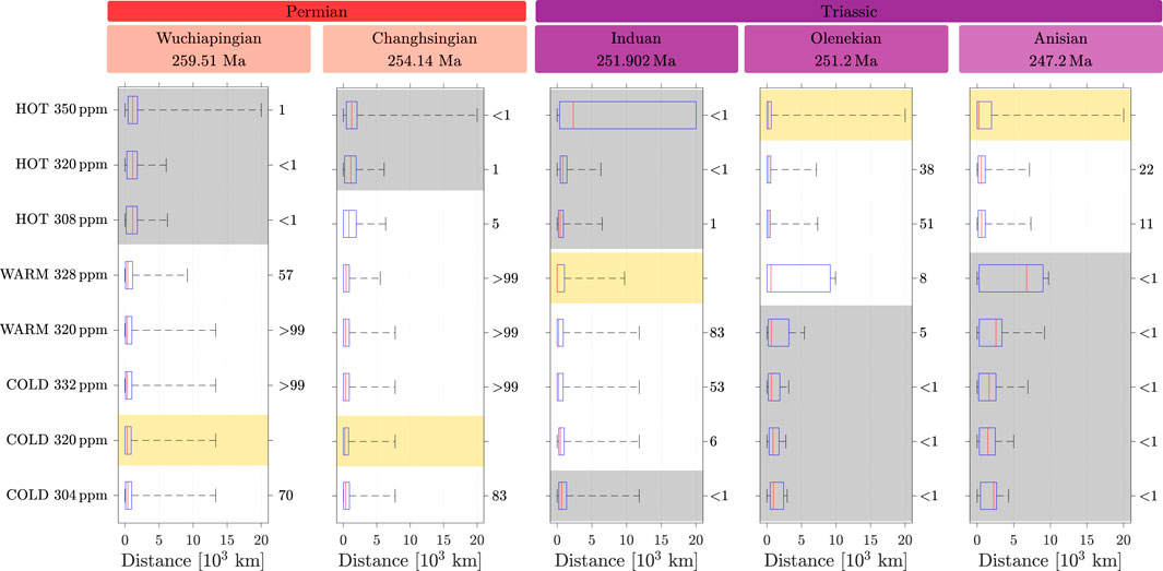
Figure 6. Whisker plot of the distances computed between each of the eight simulations and geological records for the five stages. For each stage, the yellow area indicates the simulation minimizing the median distance. The numbers on the right correspond to the $p$-values [%] of the difference between each distribution and the one highlighted in yellow. When rounding with 0 digits leads to 100% (resp. 0%), the notation $>99\%$ (resp. $<1\%$) is used instead. Gray areas indicate statistically significant differences. In this figure, temperate forbland biome is included in the cold temperate major biome (case 1).

For the Induan, the median in the warm-state simulation with 328 ppm is lower than that for the other simulations and is statistically different from the whole hot state and the lower edge of the cold-state branch.

For the Olenekian and the Anisian, the hot state at 350 ppm minimizes the median but is not significantly different from the same attractor with other atmospheric content of ${\text{CO}}_2$. For the Olenekian, the difference with the warm state at 328 ppm is also non-significant. However, in both cases, the hot state differs from the cold state, which can thus be excluded.

3.4 Robustness of the results against the classification of the temperate forbland biome

The classification of temperate forbland into cold temperate is questionable, as discussed in Section 2.3. In this study, we test the robustness of the results against the classification of this biome by including it in the desert major biome (case 2) instead of cold temperate (case 1).

3.4.1 Case 2: test on the mean values

The statistical analysis of the mean values is shown in Figure 7; Supplementary Table S3. The Wuchiapingian, Changhsingian, and Induan stages show better alignment between the geological records and cold and warm attractors. This tendency was already observed in the Lopingian, with the earlier classification of temperate forbland in the cold temperate major biome (case 1). However, the Induan did not display a clear tendency in favor of the hot or cold state in the previous analysis.

Figure 7

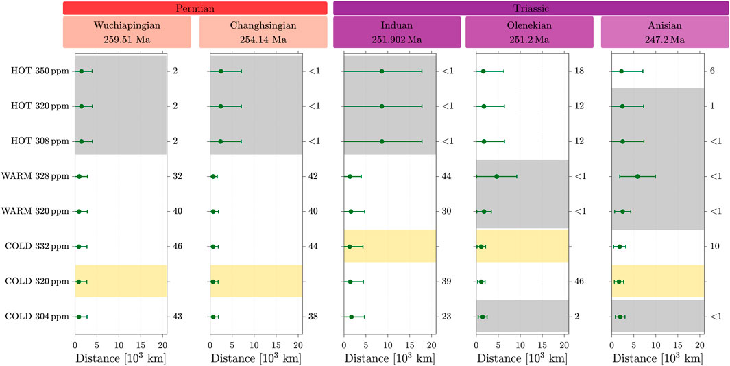
Figure 7. Same as Figure 5, except that the temperate forbland biome is included in the desert major biome (case 2).

In contrast, the results for both the Olenekian and Anisian stages do not differentiate the hot from the cold state. Although the minimal $\bar{d}$ is observed for the cold-state simulations in both cases, the hot state is not significantly different. For the Olenekian, the cold states with 320 ppm and 332 ppm and the entire hot-state branch cannot be excluded. For the Anisian, the upper cold-state branch and the hot state at 350 ppm match the data comparably well.

Therefore, in the mean test, this alternative classification (case 2) is less effective in distinguishing between the attractors compared to the previous option (case 1).

3.4.2 Case 2: test on the median values

The $p$-values for the test on the medians are reported in Figure 8 and detailed in Supplementary Table S4. As for the case with temperate forbland included in the cold temperate major biome, the statistical test shows a better matching of the cold and warm states in both the Wuchiapingian and Changhsingian. In this case, the same holds true for the Induan, where the cold state with 304 ppm is also significantly different from the other cold states.

Figure 8

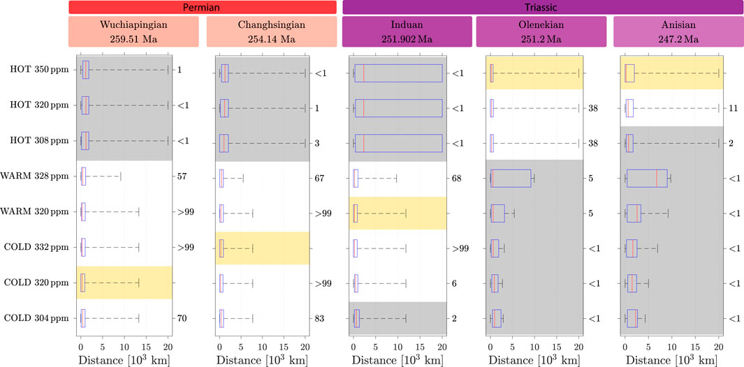
Figure 8. Same as Figure 6, except that the temperate forbland biome is included in the desert major biome (case 2).

For the Olenekian, the hot state with 350 ppm minimizes the median and is comparable to the other positions along the branch. In comparison with the case where temperate forbland is included in the cold temperate major biome, the hot state is favored here over the warm state at 328 ppm. For the Anisian, hot states at 320 ppm and 350 ppm match the vegetation pattern and are significantly different from the other simulations.

4 Summary and conclusion

The increasing temperatures observed between the Lopingian and Middle Triassic (Joachimski et al., 2012) are associated with a transition in the vegetation patterns reported by plant macrofossils (Nowak et al., 2020). We compared the changes over time in macrofossil assemblages to modeled biomes obtained from a series of climate simulations around the Permian–Triassic boundary, which revealed the existence of three alternative steady states with SATs differing by approximately 10$°$C (Ragon et al., 2024) (see Figure 1B).

The classification of the temperate forbland biome from the BIOME 4 vegetation model is ambiguous; therefore, two cases have been tested by including it either in cold temperate or desert major biomes. Its classification does not change the results for the Lopingian but has a larger impact on the Early Triassic, for which the presence of the cold temperate major biome in hot-state simulations is fully dependent on the assignment of the temperate forbland biome. The outlier values resulting from the absence of the cold temperate major biome in the hot-state simulations highly impact the mean values. However, the median is less sensitive to the outliers and, thus, to the classification of a particular biome, making the test on median values more robust and conclusive than the test on mean values.

The overall results are summarized in Figure 9 and show that the Lopingian matches well with both the cold and warm states in all tests. The early Middle Triassic (Anisian) is marked by the stabilization of the climate, as reported by ${\delta }^{13}$C isotope ratios (Payne et al., 2004). In our study, the vegetation distribution simulated for the hot state matches the fossil records of both the Anisian and Olenekian, in accordance with the stabilization of the vegetation patterns observed in the macrofossil collection in Nowak et al. (2020). The statistical tests show a significant difference between the hot and the warm/cold states, except the test on the mean values when temperate forbland is included in the desert major biome (case 2), for which the cold state cannot be completely excluded. This discontinuity, together with the fact that the mean value is more sensitive to outliers, leads us to consider this test as inconsistent and preferentially include the temperate forbland in the cold temperate major biome rather than in desert.

Figure 9

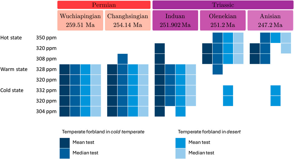
Figure 9. For each stage, the simulations that cannot be excluded from the data are highlighted in blue. The four statistical tests performed are shown from left to right (darker to lighter blue): test on mean and median values for temperate forbland included in the cold temperate major biome (case 1) and test on mean and median values for temperate forbland included in the desert major biome (case 2).

During the Induan, three tests out of four are in favor of a cold or warm state, whereas the remaining one is not conclusive (see Figure 9). Isotope ratios of ${\delta }^{13}C$ and ${\delta }^{18}O$ recorded oscillations during both the Induan and Olenekian, at shorter timescales than the age resolution considered in this study (Galfetti et al., 2007a; Romano et al., 2013; Goudemand et al., 2019; Widmann et al., 2020). These oscillations could be responsible for the equivocal signal for one attractor or another in the vegetation patterns of the Induan. However, the concordance of the Olenekian records with the hot state is more robust. Possible explanations for this difference can include i) oscillations between the hot and cold states for both the Induan and Olenekian but with more time spent in the hot state during the Olenekian; ii) a better preservation of macrofossils due to the (re-)establishment of wet biomes corresponding to the hot attractor; or iii) a possible bias in sampling. Sampling biases for the Early Triassic are highly likely, as discussed for example in Nowak et al. (2019). An alternative explanation for the unclear signal during the Induan might be related to its duration ($\sim$700 kyr), much shorter than the other stages; this shorter timeframe may have prevented the vegetation from stabilizing since ${\delta }^{13}C$ oscillations during this time interval were substantial, and palynological records indicate repeated disruptions affecting the floras during the Early Triassic (e. g.,Hochuli et al., 2016).

The warm state has a narrow, stable branch and cannot be reached through bifurcation-induced tipping from the other attractors (Ragon et al., 2024). Moreover, in all conditions, it is indistinguishable from at least one of the other attractors. Thus, it is relevant to focus on the two robust attractors, the hot and cold states, for the interpretation of the results.

In general, the results presented in this study on changes in the vegetation distribution over time suggest a transition from the cold attractor in the Lopingian to the hot attractor in the latest Early Triassic and early Middle Triassic, with a transient phase in the earliest Triassic (Induan) (see Figure 10). This study provides the most direct comparison to date between the Permian–Triassic plant fossil assemblages and climate simulations. The possibility of discriminating between attractors at the stage level highlights the relevance of using the multistability framework to describe the climatic variations recorded around the Permian–Triassic boundary.

Figure 10

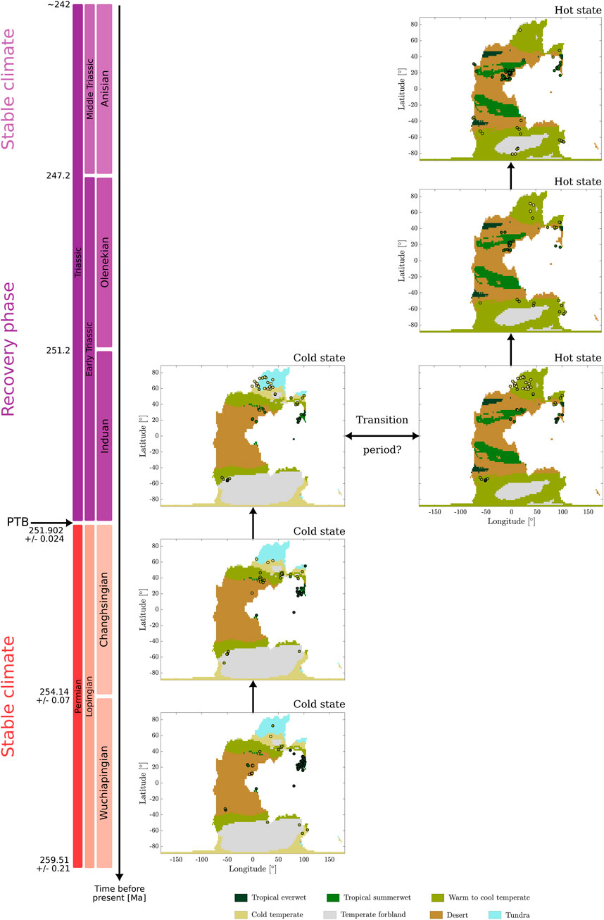
Figure 10. Summary of the comparison between the vegetation distribution associated with macrofossil records from the late Permian to the Early Triassic (Nowak et al., 2020) and the simulated climatic attractors, obtained using an offline coupling between the MITgcm and BIOME4 models, as described by Ragon et al. (2024).

Data availability statement

The original contributions presented in the study are included in the article/Supplementary Material; further inquiries can be directed to the corresponding author.

Author contributions

CR: methodology, writing–original draft, writing–review and editing, formal analysis, and visualization. CV: supervision, validation, and writing–review and editing. JK: supervision, validation, writing–review and editing, and methodology. HN: validation and writing–review and editing. EK: validation and writing–review and editing. MB: validation, writing–review and editing, conceptualization, funding acquisition, methodology, supervision, and writing–original draft.

Funding

The author(s) declare that financial support was received for the research, authorship, and/or publication of this article. We acknowledge the financial support from the Swiss National Science Foundation (Sinergia Project No. CRSII5_180253).

Acknowledgments

The authors thank all the Sinergia project members (PaleoC4, https://www.unige.ch/paleoc4/) and Emmanuel Castella for useful discussions. The simulations were performed on the Baobab and Yggdrasil clusters at the University of Geneva.

Conflict of interest

The authors declare that the research was conducted in the absence of any commercial or financial relationships that could be construed as a potential conflict of interest.

Generative AI statement

The author(s) declare that no Generative AI was used in the creation of this manuscript.

Publisher’s note

All claims expressed in this article are solely those of the authors and do not necessarily represent those of their affiliated organizations, or those of the publisher, the editors and the reviewers. Any product that may be evaluated in this article, or claim that may be made by its manufacturer, is not guaranteed or endorsed by the publisher.

Supplementary material

The Supplementary Material for this article can be found online at: https://www.frontiersin.org/articles/10.3389/feart.2025.1520846/full#supplementary-material

References

Adcroft, A., Campin, J.-M., Hill, C., and Marshall, J. (2004). Implementation of an atmosphere ocean general circulation model on the expanded spherical cube. Mon. Weather Rev. 132, 2845–2863. doi:10.1175/MWR2823.1

CrossRef Full Text | Google Scholar

Ashwin, P., Wieczorek, S., Vitolo, R., and Cox, P. (2012). Tipping points in open systems: bifurcation, noise-induced and rate-dependent examples in the climate system. Philosophical Trans. R. Soc. A Math. Phys. Eng. Sci. 370, 1166–1184. doi:10.1098/rsta.2011.0306

PubMed Abstract | CrossRef Full Text | Google Scholar

Bouyer, J. (1996). Méthodes statistiques: médecine-biologie (Estem).

Google Scholar

Brunetti, M., and Ragon, C. (2023). Attractors and bifurcation diagrams in complex climate models. Phys. Rev. E 107, 054214. doi:10.1103/PhysRevE.107.054214

PubMed Abstract | CrossRef Full Text | Google Scholar

Bucur, I. I., Rigaud, S., Del Piero, N., Fucelli, A., Heerwagen, E., Peybernes, C., et al. (2020). Upper triassic calcareous algae from the panthalassa ocean. Riv. Ital. Paleontol. Stratigr. 126. doi:10.13130/2039-4942/13681

CrossRef Full Text | Google Scholar

Burgess, S. D., Muirhead, J. D., and Bowring, S. A. (2017). Initial pulse of Siberian Traps sills as the trigger of the end-Permian mass extinction. Nat. Commun. 8, 164. doi:10.1038/s41467-017-00083-9

PubMed Abstract | CrossRef Full Text | Google Scholar

Callegaro, S., Svensen, H. H., Neumann, E. R., Polozov, A., Jerram, D. A., Deegan, F., et al. (2021). Geochemistry of deep Tunguska Basin sills, Siberian Traps: correlations and potential implications for the end-Permian environmental crisis. Contributions Mineralogy Petrology 176, 49. doi:10.1007/s00410-021-01807-3

CrossRef Full Text | Google Scholar

Chablais, J., Martini, R., Kobayashi, F., Stampfli, G. M., and Onoue, T. (2011). Upper Triassic foraminifers from Panthalassan carbonate buildups of Southwestern Japan and their paleobiogeographic implications. Micropaleontology 57, 93–124.

Google Scholar

Chu, D., Grasby, S. E., Song, H., Corso, J. D., Wang, Y., Mather, T. A., et al. (2020). Ecological disturbance in tropical peatlands prior to marine Permian-Triassic mass extinction. Geology 48, 288–292. doi:10.1130/G46631.1

CrossRef Full Text | Google Scholar

Cohen, K., Finney, S., Gibbard, P., and Fan, J. (2013). The ics international chronostratigraphic chart. Episodes 36, 199–204. doi:10.18814/epiiugs/2013/v36i3/002

CrossRef Full Text | Google Scholar

Davydov, V. (2021). Tunguska сoals, siberian sills and the permian-triassic extinction. Earth-Science Rev. 212, 103438. doi:10.1016/j.earscirev.2020.103438

CrossRef Full Text | Google Scholar

Feudel, U. (2023). Rate-induced tipping in ecosystems and climate: the role of unstable states, basin boundaries and transient dynamics. Nonlinear Process. Geophys. Discuss. 2023, 1–29. doi:10.5194/npg-2023-7

CrossRef Full Text | Google Scholar

Fielding, C. R., Frank, T. D., McLoughlin, S., Vajda, V., Mays, C., Tevyaw, A. P., et al. (2019). Age and pattern of the southern high-latitude continental end-Permian extinction constrained by multiproxy analysis. Nat. Commun. 10, 385. doi:10.1038/s41467-018-07934-z

PubMed Abstract | CrossRef Full Text | Google Scholar

Galfetti, T., Bucher, H., Ovtcharova, M., Schaltegger, U., Brayard, A., Brühwiler, T., et al. (2007a). Timing of the Early Triassic carbon cycle perturbations inferred from new U–Pb ages and ammonoid biochronozones. Earth Planet. Sci. Lett. 258, 593–604. doi:10.1016/j.epsl.2007.04.023

CrossRef Full Text | Google Scholar

Galfetti, T., Hochuli, P. A., Brayard, A., Bucher, H., Weissert, H., and Vigran, J. O. (2007b). Smithian-Spathian boundary event: evidence for global climatic change in the wake of the end-Permian biotic crisis. Geology 35, 291–294. doi:10.1130/G23117A.1

CrossRef Full Text | Google Scholar

Ghil, M., and Lucarini, V. (2020). The physics of climate variability and climate change. Rev. Mod. Phys. 92, 035002. doi:10.1103/RevModPhys.92.035002

CrossRef Full Text | Google Scholar

Goudemand, N., Romano, C., Leu, M., Bucher, H., Trotter, J. A., and Williams, I. S. (2019). Dynamic interplay between climate and marine biodiversity upheavals during the early Triassic Smithian -Spathian biotic crisis. Earth-Science Rev. 195, 169–178. doi:10.1016/j.earscirev.2019.01.013

CrossRef Full Text | Google Scholar

Gradstein, S., and Kerp, H. (2012). “Chapter 12 - a brief history of plants on earth,” in The geologic time scale. Editors F. M. Gradstein, J. G. Ogg, M. D. Schmitz, and G. M. Ogg (Boston: Elsevier), 233–237. doi:10.1016/B978-0-444-59425-9.00012-3

CrossRef Full Text | Google Scholar

Haxeltine, A., and Prentice, I. C. (1996). BIOME3: an equilibrium terrestrial biosphere model based on ecophysiological constraints, resource availability, and competition among plant functional types. Glob. Biogeochem. Cycles 10, 693–709. doi:10.1029/96GB02344

CrossRef Full Text | Google Scholar

Hochuli, P. A., Hermann, E., Vigran, J. O., Bucher, H., and Weissert, H. (2010). Rapid demise and recovery of plant ecosystems across the end-permian extinction event. Glob. Planet. Change 74, 144–155. doi:10.1016/j.gloplacha.2010.10.004

CrossRef Full Text | Google Scholar

Hochuli, P. A., Sanson-Barrera, A., Schneebeli-Hermann, E., and Bucher, H. (2016). Severest crisis overlooked—worst disruption of terrestrial environments postdates the Permian–Triassic mass extinction. Sci. Rep. 6, 28372. doi:10.1038/srep28372

PubMed Abstract | CrossRef Full Text | Google Scholar

Joachimski, M. M., Lai, X., Shen, S., Jiang, H., Luo, G., Chen, B., et al. (2012). Climate warming in the latest Permian and the Permian–Triassic mass extinction. Geology 40, 195–198. doi:10.1130/G32707.1

CrossRef Full Text | Google Scholar

Kaplan, J. O. (2001). Geophysical applications of vegetation modeling. Tech. Rep.

Google Scholar

Kaplan, J. O., Bigelow, N. H., Prentice, I. C., Harrison, S. P., Bartlein, P. J., Christensen, T. R., et al. (2003). Climate change and arctic ecosystems: 2. modeling, paleodata-model comparisons, and future projections. J. Geophys. Res. Atmos. 108. doi:10.1029/2002JD002559

CrossRef Full Text | Google Scholar

Le Houedec, S., Fucelli, A., Peyrotty, G., Vérard, C., and Martini, R. (2024). Does the panthalassa ocean circulation really rely on single hemispheric gyre? New insight from Nd isotopes from open ocean late triassic terranes. SSRN Prepr. doi:10.2139/ssrn.4939666

CrossRef Full Text | Google Scholar

Looy, C. V., Twitchett, R. J., Dilcher, D. L., Cittert, J. H. A. V. K.-V., and Visscher, H. (2001). Life in the end-Permian dead zone. Proc. Natl. Acad. Sci. 98, 7879–7883. doi:10.1073/pnas.131218098

PubMed Abstract | CrossRef Full Text | Google Scholar

Margazoglou, G., Grafke, T., Laio, A., and Lucarini, V. (2021). Dynamical landscape and multistability of a climate model. Proc. R. Soc. A Math. Phys. Eng. Sci. 477, 20210019. doi:10.1098/rspa.2021.0019

PubMed Abstract | CrossRef Full Text | Google Scholar

Marshall, J., Adcroft, A., Campin, J.-M., Hill, C., and White, A. (2004). Atmosphere–ocean modeling exploiting fluid isomorphisms. Mon. Weather Rev. 132, 2882–2894. doi:10.1175/MWR2835.1

CrossRef Full Text | Google Scholar

Marshall, J., Adcroft, A., Hill, C., Perelman, L., and Heisey, C. (1997a). A finite-volume, incompressible Navier Stokes model for studies of the ocean on parallel computers. J. Geophys. Res. 102, 5753–5766. doi:10.1029/96JC02775

CrossRef Full Text | Google Scholar

Marshall, J., Hill, C., Perelman, L., and Adcroft, A. (1997b). Hydrostatic, quasi-hydrostatic, and nonhydrostatic ocean modeling. J. Geophys. Res. 102, 5733–5752. doi:10.1029/96JC02776

CrossRef Full Text | Google Scholar

Mays, C., and McLoughlin, S. (2022). End-Permian burnout: the role of Permian-Triassic wildfires in extinction, carbon cycling, and environmental change in Eastern Gondwana. PALAIOS 37, 292–317. doi:10.2110/palo.2021.051

CrossRef Full Text | Google Scholar

Mays, C., Vajda, V., Frank, T. D., Fielding, C. R., Nicoll, R. S., Tevyaw, A. P., et al. (2019). Refined Permian–Triassic floristic timeline reveals early collapse and delayed recovery of south polar terrestrial ecosystems. GSA Bull. 132, 1489–1513. doi:10.1130/B35355.1

CrossRef Full Text | Google Scholar

Mays, C., Vajda, V., and McLoughlin, S. (2021). Permian–Triassic non-marine algae of Gondwana—distributions, natural affinities and ecological implications. Earth-Science Rev. 212, 103382. doi:10.1016/j.earscirev.2020.103382

CrossRef Full Text | Google Scholar

Mood, A. M. (1950). Introduction to the theory of statistics. New York, NY, US: McGraw-Hill.

Google Scholar

Nowak, H., Schneebeli-Hermann, E., and Kustatscher, E. (2019). No mass extinction for land plants at the permian–triassic transition. Nat. Commun. 10, 384. doi:10.1038/s41467-018-07945-w

PubMed Abstract | CrossRef Full Text | Google Scholar

Nowak, H., Vérard, C., and Kustatscher, E. (2020). Palaeophytogeographical patterns across the permian–triassic boundary. Front. Earth Sci. 8. doi:10.3389/feart.2020.613350

CrossRef Full Text | Google Scholar

Payne, J. L., Lehrmann, D. J., Wei, J., Orchard, M. J., Schrag, D. P., and Knoll, A. H. (2004). Large perturbations of the carbon cycle during recovery from the end-permian extinction. Science 305, 506–509. doi:10.1126/science.1097023

PubMed Abstract | CrossRef Full Text | Google Scholar

Peyrotty, G., Brigaud, B., and Martini, R. (2020). δ¹⁸O, δ¹³C, trace elements and REE in situ measurements coupled with U–Pb ages to reconstruct the diagenesis of upper triassic atoll-type carbonates from the Panthalassa Ocean. Mar. Petroleum Geol. 120, 104520. doi:10.1016/j.marpetgeo.2020.104520

CrossRef Full Text | Google Scholar

Ragon, C., Vérard, C., Kasparian, J., and Brunetti, M. (2024). Alternative climatic steady states near the Permian-Triassic Boundary. Sci. Rep. 14, 26136. doi:10.1038/s41598-024-76432-8

PubMed Abstract | CrossRef Full Text | Google Scholar

Raup, D. M., and Sepkoski, J. J. (1982). Mass extinctions in the marine fossil record. Science 215, 1501–1503. doi:10.1126/science.215.4539.1501

PubMed Abstract | CrossRef Full Text | Google Scholar

Renne, P. R., and Basu, A. R. (1991). Rapid eruption of the siberian Traps flood basalts at the permo-triassic boundary. Science 253, 176–179. doi:10.1126/science.253.5016.176

PubMed Abstract | CrossRef Full Text | Google Scholar

Renne, P. R., Black, M. T., Zichao, Z., Richards, M. A., and Basu, A. R. (1995). Synchrony and causal relations between permian-triassic boundary crises and siberian flood volcanism. Science 269, 1413–1416. doi:10.1126/science.269.5229.1413

PubMed Abstract | CrossRef Full Text | Google Scholar

Retallack, G. J. (1999). Postapocalyptic greenhouse paleoclimate revealed by earliest Triassic paleosols in the Sydney Basin, Australia. GSA Bull. 111, 52–70. doi:10.1130/0016-7606(1999)111⟨0052:PGPRBE⟩2.3

CrossRef Full Text | Google Scholar

Rogger, J., Judd, E. J., Mills, B. J. W., Goddéris, Y., Gerya, T. V., and Pellissier, L. (2024). Biogeographic climate sensitivity controls earth system response to large igneous province carbon degassing. Science 385, 661–666. doi:10.1126/science.adn3450

PubMed Abstract | CrossRef Full Text | Google Scholar

Romano, C., Goudemand, N., Vennemann, T. W., Ware, D., Schneebeli-Hermann, E., Hochuli, P. A., et al. (2013). Climatic and biotic upheavals following the end-Permian mass extinction. Nat. Geosci. 6, 57–60. doi:10.1038/ngeo1667

CrossRef Full Text | Google Scholar

Schneebeli-Hermann, E. (2020). Regime shifts in an early triassic subtropical ecosystem. Front. Earth Sci. 8. doi:10.3389/feart.2020.588696

CrossRef Full Text | Google Scholar

Sibik, S., Edmonds, M., Maclennan, J., and Svensen, H. (2015). Magmas erupted during the main pulse of siberian Traps volcanism were volatile-poor. J. Petrology 56, 2089–2116. doi:10.1093/petrology/egv064

CrossRef Full Text | Google Scholar

Stanley, S. M. (2016). Estimates of the magnitudes of major marine mass extinctions in earth history, Proc. Natl. Acad. Sci. U. S. A. 113, E6325–E6334. doi:10.1073/pnas.1613094113

PubMed Abstract | CrossRef Full Text | Google Scholar

Svensen, H. H., Frolov, S., Akhmanov, G. G., Polozov, A. G., Jerram, D. A., Shiganova, O. V., et al. (2018). Sills and gas generation in the siberian Traps. Philosophical Trans. R. Soc. A Math. Phys. Eng. Sci. 376, 20170080. doi:10.1098/rsta.2017.0080

PubMed Abstract | CrossRef Full Text | Google Scholar

Vajda, V., McLoughlin, S., Mays, C., Frank, T. D., Fielding, C. R., Tevyaw, A., et al. (2020). End-Permian (252 Mya) deforestation, wildfires and flooding—an ancient biotic crisis with lessons for the present. Earth Planet. Sci. Lett. 529, 115875. doi:10.1016/j.epsl.2019.115875

CrossRef Full Text | Google Scholar

Vérard, C. (2019). Panalesis: towards global synthetic palaeogeographies using integration and coupling of manifold models. Geol. Mag. 156, 320–330. doi:10.1017/s0016756817001042

CrossRef Full Text | Google Scholar

Vérard, C. (2021). 888–444 Ma global plate tectonic reconstruction with emphasis on the formation of Gondwana. Front. Earth Sci. 9. doi:10.3389/feart.2021.666153

CrossRef Full Text | Google Scholar

Walter, H. (2012). Vegetation of the earth and ecological systems of the geo-biosphere. Springer Science and Business Media.

Google Scholar

Widmann, P., Bucher, H., Leu, M., Vennemann, T., Bagherpour, B., Schneebeli-Hermann, E., et al. (2020). Dynamics of the largest carbon isotope excursion during the early triassic biotic recovery. Front. Earth Sci. 8. doi:10.3389/feart.2020.00196

CrossRef Full Text | Google Scholar

Zar, J. (2010). Biostatistical Analysis. 5th Edition. Upper Saddle River: Prentice-Hall/Pearson.

Google Scholar

Ziegler, A. M. (1990). Phytogeographic patterns and continental configurations during the Permian Period. Geol. Soc. Lond. Memoirs 12, 363–379. doi:10.1144/GSL.MEM.1990.012.01.35

CrossRef Full Text | Google Scholar