Multidecadal estimation of hydrological contribution and glacier mass balance in the semi-arid Andes based on physically based modeling and geodetic mass balance

Glaciers are of paramount importance in diverse environments, and due to the accelerated retreat experienced in recent decades, efforts have intensified to achieve a comprehensive understanding of key variables such as mass balance and glacial melting. However, the scarcity of data in regions that are difficult to access, such as the Andes Cordillera, hinders reliable glaciological studies of the historical period. This study examined the mass balance and melting dynamics of the Universidad Glacier, the largest in the semi-arid Andes, from 1955 to 2020, using the physically based Cold Regions Hydrological Model (CRHM). The model was calibrated with geodetic mass balance estimates available between 1955 and 2020 and evaluated against on-site observations available between 2012 and 2014. Change point analysis revealed three contrasting periods of mass balance evolution: significant mass loss for the periods 1955–1971 and 2006–2020 and near-equilibrium mass balance from 1971 to 2006. These loss and gain periods align with the negative phases of the Pacific Decadal Oscillation (PDO) and the positive ENSO (El Niño) events, respectively. Simulated runoff from glacier melt showed a positive trend of 8% per decade since 1971. Calibrated and uncalibrated versions of the model showed similar temporal variability, but cumulative mass balance differed significantly. The model calibrated from 1955 to 2020 had a minimal overestimation of 0.1% in mass loss and slightly improved the representation of the annual albedo. Relative to this best-performing model, the model calibrated with geodetic mass balance estimates from 2000 to 2020 overestimated mass loss by 25%, whereas the uncalibrated model overestimated mass balance by 62%. Physically based modeling with parameters adjusted based on field observations is adequate to reproduce the most salient features of MB interannual variability. However, long-term projections may diverge significantly, and albedo parameterizations, including its spatial and temporal evolution throughout a glacier surface, are an avenue for future research.

Introduction

With a few exceptions, glaciers worldwide are experiencing rapid retreat. In high-mountain regions, this process has consequences for water supply, ecological function, and geohazards. In the extratropical Andes region of Chile (25°–35°S), snowmelt serves as the main source of freshwater by volume, but glacier melt contributes significantly, especially during late summer and in drought years (Ayala et al., 2020). Studies using remote-sensing techniques have consistently recorded glacier retreat in the Chilean Andes, which has affected primarily debris-free or clean glaciers (Masiokas et al., 2020; Barcaza et al., 2017). Through geodetic mass balance estimation, Dussaillant et al. (2019) found that glaciers in the extratropical Andes (25°–35°S) experienced a near-equilibrium mass balance between 2000 and 2009 but significant mass losses between 2009 and 2018. The latter period overlaps with the so-called 2010 Chile Megadrought (Garreaud et al., 2017), which was characterized by higher temperatures, moderate but persistent annual precipitation deficits, and some of the driest years on record.

Developing adequate strategies for adaptation to cryosphere changes, such as those experienced by extratropical Andean glaciers, requires reliable projections of ice mass evolution under climate scenarios. Numerical models can be valuable tools if they can reliably represent the sequence of hydrological stores and fluxes in high mountain environments. Among the modeling decisions required, the snow and ice melt scheme is one of the most relevant. The degree-day index method requires only temperature and precipitation as meteorological inputs and has proven useful for regional- or global-scale glacier models such as GloGEM (Huss and Hock, 2018) and the open global glacier model (Maussion et al., 2019). Some models modify the degree-day index by explicitly considering radiation inputs (Pellicciotti et al., 2014). This approach has been employed in the TOPKAPI-ETH model (Fatichi et al., 2015; Ragettli et al., 2016), allowing for improved performance of a degree-day model by adding only one meteorological predictor (Pellicciotti et al., 2014). The energy balance method estimates melt rates based on the available energy at the glacier’s surface from exchange with the atmosphere. This approach requires a larger amount of meteorological data, including air temperature, precipitation, and net shortwave and longwave radiation. Energy balance models can be used to develop estimates at the watershed, glacier, or point scale. Examples of modeling platforms using this approach include DHSVM-GDN (Naz et al., 2014), COSIPY v1.3 (Sauter et al., 2020), and DEBAM (Hock and Holmgren, 2005; Kinnard et al., 2022). Pradhananga and Pomeroy (2022) added a glacier module to the Cold Regions Hydrological Model (CRHM-glacier), an evolution that includes a module for ice and firn mass and energy balances and combines them with the original model components described in Pomeroy et al. (2007). CRHM-glacier allows combining a physically based representation of glacier ablation with off-glacier hydrological modeling at the river basin scale, thus enabling the study of the contribution of glaciers to downstream hydrology. It has been applied to the Peyto Glacier in the Canadian Rockies (Aubry-Wake et al., 2022; Aubry-Wake and Pomeroy, 2023), providing diagnostics of hydrological controls of runoff production and change estimates for the future evolution of landscape and meteorological forcing.

Although parameters in physically based models are generally observable, some degree of calibration is needed because of the general scarcity of relevant observations in remote high-mountain areas. In recent years, the use of geodetic estimates obtained from satellite sensors or photogrammetry has significantly expanded the temporal and spatial coverage of glacier mass balance studies to nearly global coverage (Braithwaite and Hughes, 2020; Berthier et al., 2023; Hugonnet et al., 2021), and enabled the calibration and/or evaluation of glaciological models, particularly those based on temperature-index melt estimation (Barandun et al., 2022; Compagno et al., 2022; McCarthy et al., 2022; Li et al., 2023; Rounce et al., 2023). Most techniques for obtaining geodetic mass balances are only available after 2000 (Berthier et al., 2023). However, geodetic mass balances obtained from differences in digital elevation models generated using optical stereoscopic images provide the opportunity to undertake mass balance studies that span longer periods, including data from the 1960s.

In this study, we focus on the largest individual glacier in the extratropical Andes, the Universidad Glacier. We seek to complement the knowledge regarding the hydrological role and historical evolution of glaciers in the southern portion of this region, which receives comparatively higher annual precipitation than the glacierized catchments reported by Ayala et al. (2020) and Masiokas et al. (2016), with the aim of assessing the value of long-term geodetic mass balance estimates for model calibration and evaluation under a physically based framework. To this end, we employ the CRHM-glacier platform to represent the high-mountain river basin that contains the glacierized area and adjust the most sensitive parameters based on the subsets of geodetic mass balance estimates.

Study domain

Universidad Glacier (34°40'S, 70°20'W), located in the semi-arid Andes at the head of the Tinguiririca River, is the largest glacier north of Patagonia, with an area of 26.3 km² (Barcaza et al., 2017). The regional climate is highly seasonal, with most of the precipitation occurring during the winter months from May to September. The Universidad Glacier spans an altitudinal range of 2,482–4,970 m a.s.l. and has a predominant southeast orientation (Barcaza et al., 2017). The glacier comprises two sub-basins that function as accumulation zones. These two accumulation zones merge downstream of two icefalls, forming the glacier tongue. The presence of debris on the glacier tongue is discontinuous, with the upper part exhibiting ogives (Wilson et al., 2016). While there is a greater presence of detritus near the glacier terminus, it does not form a homogeneous and continuous layer, although the percentage of detritus cover in the lower zone has been increasing over the last decade due to low precipitation (Podgórsky et al., 2023). Figure 1 shows the location and geometric disposition of the glacier along with the locations of various station observations available for this study. The outline of the Tinguiririca River at the Los Briones stream gage, to which the flow from the glacierized catchment converges, is also shown.

Figure 1

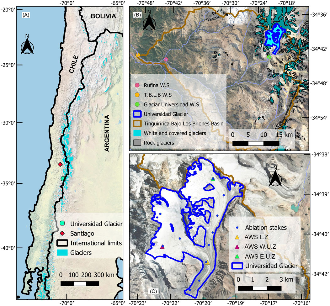
Figure 1. Study area and location of available station data. (A) Relative position of the Universidad Glacier with respect to Santiago de Chile. (B) Tinguiririca Bajo Los Briones (TBLB) Basin and location of the gauging station. In addition, the location of the Rufina (Rufina WS) and Universidad Glacier (Glaciar Universidad WS) weather stations were used to calculate precipitation gradients. (C) Limits of the Universidad Glacier (DGA, 2022), locations of automatic weather stations (AWS), and ablation stakes of Kinnard et al. (2018).

Methods

Universidad Glacier hydroglaciological model

The CRHM-glacier model structure for the glacial watershed is based on the framework presented by Pradhananga and Pomeroy (2022). CRHM is a physically based modeling platform that allows for the modular simulation of various processes related to snow accumulation, ablation, and runoff. In CRHM, the study area is discretized into hydrologic response units (HRUs), within which hydrological features are assumed to be spatially homogeneous. This approach enables a parsimonious representation of the spatial variability within the watershed and helps reduce computational time. The HRUs for the Universidad Glacier were defined based on topographic attributes and glacier boundaries. The glacier outline corresponds to 2018 and was obtained from the Public Glacier Inventory (Barcaza et al., 2017). Terrain topography was obtained from ASTER DEM (ASTER Science Team, 2019) and classified according to elevation (100-m bands), orientation (four directions), and slope (three classes between 0° and 90°), resulting in 55 HRUs, with an average size of 0.54 km². Figure 2 illustrates the topographic attributes of the glacier and the resulting HRUs.

Figure 2

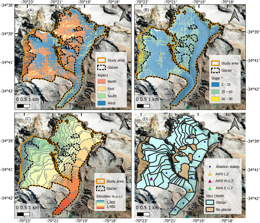
Figure 2. Topographic attributes for HRU discretization. (A) Aspect discretization. (B) Slope discretization. (C) Altitudinal discretization. (D) Resulting HRU discretization. The blue dots represent the ablation stakes of Kinnard et al. (2018), and the triangles represent the AWS of the same study.

Snowmelt for glacier and nonglacier HRUs was calculated using the SNOBAL module (Marks et al., 1998), which applies energy and mass conservation parameterizations to a two-layer snowpack. Melting of glacier ice and firn was calculated using an energy balance approach, as detailed by Pradhananga and Pomeroy (2022). Gravitational snow redistribution between HRUs was modeled based on Bernhardt and Schulz (2010) and implemented in the SWESlope module. The Prairie blowing snow module (PBSM) (Pomeroy, 1997; Pomeroy and Li, 2000) was used to calculate blowing snow transport and also accounted for blowing snow sublimation. The radiation inputs required for the snow and glacier melt modules were computed based on air temperature data. Incident shortwave radiation was obtained using the Annandale module (Annandale et al., 2002), updating the coefficient of the method to a value of 0.2 to match local pyranometer observations. Longwave radiation was estimated using the parameterization developed by Sicart et al. (2006) in the long Vt module.

In the CRHM-glacier model, the treatment of albedo differs for snow and firn/ice. For snow albedo, the model follows the dynamics presented by Verseghy (1991), whereby snow albedo (α_t) exhibits a linear decay for cold snow, while melting snow has an empirical exponential decay function, as described in Equation 1:

${\mathit{\alpha }}_{\mathit{t}}\left\{\begin{array}{l}{\mathit{\alpha }}_{\mathit{t}-\mathbf{1}}-\frac{∆\mathit{t}}{{\mathbf{a}}_{\mathbf{1}}},\mathbf{c}\mathbf{o}\mathbf{l}\mathbf{d}\mathbf{s}\mathbf{n}\mathbf{o}\mathbf{w}\\ \left({\mathit{\alpha }}_{\mathit{t}-\mathbf{1}}-{\mathit{\alpha }}_{\mathbf{min}}\right)*{\mathit{e}}^{-\frac{∆\mathit{t}}{{\mathbf{a}}_{\mathbf{2}}}}+{\mathit{\alpha }}_{\mathbf{min}},\mathbf{m}\mathbf{e}\mathbf{l}\mathbf{t}\mathbf{i}\mathbf{n}\mathbf{g}\mathbf{s}\mathbf{n}\mathbf{o}\mathbf{w}.\end{array}\right.(1)$

Furthermore, the snow albedo is refreshed based on the magnitude of snowfall, as shown in Equation 2:

${\mathit{\alpha }}_{\mathit{t}}={\mathit{\alpha }}_{\mathit{t}-\mathbf{1}}+\left({\mathit{\alpha }}_{\mathbf{max}}-{\mathit{\alpha }}_{\mathbf{t}-\mathbf{1}}\right)*\frac{{\mathbf{s}}_{\mathbf{f}}}{{\mathbf{s}}_{\mathbf{min}}},(2)$

where ${\mathrm{\alpha }}_{t-1}$ and ${\mathrm{\alpha }}_t$ are the albedo for the previous and current time steps, respectively. ${\mathrm{\alpha }}_{\max }$ and ${\mathrm{\alpha }}_{\min }$ are the maximum albedo of fresh snow and the minimum albedo of aged snow, respectively. ${\mathrm{s}}_{\mathrm{f}}$ is the amount of snowfall in the time step, ${\mathrm{s}}_{\min }$ is the minimum amount of snowfall required to refresh the albedo to ${\mathrm{\alpha }}_{\max },$ and ${\mathrm{a}}_1$ and ${\mathrm{a}}_{\mathbf{2}}$ are the time-decay parameters.

We assigned ${\mathrm{\alpha }}_{\max }$ based on daily snow albedo data derived from the MODIS products Terra Snow Cover Daily L3 Global 500 m (MOD10A1) and Aqua Snow Cover Daily L3 Global 500 m (MYD10A1) (Hall et al., 2002). By averaging the annual maximum snow albedo over the glacier for the period 2000–2020, we obtained a value of 0.90, which is consistent with automatic weather stations (AWS) observations reported by Kinnard et al. (2018). We derived the minimum snow albedo (${\mathrm{\alpha }}_{\min }$) and ice albedo from the albedo grids presented by Shaw et al. (2020), who examined the albedo of various glaciers in the central Chilean Andes (33–34ºS) using late summer Landsat scenes from 1986 to 2020. Their analysis revealed a negative albedo trend that was statistically correlated with annual precipitation. For the Universidad Glacier, the decreasing trend in ice albedo was −0.014 per decade. For the ice albedo parameter, we calculated the average albedo value for each HRU between 1991 and 2020 using the albedo grids generated by Shaw et al. (2020) and fitting a linear decay trend to these values. For the years prior to 1990, we applied fixed ice albedo values derived from the 1991 image. For the minimum snow albedo (${\mathrm{\alpha }}_{\min }$), we averaged the albedo values from late summer images for the pixels categorized as snow by Shaw et al. (2020), resulting in a minimum snow albedo of 0.35. This value was consistent with the AWS observations reported by Kinnard et al. (2018) and aligned with the March monthly mean albedo calculated for the Central Andes by Malmros et al. (2018).

The decay parameter ${\mathbf{a}}_{\mathbf{1}}$ was estimated from data obtained at the Valle Nevado cryosphere station, operated by the Universidad de Chile, and assigned a value of 34.72 days. For parameter ${\mathbf{a}}_{\mathbf{2}}$, we adopted a value of 13.9 days and set the value of ${\mathbf{s}}_{\mathbf{min}}$ to 1 mm, following the approach reported by Jara et al. (2021).

Ice flow was not explicitly calculated in the current version of CRHM-glacier. To distribute the ice thickness and avoid the unrealistic disappearance of ice in the lowest HRUs, we implemented the ∆h parameterization (Huss et al., 2010), which redistributes ice height changes along the glacier elevation range through an empirical approximation related to the glacier size and geometry. In our study, we obtained the elevation change data from Hugonnet et al. (2021) for the period 2000–2019. The elevation bands used in the parameterization correspond to the same 100-m intervals that were utilized for generating the HRUs (see Figure 2). CRHM-glacier does not compute changes in the geometry or area of the glacier. However, satellite data suggest that the Universidad Glacier experienced a relatively modest area loss of only 6% between 1945 and 2011 (DGA, 2011).

Meteorological forcings

The CRHM-glacier model requires a three-hourly series of precipitation, air temperature, wind speed, and relative humidity for the period 1955–2020. All inputs were obtained from ERA5-Land reanalysis according to the following procedure: three-hourly precipitation and daily maximum and minimum air temperature values were bias-corrected using the multivariate quantile mapping bias correction (MBCn) technique (Cannon, 2018) using the observation-based CR2MET gridded product (Boisier et al., 2016) as a reference. Both the ERA5-Land and CR2MET datasets were filtered to remove precipitation from days with values lower than 1 mm, which were deemed unrealistic and inconsistent with observational records.

Bias-corrected precipitation was then distributed from the pixel resolution to the model HRUs using a logarithmic altitudinal gradient (Equation 3) derived from the precipitation records at three weather stations operated by the Chilean Water Directorate (DGA), as shown in Figure 1 and Table 1. The logarithmic gradient was calibrated using precipitation observations from July 2018 to April 2020:

${\mathbf{P}}_{\mathbf{HRU}}=\left(\mathbf{0.33}*\mathbf{ln}\left(\mathbf{z}\right)-\mathbf{1.6}\right)*{\mathbf{P}}_{\mathbf{E}\mathbf{R}\mathbf{A}.\mathbf{B}\mathbf{C},}(3)$

where P_HRU is the HRU precipitation, z is the HRU elevation, and P_{ERA. BC} is the precipitation at the centroid of the bias-corrected ERA5-L and precipitation product grid cells.

Table 1

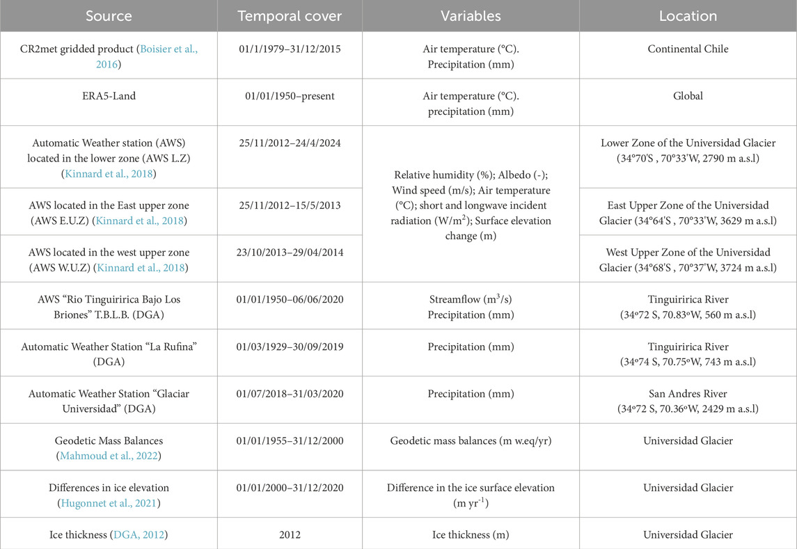
Table 1. Summary of the different data sources used.

Air temperature was spatially distributed to the model resolution using altitudinal gradients estimated from on-glacier AWS data. Three linear elevation gradients were derived. One gradient was determined for the eastern accumulation zone using the temperature data during the ablation period from December 2012 to May 2013. This resulted in a lapse rate of 5.5°C ± 1.0°C km⁻¹, which is consistent with that estimated by Bravo et al. (2017) for the same area. Another gradient was calculated for the western accumulation zone using temperature data from November 2013 to April 2014, which resulted in a sharper lapse rate of 7.6°C ± 0.9°C km⁻¹. The higher gradient in the western zone could be attributed to the exacerbation of the effect described by Bravo et al. (2017), involving the erosion of the katabatic boundary layer due to the advection of warm air from the extensive bare rock areas in the southeastern zone of the glacier situated between the tongue and the western accumulation zone valley.

Wind speed and relative humidity series for the hydroglaciological model were constructed using synthetic series based on the records from the AWS located in the lower part of the glacier, aggregated at 3-h intervals. The time series was calculated by considering an additive model with three components: seasonal, trend, and random. For each month of the year, an independent additive model was fitted to the three-hourly average values of wind speed and relative humidity. To distribute relative humidity across the glacier, an altitudinal gradient was calculated using the same procedure as that for temperature. For the eastern part of the glacier, the calculated altitudinal gradient was −10% km⁻¹. For the western part of the glacier, the gradient was −6.5% km⁻¹. We did not find a significant wind spatial pattern between the upper and lower AWS. Therefore, the same wind speed value obtained from the lower AWS was used for the entire glacier.

Mass balance

Historical glacier mass evolution was derived from changes in glacier elevations calculated by Hugonnet et al. (2021) and the geodetic mass balance data presented by Mahmoud et al. (2022). Hugonnet et al. (2021) utilized stereo images from the Advanced Spaceborne Thermal Emission and Reflection Radiometer (ASTER) to derive glacier surface elevation changes. They computed these changes for four 5-year periods: 2000–2004, 2005–2009, 2010–2014, and 2015–2019. In contrast, Mahmoud et al. (2022) calculated mass balance based on historical aerial photogrammetry data collected by the Aerial Photogrammetry Service (SAF) and Military Geographic Institute of Chile (IGM) in the years 1955, 1985, and 1997 to create digital elevation models, later co-registered with the SRTM Digital Elevation Model. We incorporated the mass balance estimates for two periods: 1955–1985 and 1985–1997. To evaluate the model, we used glaciological mass balance measurements available from 2012 to 2014 (Kinnard et al., 2018). Ice thickness was obtained from a study conducted by the Chilean Water Directorate in 2011 using radio echo sounding (DGA, 2012).

Model calibration and evaluation

Although the physically based nature of the CRHM platform allows most parameter values to be assigned from direct observations, we carried out a calibration exercise to evaluate the impact of adjusting model outputs to different periods of geodetic mass balance retrievals. A first model was uncalibrated (unc) using default parameters suggested by Pradhananga and Pomeroy (2022) and values estimated from local data, as described in previous sections. A second model (crec) was calibrated using geodetic mass balance estimates from 2000 to 2020 (Hugonnet et al., 2021). This period is characterized by higher glacier mass loss, warmer temperatures, and the occurrence of the Chile megadrought since 2010. A third model (cext) was calibrated using mass balances from 1955 to 2020, incorporating geodetic mass balances from Mahmoud et al. (2022) and Hugonnet et al. (2021). The period from 1955 to 2000 covers greater hydroclimatic variability, including some shorter drought periods compared to the more recent megadrought, along with a warming temperature trend (Burger et al., 2018). Figure 3A shows the geodetic mass balance values per period together with the annual precipitation and temperature series. The models were calibrated using the shuffled complex evolution (SCE) global optimization method (Duan et al., 1992) implemented in the rtop package. The objective function for the SCE algorithm was the root-mean-square error (RMSE) of the mass balance for each period (Equation 4), considering the geodetic mass balances as reference:

$\mathbf{R}\mathbf{M}\mathbf{S}\mathbf{E}\hspace{0.17em}\mathbf{M}.\mathbf{B}=\sqrt{\frac{\mathbf{1}}{\mathbf{m}}{\displaystyle \sum _{\mathbf{j}=\mathbf{i}}^{\mathbf{m}}}\left({\Delta \mathbf{h}}_{\mathbf{r}\mathbf{e}\mathbf{f}\mathbf{i}}-{\Delta \mathbf{h}}_{\mathbf{s}\mathbf{i}\mathbf{m}\mathbf{i}}\right),}(4)$

where ∆h_ref,i is the geodetic mass balance of the period and ∆h_{sim i} is the mass balance calculated by the model.

Figure 3

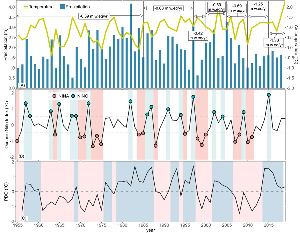
Figure 3. Time series of local and regional climate variables. (A) Average annual temperature and precipitation over the glaciers. The arrows and vertical lines indicate the average mass balance of the Universidad Glacier over the delimited periods. The sources are listed in Table 1. (B) Annual series of the Oceanic Niño Index (ONI), where light blue stripes correspond to Niño years and red stripes correspond to Niña years. (C) Pacific decadal oscillation (PDO) index.

Parameters for calibration were selected based on the distributed evaluation of local sensitivity analysis (DELSA) method (Rakovec et al., 2014). DELSA uses “local” derivative-based methods to estimate parameter sensitivity based on the response in the gradient of the model output or performance index. The sensitivity of the parameters is assessed across the parameter space by selecting different points using a Latin hypercube. We chose the DELSA method due to its capability to scan the parameter space at a relatively low computational cost. Table 2 shows the subset of model parameters included in the DELSA procedure.

Table 2

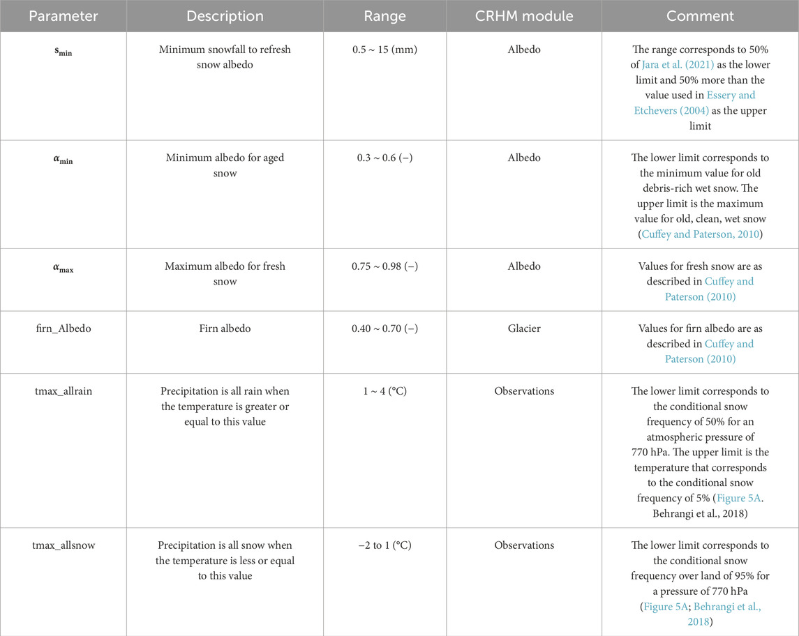
Table 2. Candidate parameters evaluated in DELSA with their respective ranges for calibration.

We evaluated the model performance against albedo and surface elevation changes observed at the AWS, as reported by Kinnard et al. (2018) (Table 1). The evaluation follows a methodology similar to that shown by Pradhananga and Pomeroy (2022) and consists in calculating the difference in elevation and albedo using the mean bias error (MBE), root-mean-square error, and the Wang–Bovik index (WBI) (Wang and Bovik, 2002). The WBI serves to evaluate the similarities between observed and modeled variables based on the differences between means and variances (Pradhananga and Pomeroy, 2022). The WBI and its components are calculated using Equations 5-8 below:

$\mathbf{W}\mathbf{B}\mathbf{I}=\left[{\mathbf{m}}_{\mathbf{xy}}\right]*\left[{\mathbf{v}}_{\mathbf{xy}}\right]*\left[{\mathbf{R}}_{\mathbf{xy}}\right],(5)$

${\mathbf{m}}_{\mathbf{xy}}=\left[\frac{\mathbf{2}\left(\overline{\mathit{x}}-{\mathbf{\psi }}_{\mathbf{xy}}\right)*\left(\overline{\mathit{y}}-{\mathbf{\psi }}_{\mathbf{xy}}\right)}{{\left(\overline{\mathit{x}}-{\mathbf{\psi }}_{\mathbf{xy}}\right)}^{\mathbf{2}}+{\left(\overline{\mathit{y}}-{\mathbf{\psi }}_{\mathbf{xy}}\right)}^{\mathbf{2}}}\right],(6)$

${\mathbf{v}}_{\mathbf{xy}}=\left[\frac{\mathbf{2}*{\mathbf{\sigma }}_{\mathbf{x}}*{\mathbf{\sigma }}_{\mathbf{y}}}{{{\mathbf{\sigma }}_{\mathbf{x}}}^{\mathbf{2}}+{{\mathbf{\sigma }}_{\mathbf{y}}}^{\mathbf{2}}}\right],(7)$

${\mathbf{R}}_{\mathbf{xy}}=\left[\frac{\mathbf{2}*{\mathbf{\sigma }}_{\mathbf{xy}}}{{\mathbf{\sigma }}_{\mathbf{x}}*{\mathbf{\sigma }}_{\mathbf{y}}}\right],(8)$

where ${\mathrm{\psi }}_{\text{xy}}$ are the minimum values between the observed and simulated ${\mathrm{x}}_{\mathrm{i}}$ and ${\mathrm{y}}_{\mathrm{i}}$, respectively; $\overline{x}$ and $\overline{y}$ are the means; ${\mathrm{\sigma }}_{\mathrm{x}}$ and ${\mathrm{\sigma }}_{\mathrm{y}}$ are the standard deviations; and ${\mathrm{\sigma }}_{\text{xy}}$ is the covariance. In addition, ${\mathrm{m}}_{\text{xy}}$ is the difference in means, ${\mathrm{v}}_{\text{xy}}$ is the difference in variances, and ${\mathrm{R}}_{\text{xy}}$ is the Pearson correlation coefficient.

Time variability of hydroglaciological variables

We identified change points in various glaciological variables of interest, including mass balance, runoff, and equilibrium altitudinal line based on that presented by Fealy and Sweeney (2005). We visually identified points in time where glaciohydrological variables displayed trends by computing the cumulative sum of deviations (CUSUMs) from the historical mean. Additionally, we employed Pettitt’s nonparametric test (Pettitt, 1979) to confirm these change points. The equation used to perform the CUSUM analysis is shown in Equation 9:

${\mathbf{S}}_{\mathbf{i}}={\displaystyle \sum _{\mathit{i}=\mathit{n}}}\left({\mathbf{x}}_{\mathbf{i}}-\mathbf{k}\right),(9)$

where S_i is the CUSUM metric, ${\mathbf{x}}_{\mathbf{i}}$ represents the yearly value of the variable of interest, and k is the average of the historical series of $\mathrm{x}$. Furthermore, we employed the Mann–Kendall test to determine the statistical significance of the trends observed in the annual time series.

Results

Parameter sensitivity and calibration

Figure 4 illustrates the DELSA first-order sensitivity analysis applied to the uncalibrated CRHM model of the Universidad Glacier. Of the three most sensitive parameters, ${\mathrm{\alpha }}_{\min }$ represents the lower limit of snow albedo and ${\mathrm{S}}_{\min }$ is the minimum snowfall required to update snow albedo to its maximum value. In contrast, tmax_allsnow controls the simulated precipitation partition in solid and liquid phases. These three parameters were selected for the calibration.

Figure 4

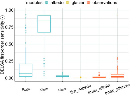
Figure 4. DELSA first-order sensitivity of the selected CRHM parameters. DELSA was conducted with a sample size of n = 100. The y-axis indicates the first-order sensitivity of each parameter. The sum of the sensitivities of the six parameters in each iteration is equal to 1, with the parameter having the highest first-order value exerting the greatest influence on the variables analyzed. In this case, the parameter that has the greatest impact on the mass balance is α_min.

The calibrated parameter values are presented in Table 3. Both calibrated models exhibit similar values for ${\mathrm{\alpha }}_{\min }$, indicating convergence of this parameter. The main difference between the models lies in the value of parameter ${\mathrm{S}}_{\min }$. A lower value of S_min indicates that a smaller amount of snow is required to completely refresh the snow albedo, which results in the snow surface absorbing less solar energy overall as the albedo is refreshed more frequently. A similar effect results from the calibrated value of ${\mathrm{\alpha }}_{\min }$ compared with the default parameter value. The calibration process reduced the mass balance error by more than three times when comparing the model calibrated with the extended period (crec) to the uncalibrated model (unc), as shown by the RMSE values in Table 3.

Table 3

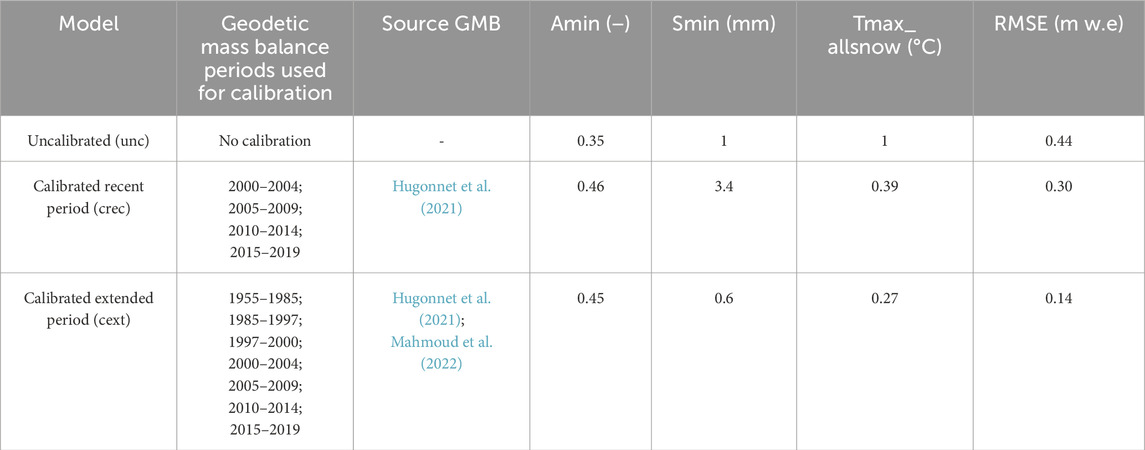
Table 3. Calibrated models, along with their corresponding parameter values and sources of calibration. The “uncalibrated” (unc) model represents the model with all parameters obtained, as described in the Methodology section. The “calibrated recent period” (crec) model is calibrated using elevation differences obtained from Hugonnet et al. (2021), which were converted into mass balances considering an ice density of 850 kg/m³ and the glacier outlines of 2018. The “calibrated extended period” (cext) model is calibrated using data from Hugonnet et al. (2021) and mass balances for the years 1955–1997 from Mahmoud et al. (2022). The RMSE values shown correspond to those calculated using all available mass balances, i.e., between 1955 and 2020. For the crec case, which was calibrated against the GMB during the 2000 period, the RMSE value for the calibration was 0.07 m w.eq.

Model evaluation

In this section, we compare the simulated daily mean albedo and surface height change with observations at the AWS, as shown in Figure 1. The results of various evaluation metrics for albedo and surface height changes are provided in Supplementary Tables S1 and S2, respectively.

Figure 5 displays the time series of the three AWS observation sites. AWS L. Z. (Figures 5A–C) was located in the ablation zone and has the longest record covering both accumulation and ablation seasons for the year 2013/14. AWS E.U.Z. (Figures 5D–F) was located in the eastern accumulation zone during the 2012/13 season and then relocated to the western accumulation zone for the next season. Hence, here it is called AWS W.U.Z. (Figures 5G–I). For AWS L.Z., all three models perform well in terms of albedo (Figure 5B; WBI >0.87, RMSE <0.15, and MBE <0.05) and surface height changes (Figure 5C; WBI >0.95, Percent Bias <18%, and MBE <0.12). The models successfully capture the albedo variability and surface elevation height during the accumulation period, with Pearson correlation values exceeding 0.97. However, their performance decreases during the ablation period. The simulated albedo experiences a rapid decay at the beginning of October, leading to swift snowmelt. This accelerated decay in the snowpack mass is halted by snowfall at the beginning of November, which is not sufficient to increase accumulation but refreshes the albedo and thus delays the complete disappearance of the snowpack. Despite the overestimation of albedo in the ablation season and an accelerated decay in the accumulation season, the maximum accumulation differs by less than 40 cm in surface elevation, and there is only a 1-week difference in the total disappearance of the snowpack with respect to the observed conditions.

Figure 5

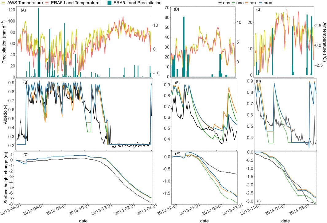
Figure 5. Point-scale CRHM simulation results. Panels (A–C) show meteorology, albedo, and surface height elevation change, respectively, in the ablation zone AWS (AWS L.Z.); panels (D–F) show meteorology, albedo, and surface height elevation change, respectively, in the easternmost accumulation zone (AWS E.U.Z.); panels (G–I) show meteorology, albedo, and surface height elevation changes, respectively, in the westernmost accumulation zone (AWS W.U.Z.).

For the 2012/2013 ablation season at AWS E.U.Z, the calibrated models demonstrate favorable performance in albedo simulation (Figure 5E), maintaining high values of temporal (r-Pearson >0.81) and variability (Vxy >0.92) correlations. The calibrated models show a slight positive bias in snow albedo, whereas the default parameters result in albedo values that generally underestimate measurements. Simulated surface elevation changes correlate well with measurements (Figure 5F; r-Pearson >0.98), indicating a period of stability until the first week of January, followed by a rapid decline during a period of increased temperature, with a smoother decline in February. The fact that the worst performing metric in the WBI is the difference in variance (Vxy <0.77), along with high percent bias values (percent bias (PBIAS) >92%, Supplementary Table S1) shows that all models tend to overestimate the ablation of the snowpack and glacial ice at this location. The best results are obtained when comparing the simulated values with the observations from the western portion of the accumulation zone (AWS W.L.Z.). PBIAS values in all cases are less than 16%, with a very low value of −0.4% for the uncalibrated model. It is important to consider that the AWS records correspond to site measurements, are highly sensitive to local topography, and may not necessarily be representative of the average behavior of the HRU in which the model is discretized.

The simulated mass balance at the glacier scale for the hydrological year 2012/13 is shown in Supplementary Table S2 and illustrated in Figure 6. Supplementary Table S3 provides the values of the annual (MBA), summer (MBS), and winter (MBW) mass balances for the different calibration scenarios, along with the results from glaciological (stake) measurements conducted by Kinnard et al. (2018). In Figure 6, mass balance at the ablation stakes installed by Kinnard et al. (2018) is compared to the simulated results at the HRUs overlapping with these stakes. At the ablation stakes, the three models generally represent the winter mass balance well in 2012, although they underestimate accumulation values below 3,100 m a.s.l. However, since the glacier area below this elevation accounts for only 12% of the total glacier, this discrepancy has minimal impact at the overall glacier scale. Difficulties arise in replicating the steep mass balance gradient observed in the summer of 2012/13, with an overestimation of ablation at higher elevations (3,400–4,000 m a.s.l.) and underestimation below 2,800 m a.s.l. For the hydrological year 2013/14, all three models experience a decrease in performance, underestimating winter accumulation and summer ablation. In the glaciological mass balance, both years exhibit similar winter mass balances of 1.43 m w. e. (2012) and 1.48 m w. e. (2013). Capturing this similarity is challenging for the models because of the 27% lower winter precipitation in 2013 than in 2012, according to the meteorological input product. Discrepancies in the gradients depicted in Figure 6 for the winter balance in 2013/14 primarily occur above 3,600 m a.s.l. The underestimation of the winter balance could be attributed to phenomena that are not explicitly represented in our model, such as the occurrence of wind-transported snow from adjacent basins or shading effects within each HRU. Further improvements of the model could, for instance, add snow source areas upwind of the glacier boundaries that may explain local high accumulation effects and investigate preferential deposition effects with higher-resolution numerical weather predictions. Despite the above, at the glacier scale, both calibrated models demonstrate good agreement with the glaciological mass balance reported by Kinnard et al. (2018). For the annual mass balance, differences are less than −0.25 m w.e. for the hydrological year 2012/13 and less than 0.43 m w.e. for 2013/14. These differences fall within the uncertainty range of glaciological mass balances.

Figure 6

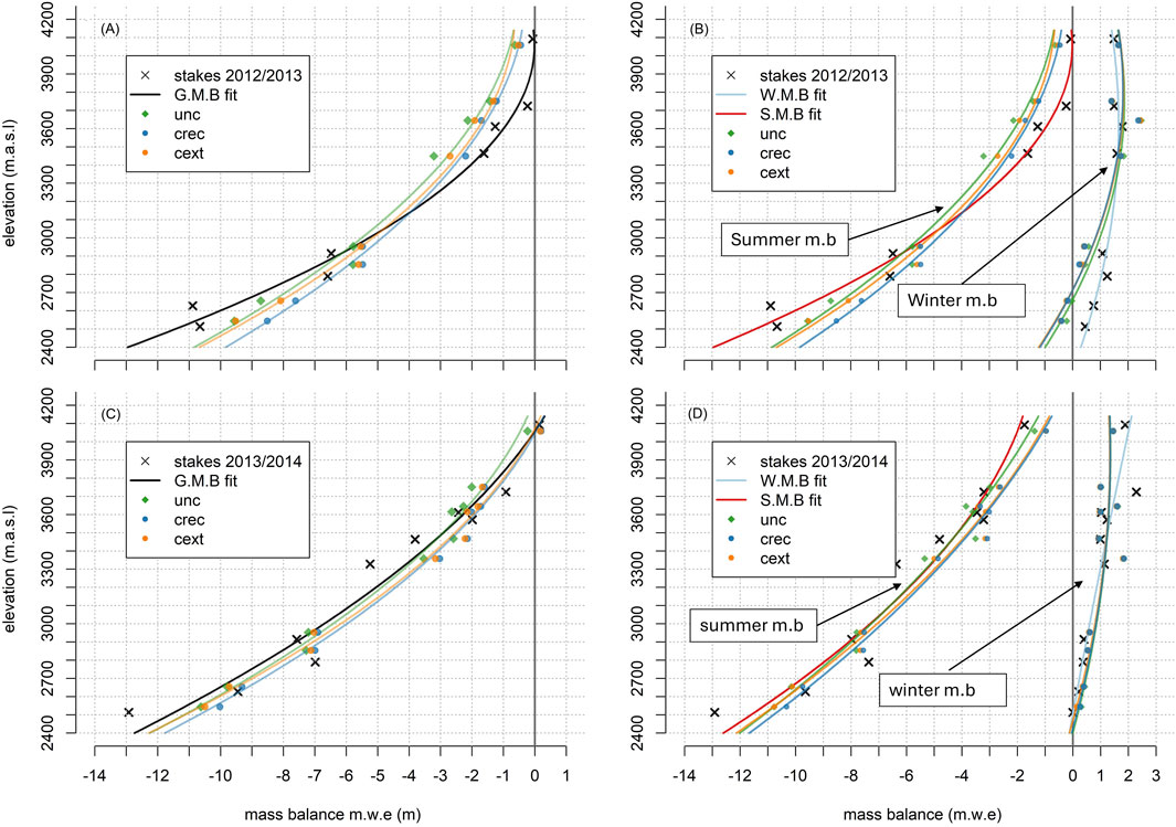
Figure 6. Measured and modeled mass balances at ablation stake locations. Black crosses represent the ablation stakes installed by Kinnard et al. (2018). The dots represent the mean elevation and mass balance of the HRU overlapping the stake location. Continuous lines show a second-order polynomial fit curve; for dots and lines, the color indicates which model they correspond to, and the black line shows the best-fit line to the observations. (A) Annual mass balance for the glaciological year 2012; (B) seasonal mass balance for the glaciological year 2012; (C) annual mass balance for the glaciological year 2013; and (D) seasonal mass balance for the glaciological year 2013.

Mass balance time series for the historical period

Figure 7 presents the simulated mass balance for the different models alongside the results of the CUSUM analysis. This visualization allows for a clear comparison of mass balance trends and cumulative effects over time across various model configurations. Mass balance CUSUM analysis identified two statistically significant change points. The first occurred in 1971 and marked the end of a period characterized by sustained glacier mass loss from 1955 to 1971, where only four years experienced a positive or near-equilibrium mass balance (Figure 7A). This period is evident in the continued CUSUM decay (Figure 7B). The models show high ablation rates during this period, with −2.53 m.w.e. per year for the cext model.

Figure 7

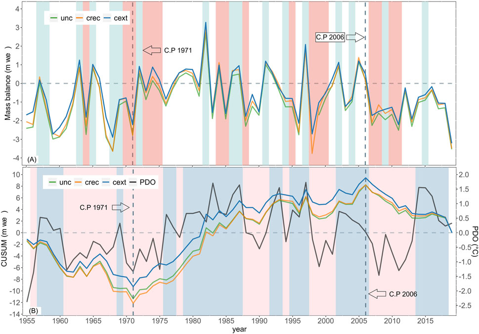
Figure 7. (A) Time series of simulated annual mass balances. Niña years (ONI < −0.5) are highlighted in red stripes, whereas the light blue stripes correspond to Niño years (ONI > 0.5). (B) CUSUM analysis for annual mass balance and PDO index. The gray dotted line corresponds to the statistically significant change points found through CUSUM and verified with Pettitt’s test (p-values <0.04). Blue stripes indicate positive phases of PDO (>0), and red stripes indicate negative phases (PDO < 0).

Between 1971 and 2006, we obtained a period of near-equilibrium mass balance for the Universidad Glacier, with the cext model estimating a value of −0.07 m w.e. In the early years of this period (1972–1982), the models estimate a positive mass balance, with almost all years having positive or neutral values [0.54 (cext), 0.35 (crec), and 0.05 (unc) m w.e.]. This period is followed by a period of slightly negative cumulative mass balance between 1982 and 2006, with all models calculating average negative mass balances (cext −0.22, crec −0.34, and unc −0.64 m w.e.). Despite the different behaviors of these two subperiods, we did not identify statistically significant change points within this time window. The annual mass balance exhibits a moderate temporal correlation with ENSO, with an r-Spearman of 0.41. It is also noteworthy that, of the 18 years in which all the models calculated a positive mass balance, nine correspond to El Niño years, two to La Niña years, and seven to neutral years. The highest simulated mass balance (cext model) occurred in 1982 (3.27 m w.e.) and 1997 (2.09 m w.e), which are very strong El Niño years. The other very strong El Niño year in the simulated period is 2015, but this year did not show a similar mass balance behavior. All the strong El Niño years occur before the year 2000, and they show an annual mass balance of approximately 1.0 m w.e. (more details in Supplementary Table S4).

The CUSUM analysis and, consequently, the identified change points show a relationship with the predominant phases of the Pacific Decadal Oscillation (PDO). Although the correlation between the PDO and the CUSUM statistic for the entire period is weak, with an r-Spearman of 0.32, this relationship is stronger in the 1955–2006 period, with an r-Spearman of 0.52. The first period (1955–1971) is mainly dominated by negative PDO anomalies, with a negative PDO phase occurring from 1960 to 1974. Although the CUSUM point of change in 1971 does not coincide directly with a PDO phase change, a clear positive trend is observed (p-values MK test <0.01) that clearly coincides with the CUSUM statistic, both starting in 1971 and ending in 1986. The second period, delimitated between the change points in 1971 and 2006, is mainly characterized by a positive PDO phase that began in 1976 and ended near 2006 (Boisier et al., 2016). From the second point of CUSUM change, the relationship between mass balance and ENSO and PDO indices is lost, as can be seen in the decay of Spearman’s correlation.

Figure 8 illustrates the cumulative mass balance for the Universidad Glacier, derived from geodetic mass balances and modeled using different calibration scenarios. Additionally, the cumulative mass balance of the Echaurren Norte Glacier, situated approximately 126 km north of the Universidad Glacier and serving as the reference glacier of the World Glacier Monitoring Service, is depicted in panel 8 (B). The vertical dashed lines in 1971 and 2006 show the change points found by CUSUM analysis (Figure 7B). The second change point in 2006 marks a period of sustained mass loss, characterized by the lowest annual mass balance, primarily driven by the lowest estimated winter mass balance. Additionally, this period exhibits the lowest interannual variability. Since 2007, no year has shown a positive mass balance, with only 2012 and 2016 being close to equilibrium.

Figure 8

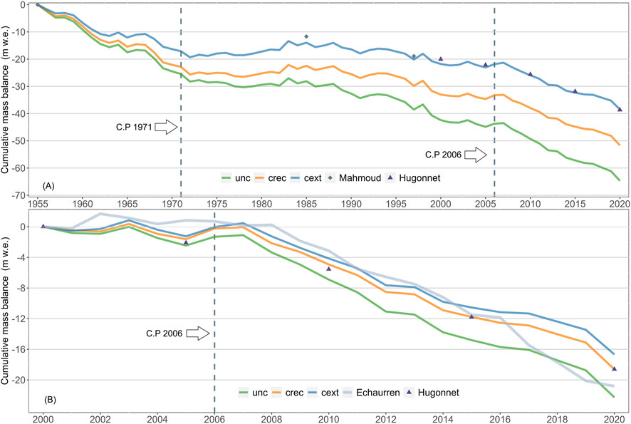
Figure 8. (A) Time series of cumulative mass balances simulated by different CRHM models. Gray diamonds and purple triangles correspond to the cumulative mass balances calculated from geodetic mass balances from Mahmoud et al. (2022) and Hugonnet et al. (2021), respectively. (B) Time series of cumulative mass balance from different CRHM models since 2000. The gray line corresponds to the cumulative mass balance of the Echaurren Norte Glacier.

As expected, given the different calibration objectives, the cext model exhibited better performance in simulating the accumulated mass balance for the entire study period. The crec and unc models overestimate end-of-period glacier losses by approximately 10 m w.e. (25%) and 25 m w.e. (63%), respectively. For the period 2000–2020, characterized by significant glacier losses, the crec model performed better. Relative to the best-performing simulation, cext model underestimated glacier losses by 2 m w.e. (11%), whereas the unc model overestimated ice mass loss by 8 m w.e. (44%). The difference between the models is explained almost entirely by the differences in summer mass balance. Whereas the percent bias between the models is equal to or less than 2% for the winter mass balance, the difference between the unc and cext models is −18% for the summer mass balance. However, it is −8% between the cext and crec simulations (Supplementary Table S3).

Equilibrium-line altitude

Figure 9 illustrates the evolution of the equilibrium-line altitude (ELA) for the different study cases, accompanied by the CUSUM analysis to identify the change points. The cext model consistently exhibits the lowest ELA, aligning with its higher annual mass balance. On average, the difference between the cext and unc models is 31 m, and that between the unc and crec models is 20 m (Supplementary Table S3).

Figure 9

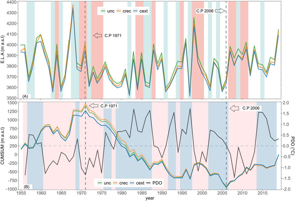
Figure 9. (A) Simulated ELA time series. Niña years are highlighted in red stripes, and light blue stripes correspond to Niño years. (B) CUSUM analysis of annual mass balance and PDO index. The dark gray dashed line corresponds to the statistically significant change point found through CUSUM and verified with Pettitt’s test (p-values <0.04). The light gray dashed line represents the neutral PDO phase.

Considering that the ELA falls between 3,630 and 3,960 m a.s.l. in 50% of the years, the percentage difference in terms of area change in the accumulation area ratio (AAR) is approximately 3% of the glacier for every 30 m elevation. In other words, there is approximately 3% less accumulation area in the unc model compared to the cext and 2% less accumulation area in the crec compared to the cext model. As for the mass balance and glacier discharge, the three models exhibit the same change points and trends.

In the ELA CUSUM analysis, we identified the same change points in 1971 and 2006 as in the mass balance case. The period between 1955 and 1971 is characterized by high interannual variability and no clear trend. The second period between 1971 and 2006 exhibits a lower average ELA, whereas the period from 2006 to 2019 shows a higher average ELA and lower variability. Since 1971, we found a statistically significant trend of +35 m per decade (increased elevation).

In Supplementary Table S3, the comparison between the simulated ELA and the glaciological mass balance for the years 2012/13 and 2013/14 shows an overestimation of the ELA by approximately 200 m for the year with the highest mass balance (2012/13) and an underestimation by approximately the same value for the year with the lowest mass balance (2013/14).

Glacier runoff

Figure 10A illustrates the annual average glacier discharge from the Universidad Glacier for the three calibration scenarios. Glacier discharge is computed as the sum of simulated firn, ice, and snow melt. Figure 10B presents the CUSUM analysis of the annual average glacier discharge alongside the PDO anomalies. The difference between the models exhibits a similar pattern as in the mass balance, showing a bias but comparable interannual variability. This is evident from the standard deviation of the simulated series (Supplementary Table S5). The percentage bias between the cext model, considered as a reference, and unc and crec models remains consistent throughout the study period. The unc model, characterized by more negative mass balances, yields a higher water contribution, overestimating glacier runoff by 24% compared to the cext model. In contrast, the crec model shows a slightly lower overestimation of approximately 7%. These differences increase when analyzing the summer runoff, with a 25% difference between the unc and cext models and an 11% difference between the crec and cext models.

Figure 10

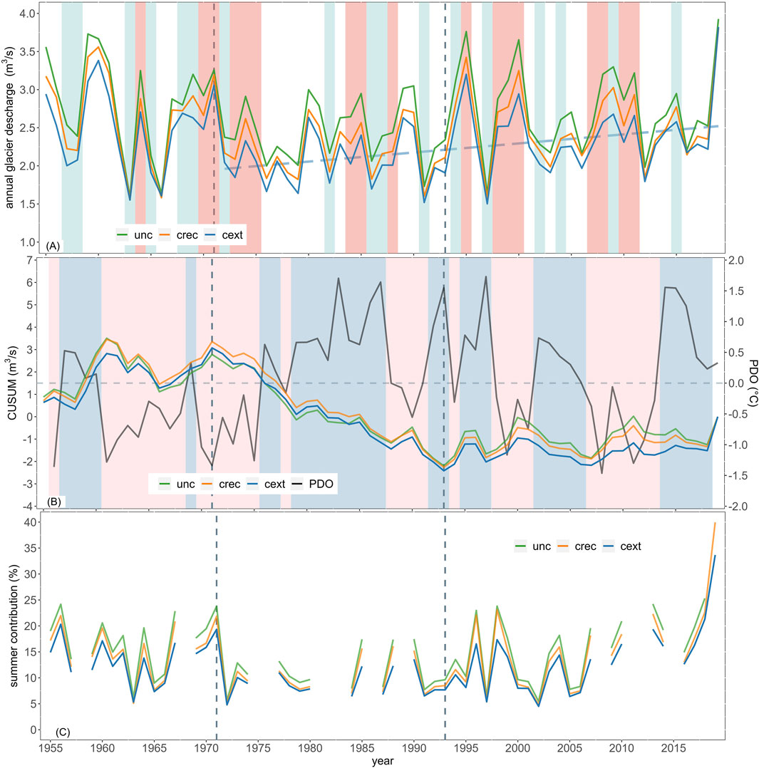
Figure 10. (A) Average annual glacier discharge for the three models. Light blue stripes indicate a Niño year, whereas the red stripes indicate a Niña year. The dashed blue line from 1971 to 2019 indicates a statistically significant increasing trend. (B) CUSUM analysis of annual glacier discharge together with the PDO anomaly. The blue and red stripes indicate the positive and negative phases of the PDO, respectively. (C) Relative contribution of the Universidad Glacier ice melts to the entire Tinguiririca Bajo Los Briones Basin (Figure 1C) for the JFM months.

Due to this almost identical behavior in the year-to-year variations of the models, the analysis of change points and trends yields consistent results. In the CUSUM analysis, two statistically significant change points were identified: 1971 and 1993 (p-value <0.07). The first period between 1955 and 1971 is characterized by the highest mean and interannual variability during the study period. The change point is the same as that in the mass balance and emerges clearly in the CUSUM analysis. Between 1971 and 1993, there is a period of relatively low glacier discharge owing to the neutral mass balance between 1972 and 1982. The second change point in 1993 is attributed to the occurrence of four La Niña events between 1995 and 2000, leading to a decrease in precipitation compared to the period after 1971. This results in a significant increase in the magnitude of ice and firn melt between 1995 and 2000, as evidenced by the change in slope in the CUSUM during those years. In 2006, there is also a change in slope, coincident with the change point for the mass balance, but this change is not statistically significant according to the Pettitt test. From the first change point in 1971, there is an increasing trend in glacier discharge of 0.18 m³/s per decade for all the models (significant after the Mann–Kendall test <0.05).

There is an inverse moderate correlation between ENSO and glacier discharge, with a Spearman correlation of −0.46. The relationship between the CUSUM index and PDO is −0.35, indicating a weak correlation at the decadal time scale. Similar to the mass balance, the relationship between discharge and ENSO and between discharge and PDO is stronger before 2010. Consider the period until the second change point (1955–1993) when the correlation between the PDO and the CUSUM is −0.6. Even if we consider the period between 1955 and 2006, the correlation is −0.51. In the case of ENSO, for the period before the second change point, the correlation is maintained, but when considering the period between 1955 and 2006, the correlation increases to −0.55.

Figure 10C shows the relative summer (JFM) contribution of glacier (snow, firm, and ice) melt to the river flow at the Tinguiririca Bajo Los Briones (TBLB) stream gage. Trimesters with less than 80 days of data are not shown. Three distinct periods were identified, which are coincident with the change points illustrated in panels (A) and (B). First, before 1971, the summer contribution ranges between 5% and 25%, with an approximate mean of 15%. Then between 1971 and 1993 (the wetter period), summer contributions decrease in magnitude and variability. After 1993, variability increases, and the magnitude initiates a visible upward trend around 2003. Water years after 2010 (the so-called Chile megadrought) see summer contributions from the glacier in the order of 15%–35% to the larger basin flow.

Discussion

Parameter sensitivity and calibration

Successful calibration of the cext model, emphasizing a reduced number of highly sensitive parameters within a physically reasonable range, demonstrates that a physically based energy-balance model can effectively represent the mass balance in a long-term simulation. Snow albedo parameters are relevant in this context, as snow isolates the glacier ice from the atmosphere, thus shielding it from shortwave radiation (Munro and Young, 1982). This suggests the potential application of similar modeling approaches for extended periods. In addition, mass balance interannual variability exhibits striking similarities between the calibrated models (cext and crec) and the model without calibration, enabling the identification of trends and periods across the models. This highlights the influence of the forcing data, which is expected, but also suggests that a physically based model without calibration, with a judicious selection of parameters, holds significant utility for studying the annual behavior of glacier variables such as mass balance or runoff. The models (uncalibrated and calibrated) yield a slightly higher overall albedo than the observations at the AWS. The surface elevation changes, however, are by and large correctly simulated at two of the three AWS locations, namely, for the AWS L.Z. (glacier tongue) and AWS W.U.Z., whereas at AWS E.U.Z., the ablation rate is quite higher than that observed (Figure 5). At the ablation stakes, the model behavior is such that mass balance at the upper elevation is overestimated (more mass loss than observed), whereas mass balance at the tongue is underestimated (less mass loss than observed). In all cases, the first difficulty lies in comparing point-scale observations with estimates at the HRU scale. The specific location of each AWS in relation to the average physiography of the HRU may introduce biases in both the accumulation and solar radiation, which may override the higher albedo effect. This may affect AWS E.U.Z., as it lies near the boundary between two HRUs with different sun exposures.

The largest differences in the simulated results emerge when calculating the cumulative mass balance, as ablation rates are different between models. Although the differences vary from period to period, the uncalibrated (unc) and cext models always present the highest and lowest ablation rates, respectively. This difference propagates in time and causes the cumulative mass balance to differ considerably at the end of the simulated period among models. As an example, based on radio-echo sounding data, the total volume of glaciers was estimated to be 1.63 km³ w.e. in 2012 (DGA, 2012). Assuming the same area as in 2010 and using the calculated GMB, we estimated a volume of 2.49 km³ w.e. in 1955. Calculating the volume loss with the different models, starting from the 2.49 km³ w.e. in 1955, the unc model indicates a volume loss of 72%, the crec model indicates a loss of 54%, and the cext model indicates a loss of 44%. The time difference in arriving at the same ice loss between the calibrated (cext) and uncalibrated (unc) models is approximately two decades, which is a relevant time scale for the evaluation of adaptation strategies to climate change in the water resource arena. This suggests that for climate change projections, parsimonious glaciological parameter adjustment within plausible ranges against long-term geodetic mass balance estimates is granted and could constrain model parameter uncertainty.

Universidad Glacier mass balance evolution

The time periods and evolution of the Universidad Glacier estimated in this study are consistent with the results of different glacier studies in the central Andes. Our results align well with those of Masiokas et al. (2016), who simulated the Echaurren Norte Glacier mass balance and verified a period of sustained loss from the 1940s to the early 1970s. This fact is also represented by the correlation between ENSO and the mass balance of the Echaurren Norte Glacier (Farías-Barahona et al., 2019). In contrast, Ayala et al. (2020), in their modeling of the Maipo Basin (33° to 34°), found a nearly neutral period between 1955 and 1968, followed by a more negative mass balance between 1968 and 1975. The difference between our study and Ayala et al. (2020) for the period 1955–1968 could be attributed to climatic differences in the study areas or the lower elevation of Universidad Glacier compared to the average elevation of the glaciers modeled by Ayala et al. (2020) (3,800 m a.s.l) for their southernmost subbasin, which is closest to the Universidad Glacier. Additionally, the 1955 DEM used in this work differs in its processing scheme from that of Ayala et al. (2020), resulting in a product with a significantly higher resolution. Our findings also align well with the evolution of the Guanaco Glacier, a high-altitude glacier (>5,000 m a.s.l.) located in the Desert Andes (29.34°S, 70.01°W), where the mass balance reconstructed from precipitation and vapor pressure deficits, along with streamflow-based reconstructions, shows a period of predominantly negative mass balance (1935–1975), followed by a period of alternating negative and positive mass balances (1975–2005), and a highly negative mass balance from 2005 to 2015 (Kinnard et al., 2020).

Wilson et al. (2016) investigated fluctuations in glacier area and surface ice velocity of the Universidad Glacier between 1967 and 2015 using different satellite images. They recorded a retreat of 177 m in the Universidad Glacier between 1969 and 1985, along with an increase in glacier surface velocity in 1985 compared to 1969. Between 1971 and 2006, there were two brief periods of equilibrium, 1991–1993 and 2001–2006, observed as an upward slope in the CUSUM analysis (Figure 9). These periods were correlated with a slight increase in ice surface velocity and glacier front advances (Wilson et al., 2016). Wilson et al. (2016) postulated that the observed increases in ice velocity could be due to periods of positive mass balance experienced by the Universidad Glacier due to the relationship between mass balance and ice velocity. However, the presence of a surge registered by Lliboutry (1958) in 1943 hinders this hypothesis, as the velocity increases could be attributed to surge cycles specific to the glacier. The agreement between our findings and those of Wilson et al. (2016) underscores the underexplored potential of estimating mass balance through its relationship with changes in ice surface velocity obtained from historical optical imagery in combination with numerical simulations.

Because the developed model does not adjust the glacier geometry owing to mass loss or gain, it can be categorized as a reference surface balance (Elsberg et al., 2001). This type of mass balance may underestimate mass loss when using the glacier geometry at the end of the simulation period, as is the case of our model, or overestimate mass loss when using the initial glacier geometry (Huss et al., 2010). Although calibrated models may underestimate mass loss, Huss et al. (2010) observed that the interannual variability and trends in mass balance did not differ significantly when comparing a fixed geometry model with a geometry-adjusted model. They noted that the largest long-term differences depended strongly on the retreat of the glacier, with the glaciers whose tongues had steeper slopes showing the largest discrepancies. Similarly, Kinnard et al. (2022) observed a relatively small difference of 5.6% between a conventional mass balance simulation and a reference cumulative balance with a fixed area of 1976 for a valley glacier. This small difference is attributed to the glacier’s retreat being mainly constrained to the lower part of the valley, within a limited elevation range. In the case of Universidad Glacier, we observed that the glacier terminus has a gentle slope (Figure 2). This is also supported by the fact that the Universidad Glacier has experienced a moderate retreat compared to other glaciers in the semi-arid Andes, with only 6% of their area reduced between 1945 and 2011. For instance, the Juncal Sur, Olivares Alfa, Olivares Beta, and Olivares Gamma glaciers with steeper slopes in their termination zones have lost 34%, 32%, and 20%, respectively (DGA, 2011). This suggests that in our case study, the uncertainty driven by glacier geometry is minor compared with other factors.

Runoff and ELA

Our findings reveal notable interannual variability in glacier discharge and its contribution to the lowlands downstream (“Tinguiririca Bajo Los Briones” streamflow gage), particularly during the summer months, with values ranging from 3% to 34%. In the summer of 2009/2010, Bravo et al. (2017) estimated a contribution of 10%–13% from the Universidad Glacier, considering both ice and snow melt. For the same period, the cext model, which calculates the lower contribution, estimates 12%, considering ice, firn, and snow melt. Since the area used by Bravo et al. (2017) is 29 km², corresponding to the limits of the glacier in 2000, which is 11% larger than the area recorded in 2020 used in this study, our estimates of ablation are slightly larger than those estimated by Bravo et al. (2017). These differences can be attributed to the variations in the modeling approach used. Bravo et al. (2017) used a distributed degree-hour model calibrated at a site scale and forced with local meteorology from an AWS, whereas we used an energy balance model forced with reanalysis products. Additionally, Bravo et al. (2017) did not estimate the effects of debris cover on the glacier tongue, which can accelerate the ablation process (Rounce et al., 2021).

Ayala et al. (2020) also found strong interannual variability in the glacier contribution for the Maipo Basin, estimating that the ice melt can vary from less than 10% to more than 90%, as in the year 1968/1969. For the years 1968/1969, we calculated the fourth highest glacier discharge; however, due to the lack of streamflow data for those years, it is not possible to calculate the percentage of summer contribution. In terms of magnitude, for the period 1955–2015, Ayala et al. (2020) estimated an ice melt runoff equal to 596 mm yr⁻¹ for the Maipo glaciers. This is considerably lower than our estimate of 1,635 mm yr⁻¹ for the same period and is consistent with the different climatology of the Universidad Glacier, located in a region with over 2,000 mm yr⁻¹ of annual precipitation (González-Reyes et al., 2017). The increasing trend in glacier discharge observed between 1971 and 2019 aligns with the projections of Escanilla-Minchel et al. (2020). Using a degree-day model, they projected changes in glacier runoff for the period 2020–2100, with a reference period of 2008–2014. Their findings indicate that the Universidad Glacier will experience an increase in runoff under RCP 4.5 and RCP 8.5 scenarios until around 2040, followed by a gradual decline in glacier runoff. This suggests that the “peak water” period for this glacier has not yet been reached.

Our results indicate an increase of 35 m per decade in the ELA of the Universidad Glacier since 1971, resulting in an approximately 8% reduction in the accumulation area. Ayala et al. (2020) also observed a positive trend in ELA elevation for the Maipo glaciers, with an increase of 39 m per decade between 1955 and 2015. Barria et al. (2019), using a relationship between the 0-degree isotherm altitude (ZIA) and precipitation, derived an estimate of the ELA at a regional scale (between 33 and 34S). They found a statistically significant trend in the ELA elevation of 64 ± 8 m per decade for the period 1978–2018. Additionally, Barria et al. (2019), through CUSUM analysis, identified an abrupt change in the ZIA in 1976, close to our change point in 1971. Despite differences in the magnitude of the trend and change points with Barria et al. (2019) and Ayala et al. (2020), our results are consistent, revealing the presence of an increasing trend in ELA since at least the mid-1970s.

Conclusion

The CRHM-glacier model was used to explore the interannual variability of the Universidad Glacier mass balance, with a limited calibration exercise to evaluate the potential of extended-period geodetic mass balance estimates to inform model development. The calibration process using geodetic mass balance estimates allowed for the adjustment of a small number of physically plausible parameters, leading to an improvement in model performance. At the site scale, no model shows a clear superiority compared to the in situ records of albedo and snowpack height. Although all three models accurately represent the measurements at the automatic meteorological station located in the ablation zone between 2012 and 2014, they face greater difficulties in reproducing the variables recorded by the stations located in the accumulation zone. Calibration of albedo parameters resulted in reduced ablation, and the total albedo of the glacier on a daily scale exhibited an enhanced performance. Although the annual scale differences between the models are small, their cumulative effects become significant over the long term. This is particularly crucial for glacier mass projections in climate change studies.

The mass balance of the Universidad Glacier exhibited a moderate correlation with the PDO. The positive phases of the PDO coincide with periods of slightly positive or neutral mass balance, whereas the negative phases align with pronounced periods of mass loss. Additionally, the ENSO phenomenon demonstrates a moderate relationship with annual mass balance, where strong to very strong Niño events correspond to larger winter accumulation. However, since the initiation of the Chile megadrought in 2010, this relationship has been interrupted. When projecting glacier evolution under climate change scenarios for water resource planning objectives, these modes of interannual variability should be given appropriate attention, as they can result in decades of delay or acceleration in ice mass evolution. The sharp decrease in glacier MB detected since approximately 2006 can be explained primarily by a decrease in winter MB (precipitation effect). Nevertheless, we identify an apparent upward trend in glacier melt (summer MB) since the beginning of the 21st century. The linkages between precipitation and glacier albedo decay merit further research if reliable projections of glacier evolution and ice melt runoff can be obtained in future climates.

Data availability statement

The raw data supporting the conclusions of this article will be made available by the authors without undue reservation.

Author contributions

AM: investigation, writing–original draft, and data curation. JM: conceptualization, supervision, writing–review and editing, and validation. HM: data curation, resources, and writing–review and editing. DF-B: data curation, methodology, and writing–review and editing. CK: data curation, writing–review and editing, and formal analysis. ShM: data curation, validation, writing–review and editing, and formal analysis. SaM: formal analysis, validation, and writing–review and editing. MS: writing–review and editing and validation. AF: formal analysis, writing–review and editing, funding acquisition, and project administration.

Funding

The author(s) declare that financial support was received for the research, authorship, and/or publication of this article. AM was partially supported by project FONDECYT 1201429 and grant ANID-Magister Nacional 2021 folio 22211060.

Conflict of interest

The authors declare that the research was conducted in the absence of any commercial or financial relationships that could be construed as a potential conflict of interest.

Generative AI statement

The author(s) declare that no Generative AI was used in the creation of this manuscript.

Publisher’s note

All claims expressed in this article are solely those of the authors and do not necessarily represent those of their affiliated organizations, or those of the publisher, the editors and the reviewers. Any product that may be evaluated in this article, or claim that may be made by its manufacturer, is not guaranteed or endorsed by the publisher.

Supplementary material

The Supplementary Material for this article can be found online at: https://www.frontiersin.org/articles/10.3389/feart.2025.1517081/full#supplementary-material

References

Annandale, J., Jovanovic, N., Benad, N., and Allen, R. (2002). Software for missing data error analysis of Penman-Monteith reference evapotranspiration. Irrigation Sci. 21, 57–67. doi:10.1007/s002710100047

CrossRef Full Text | Google Scholar

Aubry-Wake, C., and Pomeroy, J. W. (2023). Predicting cydrological change in an alpine glacierized basin and its sensitivity to landscape evolution and meteorological forcings. Water Resour. Res. 59, e2022WR033363. doi:10.1029/2022WR033363

CrossRef Full Text | Google Scholar

Aubry-Wake, C., Pradhananga, D., and Pomeroy, J. W. (2022). Hydrological process controls on streamflow variability in a glacierized headwater basin. Hydrol. Process. 36 (10), e14731. doi:10.1002/hyp.14731

CrossRef Full Text | Google Scholar

Ayala, A., Farías-Barahona, D., Huss, M., Pellicciotti, F., McPhee, J., and Farinotti, D. (2020). Glacier runoff variations since 1955 in the Maipo river basin, in the semiarid Andes of central Chile. Cryosphere 14, 2005–2027. doi:10.5194/tc-14-2005-2020

CrossRef Full Text | Google Scholar

Barandun, M., Bravo, C., Grobety, B., Jenk, T., Fang, L., Naegeli, K., et al. (2022). Anthropogenic influence on surface changes at the Olivares glaciers, central Chile. Sci. Total Environ. 833, 155068. doi:10.1016/j.scitotenv.2022.155068

PubMed Abstract | CrossRef Full Text | Google Scholar

Barcaza, G., Nussbaumer, S. U., Tapia, G., Valdés, J., García, J. L., Videla, Y., et al. (2017). Glacier inventory and recent glacier variations in the Andes of Chile, South America. Ann. Glaciol. 58, 166–180. doi:10.1017/aog.2017.28

CrossRef Full Text | Google Scholar

Barria, I., Carrasco, J., Casassa, G., and Barria, P. (2019). Simulation of long-term changes of the equilibrium line altitude in the central Chilean Andes Mountains derived from atmospheric variables during the 1958–2018 period. Front. Environ. Sci. 7, 2296–665X. doi:10.3389/fenvs.2019.00161

CrossRef Full Text | Google Scholar

Behrangi, A., Yin, X., Rajagopal, S., Stampoulis, D., and Ye, H. (2018). On distinguishing snowfall from rainfall using near-surface atmospheric information: comparative analysis, uncertainties and hydrologic importance. Q. J. R. Meteorological Soc. 144, 89–102. doi:10.1002/qj.3240

CrossRef Full Text | Google Scholar

Bernhardt, M., and Schulz, K. (2010). Snowslide: a simple routine for calculating gravitational snow transport. Geophys. Res. Lett. 37. doi:10.1029/2010GL043086

CrossRef Full Text | Google Scholar

Berthier, E., Floricioiu, D., Gardner, A. S., Gourmelen, N., Jakob, L., Paul, F., et al. (2023). Measuring glacier mass changes from space-a review. Rep. Prog. Phys. 86, 036801. doi:10.1088/1361-6633/acaf8e

CrossRef Full Text | Google Scholar

Boisier, J. P., Rondanelli, R., Garreaud, R. D., and Muñoz, F. (2016). Anthropogenic and natural contributions to the southeast Pacific precipitation decline and recent megadrought in central Chile. Geophys. Res. Lett. 43, 413–421. doi:10.1002/2015GL067265

CrossRef Full Text | Google Scholar

Braithwaite, R. J., and Hughes, P. D. (2020). Regional geography of glacier mass balance variability over seven decades, 1946–2015. Front. Earth Sci. 8, 2296–6463. doi:10.3389/feart.2020.00302

CrossRef Full Text | Google Scholar

Bravo, C., Loriaux, T., Rivera, A., and Brock, B. W. (2017). Assessing glacier melt contribution to streamflow at Universidad Glacier, central Andes of Chile. Hydrology Earth Syst. Sci. 21, 3249–3266. doi:10.5194/hess-21-3249-2017

CrossRef Full Text | Google Scholar

Burger, F., Brock, B., and Montecinos, A. (2018). Seasonal and elevational contrasts in temperature trends in central Chile between 1979 and 2015. Glob. Planet. Change 162, 136–147. doi:10.1016/j.gloplacha.2018.01.005

CrossRef Full Text | Google Scholar

Cannon, A. J. (2018). Multivariate quantile mapping bias correction: an n-dimensional probability density function transform for climate model simulations of multiple variables. Clim. Dyn. 50, 31–49. doi:10.1007/s00382-017-3580-6

CrossRef Full Text | Google Scholar

Compagno, L., Huss, M., Miles, E. S., McCarthy, M. J., Zekollari, H., Dehecq, A., et al. (2022). Modelling supraglacial debris-cover evolution from the single-glacier to the regional scale: an application to High Mountain Asia. Cryosphere 16, 1697–1718. doi:10.5194/tc-16-1697-2022

CrossRef Full Text | Google Scholar

Cuffey, K. M., and Paterson, W. S. B. (2010). The physics of glaciers. 4th ed. Elsevier.

Google Scholar

DGA (2011). “Variaciones recientes de glaciares en chile,” in Según principales zonas glaciologicas. Sit N°261.

Google Scholar

DGA (2012). Estimación de volúmenes de hielo mediante radio ecosondaje en Chile central. SDT N°288.

Google Scholar

DGA (2022). Metodología del inventario público de glaciares. Sdt N°447.

Google Scholar

Duan, Q., Sorooshian, S., and Gupta, V. (1992). Effective and efficient global optimization for conceptual rainfall-runoff models.

Google Scholar

Dussaillant, I., Berthier, E., Brun, F., Masiokas, M., Hugonnet, R., Favier, V., et al. (2019). Two decades of glacier mass loss along the Andes. Nat. Geosci. 12, 802–808. doi:10.1038/s41561-019-0432-5

CrossRef Full Text | Google Scholar

Elsberg, D. H., Harrison, W. D., Echelmeyer, K. A., and Krimmel, R. M. (2001). Quantifying the effects of climate and surface change on glacier mass balance. J. Glaciol. 47 (159), 649–658. doi:10.3189/172756501781831783

CrossRef Full Text | Google Scholar

Escanilla-Minchel, R., Alcayaga, H., Soto-Alvarez, M., Kinnard, C., and Urrutia, R. (2020). Evaluation of the impact of climate change on runoff generation in an Andean glacier watershed. Water 12, 3547. doi:10.3390/w12123547

CrossRef Full Text | Google Scholar

Essery, R., and Etchevers, P. (2004). Parameter sensitivity in simulations of snowmelt. J. Geophys. Res. 109, D20111. doi:10.1029/2004JD005036

CrossRef Full Text | Google Scholar

Farías-Barahona, D., Vivero, S., Casassa, G., Schaefer, M., Burger, F., Seehaus, T., et al. (2019). Geodetic mass balances and area changes of echaurren Norte Glacier (central Andes, Chile) between 1955 and 2015. Remote Sens. 11, 260. doi:10.3390/rs11030260

CrossRef Full Text | Google Scholar

Fatichi, S., Rimkus, S., Burlando, P., Bordoy, R., and Molnar, P. (2015). High-resolution distributed analysis of climate and anthropogenic changes on the hydrology of an alpine catchment. J. Hydrol. 525, 362–382. doi:10.1016/j.jhydrol.2015.03.036

CrossRef Full Text | Google Scholar

Fealy, R., and Sweeney, J. (2005). Detection of a possible change point in atmospheric variability in the North Atlantic and its effect on Scandinavian glacier mass balance. Int. J. Climatol. 25, 1819–1833. doi:10.1002/joc.1231

CrossRef Full Text | Google Scholar

Garreaud, R. D., Alvarez-Garreton, C., Barichivich, J., Boisier, J. P., Christie, D., Galleguillos, M., et al. (2017). The 2010–2015 megadrought in Central Chile: impacts on regional hydroclimate and vegetation. Hydrology Earth Syst. Sci. 21, 6307–6327. doi:10.5194/hess-21-6307-2017

CrossRef Full Text | Google Scholar

González-Reyes, A., McPhee, J., Christie, D. A., Le Quesne, C., Szejner, P., Masiokas, M. H., et al. (2017). Spatiotemporal variations in hydroclimate across the mediterranean Andes (30°–37°S) since the early twentieth century. J. Hydrometeorol. 18 (7), 1929–1942. doi:10.1175/jhm-d-16-0004.1

CrossRef Full Text | Google Scholar

Hall, D. K., Riggs, G. A., Salomonson, V. V., DiGirolamo, N. E., and Bayr, K. J. (2002). MODIS snow-cover products. Remote Sens. Environ. 83, 181–194. doi:10.1016/S0034-4257(02)00095-0

CrossRef Full Text | Google Scholar

Hock, R., and Holmgren, B. (2005). A distributed surface energy-balance model for complex topography and its application to Storglaciären, Sweden. J. Glaciol. 51, 25–36. doi:10.3189/172756505781829566

CrossRef Full Text | Google Scholar

Hugonnet, R., McNabb, R., Berthier, E., Menounos, B., Nuth, C., Girod, L., et al. (2021). Accelerated global glacier mass loss in the early twenty-first century. Nature 592, 726–731. doi:10.1038/s41586-021-03436-z

PubMed Abstract | CrossRef Full Text | Google Scholar

Huss, M., and Hock, R. (2018). Global-scale hydrological response to future glacier mass loss. Nat. Clim. Change 8, 135–140. doi:10.1038/s41558-017-0049-x

CrossRef Full Text | Google Scholar

Huss, M., Jouvet, G., Farinotti, D., and Bauder, A. (2010). Future high-mountain hydrology: a new parameterization of glacier retreat. Hydrology Earth Syst. Sci. 14, 815–829. doi:10.5194/hess-14-815-2010

CrossRef Full Text | Google Scholar

Jara, F., Lagos-Zúñiga, M., Fuster, R., Mattar, C., and McPhee, J. (2021). Snow processes and climate sensitivity in an arid mountain region, northern Chile. Atmosphere 12, 520. doi:10.3390/atmos12040520

CrossRef Full Text | Google Scholar

Kinnard, C., Ginot, P., Surazakov, A., MacDonell, S., Nicholson, L., Patris, N., et al. (2020). Mass balance and climate history of a high-altitude glacier, Desert Andes of Chile. Front. Earth Sci. 8, 2296–6463. doi:10.3389/feart.2020.00040

CrossRef Full Text | Google Scholar

Kinnard, C., Larouche, O., Demuth, M. N., and Menounos, B. (2022). Modelling glacier mass balance and climate sensitivity in the context of sparse observations: application to Saskatchewan Glacier, western Canada. Cryosphere 16, 3071–3099. doi:10.5194/tc-16-3071-2022

CrossRef Full Text | Google Scholar

Kinnard, C., MacDonell, S., Petlicki, M., Martinez, C. M., Aberman, J., and Urrutia, R. (2018). “Mass balance and meteorological conditions at Universidad Glacier, central Chile,” in Andean Hydrology, 102–123. doi:10.1201/9781315155982-5

CrossRef Full Text | Google Scholar

Li, F., Maussion, F., Wu, G., Chen, W., Yu, Z., Li, Y., et al. (2023). Influence of glacier inventories on ice thickness estimates and future glacier change projections in the Tian Shan range, Central Asia. J. Glaciol. 69, 266–280. doi:10.1017/jog.2022.60

CrossRef Full Text | Google Scholar

Lliboutry, L. (1958). Studies of the shrinkage after a sudden advance, blue bands and wave ogives on Glaciar Universidad (Central Chilean Andes). J. Glaciol. 3, 261–270. doi:10.3189/s002214300002390x

CrossRef Full Text | Google Scholar

Mahmoud, H., Fernández, A., Xie, H., Somos-Valenzuela, M., Mcphee, J., Ferias-Barahona, D., et al. (2022). Geodetic mass balance at universidad glacier in central Chile using historical chilean aerial photogrammetry dem, and srtm satellite imagery co-registration. doi:10.13140/RG.2.2.35071.48800

CrossRef Full Text | Google Scholar

Malmros, J. K., Mernild, S. H., Wilson, R., Tagesson, T., and Fensholt, R. (2018). Snow cover and snow albedo changes in the central Andes of Chile and Argentina from daily MODIS observations (2000–2016). Remote Sens. Environ. 209, 240–252. doi:10.1016/j.rse.2018.02.072

CrossRef Full Text | Google Scholar

Marks, D., Kimball, J., Tingey, D., and Link, T. (1998). The sensitivity of snowmelt processes to climate conditions and forest cover during rain-on-snow: a case study of the 1996 Pacific Northwest.

Google Scholar

Masiokas, M. H., Christie, D. A., Quesne, C. L., Pitte, P., Ruiz, L., Villalba, R., et al. (2016). Reconstructing the annual mass balance of the Echaurren Norte glacier (Central Andes, 33.5° S) using local and regional hydroclimatic data. Cryosphere 10, 927–940. doi:10.5194/tc-10-927-2016

CrossRef Full Text | Google Scholar

Masiokas, M. H., Rabatel, A., Rivera, A., Ruiz, L., Pitte, P., Ceballos, J. L., et al. (2020). A review of the current state and recent changes of the Andean cryosphere. Front. Earth Sci. 8, 2296–6463. doi:10.3389/feart.2020.00099

CrossRef Full Text | Google Scholar

Maussion, F., Butenko, A., Champollion, N., Dusch, M., Eis, J., Fourteau, K., et al. (2019). The open global Glacier Model (OGGM) v1.1. Geosci. Model Dev. 12, 909–931. doi:10.5194/gmd-12-909-2019

CrossRef Full Text | Google Scholar

McCarthy, M., Meier, F., Fatichi, S., Stocker, B. D., Shaw, T. E., Miles, E., et al. (2022). Glacier contributions to river discharge during the current Chilean megadrought. Earth’s Future 10, 1–15. doi:10.1029/2022EF002852

CrossRef Full Text | Google Scholar

Munro, D. S., and Young, G. J. (1982). An operational net shortwave radiation model for glacier basins. Water Resour. Res. 18, 220–230. doi:10.1029/wr018i002p00220

CrossRef Full Text | Google Scholar

Naz, B. S., Frans, C. D., Clarke, G. K. C., Burns, P., and Lettenmaier, D. P. (2014). Modeling the effect of glacier recession on streamflow response using a coupled glacio-hydrological model. Hydrology Earth Syst. Sci. 18, 787–802. doi:10.5194/hess-18-787-2014

CrossRef Full Text | Google Scholar

Pellicciotti, F., Ragettli, S., Carenzo, M., and McPhee, J. (2014). Changes of glaciers in the Andes of Chile and priorities for future work. Sci. Total Environ. 493, 1197–1210. doi:10.1016/j.scitotenv.2013.10.055

PubMed Abstract | CrossRef Full Text | Google Scholar

Pettitt, A. N. (1979). A non-parametric approach to the change point problem. J. Appl. Stat. 28 (2), 126–135. doi:10.2307/2346729

CrossRef Full Text | Google Scholar

Podgórski, J., Pętlicki, M., Fernández, A., Urrutia, R., and Kinnard, C. (2023). Evaluating the impact of the Central Chile Mega Drought on debris cover, broadband albedo, and surface drainage system of a Dry Andes glacier. Sci. Total Environ. 905, 166907. doi:10.1016/j.scitotenv.2023.166907

PubMed Abstract | CrossRef Full Text | Google Scholar

Pomeroy, J. W., and Granger, R. J. (1997). Sustainability of the western Canadian boreal forest under changing hydrological conditions. I. Snow accumulation and ablation. IAHS Publication 240, 237–242.

Google Scholar

Pomeroy, J. W., Gray, D. M., Brown, T., Hedstrom, N. R., Quinton, W. L., Granger, R. J., et al. (2007). The cold regions hydrological model: a platform for basing process representation and model structure on physical evidence. Hydrol. Process. 21, 2650–2667. doi:10.1002/hyp.6787

CrossRef Full Text | Google Scholar

Pomeroy, J. W., and Li, L. (2000). Prairie and arctic areal snow cover mass balance using a blowing snow model. J. Geophys. Res. Atmos. 105, 26619–26634. doi:10.1029/2000JD900149

CrossRef Full Text | Google Scholar

Pradhananga, D., and Pomeroy, J. W. (2022). Diagnosing changes in glacier hydrology from physical principles using a hydrological model with snow redistribution, sublimation, firnification, and energy balance ablation algorithms. J. Hydrology 608, 127545. doi:10.1016/j.jhydrol.2022.127545

CrossRef Full Text | Google Scholar

Ragettli, S., Immerzeel, W. W., and Pellicciotti, F. (2016). Contrasting climate change impact on river flows from high-altitude catchments in the Himalayan and Andes mountains. Proc. Natl. Acad. Sci. U. S. A. 113, 9222–9227. doi:10.1073/pnas.1606526113

PubMed Abstract | CrossRef Full Text | Google Scholar

Rakovec, O., Hill, M. C., Clark, M. P., Weerts, A. H., Teuling, A. J., and Uijlenhoet, R. (2014). Distributed evaluation of local sensitivity analysis (DELSA), with application to hydrologic models. Water Resour. Res. 50, 409–426. doi:10.1002/2013WR014063

CrossRef Full Text | Google Scholar

Rounce, D. R., Hock, R., Maussion, F., Hugonnet, R., Kochtitzky, W., Huss, M., et al. (2023). Global glacier change in the 21st century: every increase in temperature matters. Science 379 (6627), 78–83. doi:10.1126/science.abo1324

PubMed Abstract | CrossRef Full Text | Google Scholar

Rounce, D. R., Hock, R., McNabb, R. W., Millan, R., Sommer, C., Braun, M. H., et al. (2021). Distributed global debris thickness estimates reveal debris significantly impacts Glacier Mass balance. Geophys. Res. Lett. 48, e2020GL091311. doi:10.1029/2020gl091311

PubMed Abstract | CrossRef Full Text | Google Scholar

Sauter, T., Arndt, A., and Schneider, C. (2020). COSIPY v1.3 – an open-source coupled snowpack and ice surface energy and mass balance model. Geosci. Model. Dev. 13, 5645–5662. doi:10.5194/gmd-13-5645-2020

CrossRef Full Text | Google Scholar

Shaw, T. E., Ulloa, G., Farías-Barahona, D., Fernandez, R., Lattus, J. M., and McPhee, J. (2020). Glacier albedo reduction and drought effects in the extratropical Andes, 1986–2020. J. Glaciol. 67, 158–169. doi:10.1017/jog.2020.102

CrossRef Full Text | Google Scholar

Sicart, J. E., Pomeroy, J. W., Essery, R. L., and Bewley, D. (2006). Incoming longwave radiation to melting snow: observations, sensitivity, and estimation in northern environments. Hydrol. Process. 20, 3697–3708. doi:10.1002/hyp.6383

CrossRef Full Text | Google Scholar

Verseghy, D. L. (1991). CLASS—A Canadian land surface scheme for GCMs. I. Soil model. Interna. J .Climato. 11: 111–133.

CrossRef Full Text | Google Scholar

Wang, Z., and Bovik, A. C. (2002). A universal image quality index. IEEE Signal Process. Lett. 9, 81–84. doi:10.1109/97.995823

CrossRef Full Text | Google Scholar

Wilson, R., Mernild, S. H., Malmros, J. K., Bravo, C., and Carrión, D. (2016). Surface velocity fluctuations for glaciar universidad, Central Chile, between 1967 and 2015. J. Glaciol. 62, 847–860. doi:10.1017/jog.2016.73

CrossRef Full Text | Google Scholar