
94% of researchers rate our articles as excellent or good
Learn more about the work of our research integrity team to safeguard the quality of each article we publish.
Find out more
ORIGINAL RESEARCH article
Front. Earth Sci., 27 February 2025
Sec. Geomagnetism and Paleomagnetism
Volume 13 - 2025 | https://doi.org/10.3389/feart.2025.1515777
 Pablo Rivera1,2*†
 F. Javier Pavón-Carrasco1,2†
 Angelo De Santis3†
 Saioa A. Campuzano1†
 Gianfranco Cianchini2†
 María Luisa Osete1,2†
The continuous update of the archeomagnetic database spanning the last 3,000 years has facilitated the refinement of geomagnetic field models, unveiling the presence of significant non-dipolar anomalies before instrumental measurements. Within the Holocene epoch, two anomalies have become notably well-defined. The South Atlantic Anomaly (SAA), characterized by low geomagnetic intensities in the South Atlantic region almost during the last millennium, stands out as the most significant present-day anomaly. In addition, the Levantine Iron Age Anomaly (LIAA) has been defined as a geomagnetic spike characterized by abnormally high intensities affecting Levant and Europe during the first half of the first millennium BCE. We analyze the spatial and temporal evolution of these anomalies using a straightforward model. Our approach involves fitting the non-axial field responsible for defining these anomalies with an equivalent monopole source situated in the proximity to the core-mantle boundary. Results indicate that the movement of the monopoles associated with SAA and LIAA seems to align with regions of the lower mantle characterized by low shear velocity, particularly the edges of the African Large Low Shear Velocity Province (LLSVP), suggesting a correlation with lower mantle heterogeneities.
Deciphering the spatial and temporal variations of the Earth’s magnetic field requires full geomagnetic vector measurements over the surface and above. However, there are no vector satellite measurements available prior to the 70s decade, and the historical geomagnetic directional data are available since 16th century (e.g., Jonkers et al., 2003), while the first intensity measurements were provided by Carl-Friedrich Gauss in 1832 (Gauss, 1833). To track past geomagnetic field variations before the 16th century, no instrumental data are available, except for a few sparse declination compass measurements (Cafarella et al., 1992). Consequently, our understanding of the geomagnetic field prior to the instrumental period primarily relies on paleomagnetic studies carried out on burned archeological materials and volcanic rocks that acquired in the past a thermoremanent magnetization (TRM). Additionally, sedimentary data register natural magnetism during the deposition or after (post depositional) and provide a continuous record of the magnetic field. However, short period variations might be masked due to sedimentation rate (Nilsson and Suttie, 2021).
Global paleo-reconstructions are an essential tool for understanding the millennial past variations of the geomagnetic field at the surface and at the core-mantle boundary (CMB). Spherical Harmonic Analysis (SHA) in space and penalized cubic b-splines in time are the techniques commonly used to develop these global models (e.g., Jackson et al., 2000; Korte et al., 2009). Although in a first approximation, the geomagnetic field can be simplified to a tilted dipole field, the non-dipole contributions play an important role in the geomagnetic field behavior and in the processes of outer core dynamics (e.g., Livermore et al., 2014; Olson et al., 2015). Global paleo-reconstructions can be used to study the past evolution of geomagnetic field features: the dipole decay, the spatial and temporal variability of the geomagnetic elements (i.e., declination, inclination and intensity) and the dynamic evolution of normal or reversal flux patches at the CMB (e.g., Hartmann and Pacca, 2009; Jackson and Finlay, 2015; Campuzano et al., 2019; among others).
In this context, we focus our work on the two prominent anomalies of the field strength that have characterized the geomagnetic field over the last three millennia: the South Atlantic Anomaly and the Levantine Iron Age Anomaly. These intensity anomalies have been recorded at the Earth’s surface by means of instrumental and paleomagnetic measurements and are linked to the dynamic of normal and reversed flux patches at the CMB. In details, the South Atlantic Anomaly (SAA) is a region characterized by particularly low values of the magnetic field intensity. At Earth’s surface, nowadays it covers a large portion of the South Atlantic region (from western Africa to South America and from equator to Antarctica). Instrumental geomagnetic data (i.e., observatory and satellite data) have defined the time evolution of the expansion of the SAA during the last two centuries. Global geomagnetic models based on these data point out that the areal extent of the SAA is continuously growing (Pavón-Carrasco and De Santis, 2016; Amit et al., 2021). In addition, the field asymmetry caused by the SAA is linked with the present decay of the dipole field (Finlay et al., 2016) and the time-evolution of reversal flux patches of the radial field at the CMB beneath the South Atlantic region (Terra-Nova et al., 2017). However, the origin and evolution beyond the instrumental intensity period (i.e., before 1840 CE) remain uncertain. Recent global paleo-reconstructions suggest the emergence of the SAA at the end of the first millennium CE under the Indian Ocean and characterized by a westward drift crossing Africa and reaching the South American continent in the last centuries (Campuzano et al., 2019). Additionally, a recent study considers that this kind of intensity anomalies, such as the SAA, can be recurrent in time (Nilsson et al., 2022).
The Levantine Iron Age Anomaly (LIAA) is an anomaly of the geomagnetic field characterized by a large intensity maximum. The LIAA was firstly detected by high archeointensities from the Levant around 900 BCE (Ben-Yosef et al., 2009; Shaar et al., 2011) with virtual axial dipole moments (VADM) up to 190 ZAm2, extremely high compared with the present geomagnetic field (Davies and Constable, 2017; Osete et al., 2020; Rivera et al., 2023). The LIAA is also characterized by fast variations of the geomagnetic intensity and directional deviations between 10th and 8th century BCE. According to the archeointensity records, two impulses are linked with this event, around 950 BCE and 750 BCE (Shaar et al., 2016; Osete et al., 2020; among others). New works suggest more impulses linked with LIAA event (Shaar et al., 2022), although the number of peaks highly depends on both magnetic and chronological data uncertainty (Livermore et al., 2021).
In this work, we model the geometry of both SAA and LIAA at the Earth’s surface using a monopole as equivalent source (also denoted as monopole throughout the text for simplification) in order to get more information about the characteristics of these anomalies. It is worth emphasizing that while a magnetic monopole lacks direct physical interpretation, it serves as a straightforward and effective approach in tracing circular-like anomalies within the main field, offering detailed insights into their location, extent, morphology and evolution. The use of monopoles as a technique to model some aspects of the geomagnetic field has been used several times. McLeod and Coleman (1980) found that distributions of monopoles in the core can predict the spatial power spectra of the crustal and core fields. Hodder (1982) developed a model for the geomagnetic secular variation using a series of magnetic monopoles at the CMB beneath each observatory with the objective of getting a better representation of the geomagnetic field in areas where more data were available. O’Brien and Parker (1994) used a monopole basis to model different scales of the geomagnetic field using satellite and observatory data. De Santis and Qamili (2010) modelled the spatio-temporal evolution of SAA during the last 400 years using a monopole equivalent source to fit the non-axial field minimum associated with the SAA. These authors used the model gufm1 (Jackson et al., 2000) from 1590 to 1990, and the IGRF (Macmillan and Maus, 2005) for 1900 to 2005. They found that the monopole equivalent source is characterized by an “anticyclonic” rotation with a mean drift of 10–20 km/yr, accelerated during most recent years. In addition, the depth of the monopole equivalent source oscillated around the CMB suggesting that the monopole oscillation can be related with the topography of the CMB.
Currently, and thanks to the larger number of archeomagnetic and volcanic data covering the last three millennia, there are global paleo-reconstructions that provide information about the past field behavior of both LIAA and SAA features (Campuzano et al., 2019; Osete et al., 2020; Schanner et al., 2022). In this study, we utilize these global models to spatially and temporally characterize the anomalies associated with the LIAA and SAA. These anomalies are subsequently modeled employing a monopole approach, which offers insights into the origin of these anomaly features.
To extend back in time the cited study of De Santis and Qamili (2010) to the last ∼3,300 years for evaluating the LIAA (first millennium BCE) and the SAA (last millennium), we use the most recent global paleo-reconstructions based only on TRM data: the SHAWQ-family and ArchKalmag14k.r models. The SHAWQ-family, that includes SHAWQ.2k (Campuzano et al., 2019), and SHAWQ-Iron Age (Osete et al., 2020), covers the last 3,300 years and spans until harmonic degree 10 (evaluated in time every 25 years). This model introduces a weighing scheme of the TRM data according to quality criteria that consider both the number of specimens and the laboratory protocols followed during the archeomagnetic study (which is especially important in paleointensity determinations). The ArchKalmag14k.r model (Schanner et al., 2022) spans for the last 14 kyr with time-step every 50 years and a cutoff harmonic degree of 20. This model uses a Kalman-filter to better constrain the Gauss coefficients for earlier times where the number of TRM drastically decreases.
To appropriately isolate both LIAA and SAA, we have removed, in the previous paleo-reconstructions, the axial dipole field (related to the first Gauss coefficient
In De Santis and Qamili (2010), the monopole modeling was carried out using the non-axial dipole intensity (
where
Figure 1 contains snapshot maps of the non-axial radial component
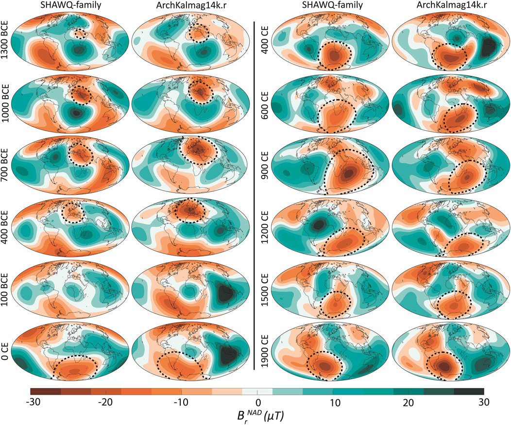
Figure 1. Snapshots of the non-axial radial component
Some other aspects must be highlighted about the LIANAA and SANAA features. On one hand, although negative patches of the radial component represent both anomalies, this implies a different behavior for each anomaly due to their hemispherical location. The LIANAA is located at the northern hemisphere (where the full harmonic radial component is dominantly negative). Consequently, this negative anomaly reinforces the radial component and thus, an intensity maximum at the Earth’s surface is expected. However, the SANAA is located at the southern hemisphere where the full harmonic radial component is positive. Then, the negative anomaly reduces the radial component and therefore low intensities are expected in this region (see Supplementary Figure S3 of Supplementary Material). On the other hand, the reliability of the used global paleo-reconstructions hardly depends, not only on the parametrization and on priors used during the inversion process, but also on the quality and spatial and temporal distribution of the TRM data (Campuzano et al., 2019; Schanner et al., 2022). Although it is still necessary to improve the archeomagnetic database (Supplementary Material, Supplementary Figure S4), with the present information it is possible to make here an approach to investigate the evolution of these anomalies, which can also contribute to guiding future archeomagnetic studies (key regions, periods, etc.).
Following De Santis and Qamili (2010), we assume that, locally, the anomaly features (LIANAA and SANAA) can be simply modelled by means of the non-axial radial component (Equation 1) as a local monopolar source
The expression of
where

Figure 2. Sketch of the field created in surface by a positive monopole located in M defined by colatitude
Assuming an insulate mantle, we can calculate the monopole field in any point of the space outside the core (see Figure 2). The distance between two points defined by its geocentric spherical coordinates can be calculated as:
where
where
Equation 6 is used to model the LIANAA and SANAA within the temporal windows where they are defined (i.e. 1300 BCE – 200 BCE for the LIANAA, and the last 2000 years for the SANAA). For a certain time t, the monopole approach has been applied as follows.
• We first synthetize
• Once the anomaly patch is identified, we proceed to determine the center of the anomaly and its circular boundaries to accurately model the non-axial radial component within this region through Equation 6. Given that the anomaly patch undergoes temporal movement, and its area continually expands or contracts, these parameters (the center and size of the spherical cap containing the anomaly patch) will vary over time. In Supplementary Figure S5 of Supplementary Material, we show the LIANAA center location from 1300 BCE to 200 BCE and the SANAA center location for the last 2000 years. Then, a circular grid around this center, which radius is named as the semi-aperture, defines the anomaly contour line. Both SANAA and LIANAA patches are defined as negative anomalies of
• Finally, after properly delimiting the circular grid within the anomaly patch for each time t, we use Equation 6 to estimate the unknown parameters of the monopole field:
In Figure 3, we show some snapshots of LIANAA and SANAA in a spherical cap defined by the semi-aperture for both SHAWQ-family and ArchKalmag14k.r models. In addition, in Supplementary Figure S6 of Supplementary Material, we show the time evolution of the values of the semi-aperture for target time windows and both paleo-reconstructions. As expected, the aperture for LIANAA presents lower values than for the SANAA, since the LIANAA is characterized by smaller spatial wavelengths than the SANAA. Moreover, for the LIANAA period, the ArchKalmag14k.r model provides larger apertures than the SHAWQ-family model. For the SANAA period, both models present similar apertures, except for the time interval 550–1100 CE, where the ArchKalmag14k.r presents lower values. Finally, it is important to note that the ArchKalmag14k.r model did not properly define the anomaly patches of LIANAA from 1200 BCE to 1100 BCE and, thus, there are no results during this period for this model.
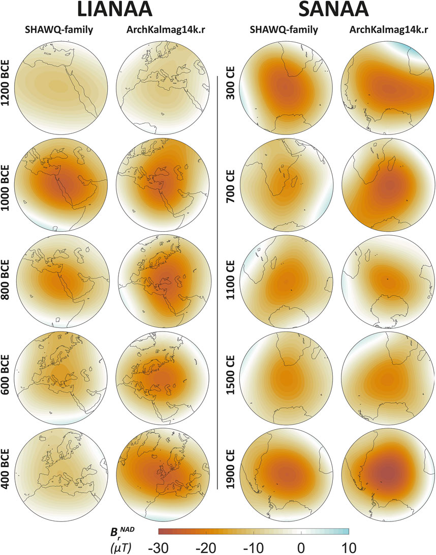
Figure 3. Snapshots of
It is worth noting that our monopole approach simplifies the geometry of the local
Some aspects are crucial for the physical interpretation of the equivalent monopole source for LIANAA and SANAA. In the work of O’Brien and Parker (1994) they test the best depth of the monopoles to fit the radial field at the CMB, considering they should be located in the magnetic source region (Earth’s outer core). Here, we implement a test fixing different values of
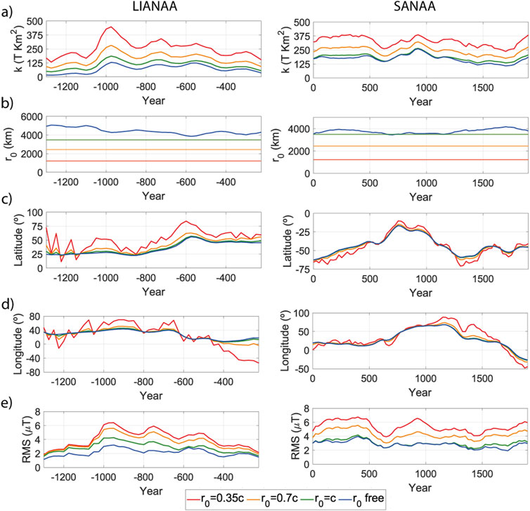
Figure 4. (a–d) Parameters of the monopole model and (e) RMS between the monopole and non-axial radial fields on Earth’s surface for the LIANAA (left) and SANAA (right) using the SHAWQ-family model for different values of
The free-
In Figure 4B, the monopole strength (parameter k) shows high dependence with the depth of the monopole. As expected, a deeper monopole requires higher strength to create similar radial field values at Earth’s surface. Mean k values range between 75 μT and 255 μT for the LIANAA, and between 170 μT and 325 μT for the SANAA, for the most superficial (free-
No significant differences are observed for the latitude
To quantify the robustness of the fitting, the RMS misfit as a function of time is plotted in Figure 4E. For both target time-windows, the RMS misfit increases for a deeper monopole (up to RMS of 6 μT and 7 μT for the LIANAA and SANAA, respectively). This behavior is related with the spatial wavelength of each non-axial anomaly. When the monopole is deeper,
Although the best fit (lower RMS) of the non-axial patches is obtained by letting
Once the depth of the monopole is determined (
Afterwards, we analyze our monopole model (
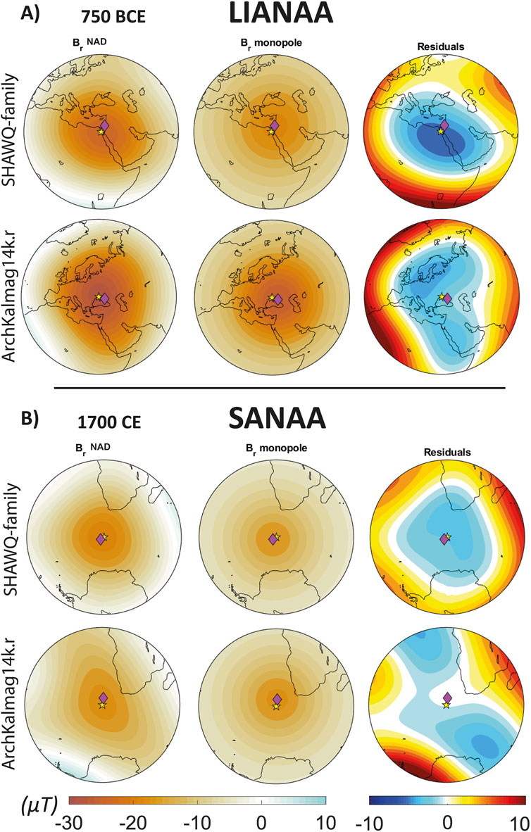
Figure 5. (a)
Taking into account the patch shapes, the SHAWQ-family model shows a LIANAA elongated along the longitude and a more circular SANAA, while the ArchKalmag14k.r model reveals circular-like anomalies latitudinally elongated for both LIANAA and SANAA. In all the cases, their respective monopole models (center column in Figure 5) present, as expected, perfect circular geometries with minimum values similar to those given by the paleo-reconstructions. In Figure 5, we also plot the projection on Earth’s surface of the monopole location (yellow star) and the center of the anomalous
Residuals are constrained within the range of −8–10 µT within the circular patches (right column in Figure 5) and highlight specific regions where the monopoles underestimate or overestimate the non-axial radial field data, offering valuable insights into the non-axial field geometry of these anomalies. As a broader view, the monopole underestimates the field in the center of the patch and overestimates it around the anomaly, due to the larger spatial wavelength of the monopole radial field.
Figure 6 summarizes the monopole parameters for the LIANAA given by both paleo-reconstructions. The ArchKalmag14k.r model reproduces higher values of
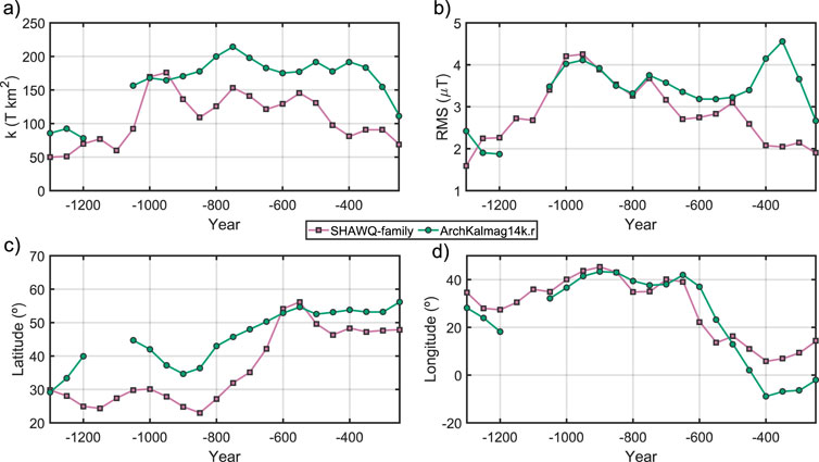
Figure 6. Time evolution of the optimal parameters (a) k, (c)
The RMS between
During the first peak of the LIAA event (around 950 BCE), the monopole is located at low latitudes with mean values of around 25°N for SHAWQ-family and around 30°N for ArchKalmag14k.r (see Figure 6C). After that, a northward drift is observed reaching latitudes over 50°N around 600 BCE. After 550 BCE the latitude remains stable around 52°N for ArchKalmag14k.r and a bit lower (45°N) for SHAWQ-family. The monopole longitude (Figure 6D) shows similar results during this period for both SHAWQ-family and ArchKalmag14k.r models. The LIANAA longitude remains steady at approximately 40°E during the LIAA event (i.e., 1000 BCE – 700 BCE). After that, the monopole source exhibits a westward drift to the center of Europe as indicated by the archeointensity data (Osete et al., 2020; Rivera et al., 2023).
The monopole parameters for the SANAA time interval (last two millennia) are plotted in Figure 7. To evaluate the results of the monopole model using the reconstructions based on paleomagnetic data (SHAWQ-family and ArchKalmag14k.r), we also estimate the monopole parameters using a historical geomagnetic field model developed by using exclusively historical and instrumental data. The chosen historical model is the COV-OBS.x2 (Huder et al., 2020) that runs from 1840 CE to 2000 CE (orange diamonds in Figure 7). In general, before historical era, the monopole parameters for both SHAWQ-family and ArchKalmag14k.r seem to match better during the second millennium CE, related with a better reliability of the models and definition of the SANAA patch (see Movies S1-S2 of Supplementary Material). During the historical era (from 1840 CE), the monopole parameters for SHAWQ-family and ArchKalmag14k.r agree with COV-OBS.x2 model, with better agreement for SHAWQ-family model (see Supplementary Figure S12 in Supplementary Material).
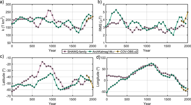
Figure 7. Time evolution of the optimal parameters (a) k, (c)
In Figure 7A, the parameter
The RMS values stay low (2 μT–5 µT) for both paleo-reconstructions during the whole period (Figure 7B). For two epochs, the RMS show higher values: first, during the first 500 years, in particular for ArchKalmag14k.r, due to the lack of data for this period and worse definition of the SANAA patch; second, from 1700 CE to present all models, archeomagnetic and instrumental, agree with an increase of RMS values, related with the present non-circular geometry of SAA.
The latitude of the monopole shows a low variability around 40° for the whole period (Figure 7C). SHAWQ-family and ArchKalmag14k.r show agreement, with more northern latitudes for SHAWQ-family during the first 1,300 years. Both models show that the source comes from the southern regions, drifts northwards during the first millennium CE and, afterwards, shows a fast southern drift from 1000 CE to 1200 CE. During the last 700 years, the monopole stays between 60°S and 40°S with a slight northwards displacement till 1800 and drifting to southern latitudes during historical era in agreement with COV-OBSx2 model. The monopole longitude (Figure 7D) agrees for SHAWQ-family and ArchKalmag14k.r models and is characterized by eastward drift till the beginning of the second millennium CE, reaching ∼70°E between 1000 CE and 1200 CE. From then, both models show a westward drift linked with the well-known westward movement characteristic of the SAA for the last 400 years. The instrumental model COV-OBSx2 shows that this westward drift stops around 50°W in 1950 CE and change the drifting direction eastwards. This is linked with the elongation and appearance of a second minimum of the SAA for the present field (e.g., Finlay et al., 2020; among others).
Some important geomagnetic features observed at the Earth’s surface are modulated by the transitional region between the lower mantle and the upper part of the outer core (Kirscher et al., 2018; Terra-Nova et al., 2019; Korte et al., 2022). In this context, lower mantle heterogeneities seem to play an important role in some geomagnetic features. This is the case of the anomaly features analyzed in this work: the SAA is suggested to be related to heterogeneous structure of the lower mantle, not only for the Holocene but also for longer timescales (Tarduno et al., 2015; Shah et al., 2016; Trindade et al., 2018; Hare et al., 2018; Terra-Nova et al., 2019; He et al., 2021; Nilsson et al., 2022) extending even to millions of years (Engbers et al., 2020; de Oliveira et al., 2024). These structures of the low mantle related to the SAA are characterized by low seismic S-wave anomaly and are called Large Low Shear Velocity Provinces (LLSVPs). LLSVPs cover around 20% of the core mantle boundary (under Africa and South-Central Pacific) and extend up to around 1,000 km above the CMB. They are mainly dominated by thermal effects in the mantle but also compositional, thus contain a significant component of chemically dense material (see Davies et al., 2015 for a review). However, as far as we know, no connection with low mantle heterogeneities has been discovered yet for the LIAA event. In order to provide more information about the connection between the SAA and the African LLSVP, and to see if the LIAA is also connected with this heterogeneous region, here we compare the position of the anomaly monopoles for LIANAA and SANAA with the African LLSVP extension.
Tarduno et al. (2015) suggested that anomalies could be created in the edges of the LLSVPs due to sharp structural gradients that can be expected to stimulate the formation of small-scale vortices in the flow. This will develop an upward component and allow a reversed polarity flux to leak upward. In that work, they propose that the summation and upward continuation of these reversed and normal patches might result in the SAA low field strengths in surface. The African LLSVP is thought to be older than 100 million years and the sides (due to lower mantle viscosity of 1 cm/yr (Hager, 1984)) relatively unchanged for 1–10 Myr. Thus, the present geometry of these mantle features should have been constant for the last 10 Myr which suggests a recurrence of these anomalies. This relationship between the edges of the LLSVPs and surface intensity anomalies in the geomagnetic field has also been found in other anomalies like the West Pacific Anomaly (WPA) present during 16th and 19th century CE in the western edge of the Pacific LLSVP (He et al., 2021; Tema et al., 2022).
In Figure 8A, we plot the location of the monopole for the SANAA and LIANAA using the SHAWQ-family and ArchKalmag14k.r covering the last 3,300 years over a contour of a seismic tomography model at the CMB, constraining the African LLSVP. Following Korte et al. (2022), we use as a proxy for the LLSVP at the CMB an average model using S10mean (Doubrovine et al., 2016) which is itself an average from 10 models, SP12RTS-S (Koelemeijer et al., 2016), SEISGLOB2 (Durand et al., 2017) and TX2019salb-S (Lu et al., 2019). To plot the contour of the African LLSVP, we first normalize the amplitude of the velocity models before taking the average (done by the tool SubMachine, Hosseini et al. (2018)), so the velocity anomaly values range between −1 and 1. Values below the average (negative values) are considered to define the LLSVPs. In Figure 8A, we also represent (by orange diamonds) the monopole centers of the instrumental model COV-OBSx.2 that show the SANAA evolution for the present field. The monopole centers for all models seem to move in areas with low velocity anomaly in absolute value, that is, the monopoles are located around the edges of the African LLSVP.
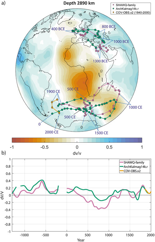
Figure 8. (a) Trajectories of the monopole for the SANAA and LIANAA for SHAWQ-family, ArchKalmag14k.r and COV-OBS.x2 models, plotted every 50 years. The colormap shows the normalized S-velocity at the CMB, at 2,890 km depth, obtained from the average of selected tomography models. The negative velocity anomaly values (orange colors) characterize the African LLSVP. (b) Normalized S-velocity at the CMB in the location of the monopole for the same models. Note that no monopole is solved for ArchKalmag14k.r model from 1200 BCE to 1100 BCE and the transition between both anomalies from 200 BCE to 0 CE. Instrumental model COV-OBS.x2, only from 1840 CE to 2000 CE.
In addition, for deeper analysis, we calculate the S-velocity anomaly at the CMB in the location of the monopoles for SHAWQ-family, ArchKalmag14k.r and COV-OBS.x2 (for instrumental period). In Figure 8B, we plot the time-curves of the S-velocity anomaly for LIANAA and SANAA. The S-velocity anomaly values remain low, between −0.2 and 0.2, only reaching absolute values over 0.3 around 700–600 BCE for both models and 800 CE for SHAWQ-family. The monopoles for LIANAA are mostly located in positive s-velocity anomaly regions, in contrast with SANAA that show negative S-velocities during the first millennium CE. Nevertheless, in general, the S-velocity anomaly values remain close to 0 for both anomalies and models. These results show that both LIANAA and SANAA sources seem to remain close to the edges of the LLSVP-related positive anomaly regions.
The axisymmetric axial dipole can mask some features of the field, which shows the importance of studying the non-axial components. In this work, we have analyzed the SAA and LIAA by examining the non-axial radial field in Earth’s surface using the SHAWQ-family and ArchKalmag14k.r archeomagnetic models for the Holocene. We have focused on two negative radial patches: one is present from 1300 BCE to 200 CE, linked with the LIAA event and the high intensities in Europe around the fifth century BCE; the other patch is present in the south hemisphere during the last 2000 years, linked with the SAA during the last 400 years. This last patch seems to be present before 1000 CE, preceding the emergence of the SAA, a topic still under debate. Both SHAWQ-family and ArchKalmag14k.r models agree with the presence of these non-axial patches, although discrepancies in their shape and location arise due to the temporal and spatial heterogeneity of the database.
In our work, we have examined these anomalies by fitting the negative patches of the non-axial radial field using an equivalent monopole source. It is worth noting that a magnetic monopole lacks direct physical interpretation, but it can offer detailed insights into the location, extent, morphology and evolution of these anomalies. The monopole model reproduces the non-axial patches locally with residuals under archeomagnetic data uncertainty and shows good agreement between the used models. Here, it is important to point out certain limitations: the monopole strength exhibits notable sensitivity to the monopole location
Recent studies suggest that anomalies in the past and present geomagnetic field might be mantle driven and their location seems to be related with the lower mantle structure. This link implies that anomalies might be a recurrent or persistent feature of the field. In our work, we show that the sources of the LIAA and SAA non-axial patches seems to move around the edges of the African LLSVP. Recent works show that SAA might be an anomaly influenced by mantle heterogeneities and we suggest that other features as LIAA, which source seems to move around the northeast edge of the African LLSVP, can also be mantle related.
The original contributions presented in the study are included in the article/Supplementary Material, further inquiries can be directed to the corresponding author.
PR: Conceptualization, Data curation, Formal Analysis, Investigation, Methodology, Software, Validation, Visualization, Writing–original draft, Writing–review and editing. FP-C: Conceptualization, Funding acquisition, Investigation, Methodology, Project administration, Resources, Software, Supervision, Validation, Visualization, Writing–original draft, Writing–review and editing. AD: Conceptualization, Investigation, Methodology, Writing–original draft, Writing–review and editing. SC: Investigation, Methodology, Writing–original draft, Writing–review and editing. GC: Methodology, Writing–original draft, Writing–review and editing. MO: Conceptualization, Funding acquisition, Investigation, Methodology, Project administration, Resources, Supervision, Validation, Visualization, Writing–original draft, Writing–review and editing.
The author(s) declare that financial support was received for the research, authorship, and/or publication of this article. This research was funded by Spanish Ministry of Universities (FPU18/01567) and Spanish Ministry of Science and Innovation (PID 2020-117105RB-I00, PID 2020-113316GB-100 and CSIC i-LINK-22057).
The authors are grateful to the Spanish Ministry of Science and Innovation for supporting this research through the project PULSES.5K (PID 2020-117105RB-I00), SUMATE (PID 2020-113316GB-100) and CSIC i-LINK-22057. PR thanks the Spanish Ministry of Universities (FPU18/01567) for the funding of his PhD. We also acknowledge the Editors of this journal and the two referees for the improvement of this manuscript.
The authors declare that the research was conducted in the absence of any commercial or financial relationships that could be construed as a potential conflict of interest.
The author(s) declare that no Generative AI was used in the creation of this manuscript.
All claims expressed in this article are solely those of the authors and do not necessarily represent those of their affiliated organizations, or those of the publisher, the editors and the reviewers. Any product that may be evaluated in this article, or claim that may be made by its manufacturer, is not guaranteed or endorsed by the publisher.
The Supplementary Material for this article can be found online at: https://www.frontiersin.org/articles/10.3389/feart.2025.1515777/full#supplementary-material
SAA, South Atlantic Anomaly; LIAA, Levantine Iron Age Anomaly; LLSVP, Low Large Shear Velocity Province; TRM, Thermoremanent magnetization; CMB, Core-mantle boundary; SHA, Spherical Harmonic Analysis; LIANAA, Levantine Iron Age Non-Axial anomaly; SANAA, South Atlantic Non-Axial Anomaly; RMS, Roots Mean Square error.
Amit, H., Terra-Nova, F., Lézin, M., and Trindade, R. I. (2021). Non-monotonic growth and motion of the South atlantic anomaly. Earth, Planets Space 73, 38–10. doi:10.1186/s40623-021-01356-w
Ben-Yosef, E., Tauxe, L., Levy, T. E., Shaar, R., Ron, H., and Najjar, M. (2009). Geomagnetic intensity spike recorded in high resolution slag deposit in Southern Jordan. Earth Planet. Sci. Lett. 287, 529–539. doi:10.1016/j.epsl.2009.09.001
Brown, M. C., Donadini, F., Korte, M., Nilsson, A., Korhonen, K., Lodge, A., et al. (2015). GEOMAGIA50.v3: 1. general structure and modifications to the archeological and volcanic database. Earth Planets Space 67, 83. doi:10.1186/s40623-015-0232-0
Cafarella, L., De Santis, A., and Meloni, A. (1992). The historical Italian geomagnetic data catalogue. Rome: Ist. Naz. di Geofis. e Vulcanol., 160.
Campuzano, S. A., Gómez-Paccard, M., Pavón-Carrasco, F. J., and Osete, M. L. (2019). Emergence and evolution of the South Atlantic Anomaly revealed by the new paleomagnetic reconstruction SHAWQ2k. Earth Planet. Sci. Lett. 512, 17–26. doi:10.1016/j.epsl.2019.01.050
Davies, C., and Constable, C. (2017). Geomagnetic spikes on the core-mantle boundary. Nat. Commun. 8, 15593. doi:10.1038/ncomms15593
Davies, D. R., Goes, S., and Lau, H. C. P. (2015). “Thermally dominated deep mantle LLSVPs: a review,” in The Earth’s heterogeneous mantle. Editors A. Khan, and F. Deschamps (Cham: Springer International Publishing), 441–477. doi:10.1007/978-3-319-15627-9_14
de Oliveira, W. P., Hartmann, G. A., Terra-Nova, F., Pasqualon, N. G., Savian, J. F., Lima, E. F., et al. (2024). Long-term persistency of a strong non-dipole field in the South Atlantic. Nat. Commun. 15, 9447. doi:10.1038/s41467-024-53688-2
De Santis, A., and Qamili, E. (2010). Equivalent monopole source of the geomagnetic South Atlantic anomaly. Pure Appl. Geophys. 167, 339–347. doi:10.1007/s00024-009-0020-5
Doubrovine, P. V., Steinberger, B., and Torsvik, T. H. (2016). A failure to reject: testing the correlation between large igneous provinces and deep mantle structures with edf statistics. Geochem. Geophys. Geosyst. 17, 1130–1163. doi:10.1002/2015gc006044
Durand, S., Debayle, E., Ricard, Y., Zaroli, C., and Lambotte, S. (2017). Confirmation of a change in the global shear velocity pattern at around 1000 km depth. Geophys. J. Int. 211, 1628–1639. doi:10.1093/gji/ggx405
Engbers, Y. A., Biggin, A. J., and Bono, R. K. (2020). Elevated paleomagnetic dispersion at Saint Helena suggests long-lived anomalous behavior in the South Atlantic. Proc. Natl. Acad. Sci. 117, 18258–18263. doi:10.1073/pnas.2001217117
Finlay, C. C., Aubert, J., and Gillet, N. (2016). Gyre-driven decay of the Earth’s magnetic dipole. Nat. Commun. 7, 10422. doi:10.1038/ncomms10422
Finlay, C. C., Kloss, C., Olsen, N., Hammer, M. D., Tøffner-Clausen, L., Grayver, A., et al. (2020). The CHAOS-7 geomagnetic field model and observed changes in the South Atlantic Anomaly. Earth Planets Space 72, 156. doi:10.1186/s40623-020-01252-9
Gauss, C. F. (1833). Intensitas vis magneticae terrestris ad mensuram absolutam revocata Göttingen, Germany: Dieterich.
Hager, B. H. (1984). Subducted slabs and the geoid- Constraints on mantle rheology and flow. J. Geophys. Res. 89, 6003–6015. doi:10.1029/jb089ib07p06003
Hare, V. J., Tarduno, J. A., Huffman, T., Watkeys, M., Thebe, P. C., Manyanga, M., et al. (2018). New archeomagnetic directional records from Iron age southern Africa (ca. 425–1550 CE) and implications for the South atlantic anomaly. Geophys. Res. Lett. 45, 1361–1369. doi:10.1002/2017GL076007
Hartmann, G. A., and Pacca, I. G. (2009). Time evolution of the South atlantic magnetic anomaly. An. Acad. Bras. Ciênc. 81, 243–255. doi:10.1590/S0001-37652009000200010
He, F., Wei, Y., Maffei, S., Livermore, P. W., Davies, C. J., Mound, J., et al. (2021). Equatorial auroral records reveal dynamics of the paleo-West Pacific geomagnetic anomaly. Proc. Natl. Acad. Sci. 118, e2026080118. doi:10.1073/pnas.2026080118
Hodder, B. M. (1982). Monopoly. Geophys. J. Int. 70, 217–228. doi:10.1111/j.1365-246X.1982.tb06401.x
Hosseini, K., Matthews, K. J., Sigloch, K., Shephard, G. E., Domeier, M., and Tsekhmistrenko, M. (2018). Submachine: web-based tools for exploring seismic tomography and other models of Earth’s deep interior. Geochem. Geophys. Geosyst. 19, 1464–1483. doi:10.1029/2018gc007431
Huder, L., Gillet, N., Finlay, C. C., Hammer, M. D., and Tchoungui, H. (2020). COV-OBS.x2: 180 years of geomagnetic field evolution from ground-based and satellite observations. Earth Planets Space 72, 160. doi:10.1186/s40623-020-01194-2
Jackson, A., and Finlay, C. (2015). Geomagnetic secular variation and its applications to the core. Phys. Sci., 137, 184. doi:10.1016/B978-0-444-53802-4.00099-3
Jackson, A., Jonkers, A. R. T., and Walker, M. R. (2000). Four centuries of geomagnetic secular variation from historical records. Phys. Eng. Sci. 358, 957–990. doi:10.1098/rsta.2000.0569
Jonkers, A. R., Jackson, A., and Murray, A. (2003). Four centuries of geomagnetic data from historical records. Rev. Geophys. 41 (2). doi:10.1029/2002rg000115
Kirscher, U., Winklhofer, M., Hackl, M., and Bachtadse, V. (2018). Detailed Jaramillo field reversals recorded in lake sediments from Armenia – lower mantle influence on the magnetic field revisited. Earth Planet. Sci. Lett. 484, 124–134. doi:10.1016/j.epsl.2017.12.010
Koelemeijer, P., Ritsema, J., Deuss, A., and Van Heijst, H.-J. (2016). Sp12rts: a degree-12 model of shear-and compressional-wave velocity for Earth’s mantle. Geophys. J. Int. 204, 1024–1039. doi:10.1093/gji/ggv481
Korte, M., Constable, C. G., Davies, C. J., and Panovska, S. (2022). Indicators of mantle control on the geodynamo from observations and simulations. Front. Earth Sci. 10, 957815. doi:10.3389/feart.2022.957815
Korte, M., Donadini, F., and Constable, C. G. (2009). Geomagnetic field for 0–3 ka: 2. A new series of time-varying global models. Geochem. Geophys. Geosystems 10, 2008GC002297. doi:10.1029/2008GC002297
Livermore, P. W., Fournier, A., and Gallet, Y. (2014). Core-flow constraints on extreme archeomagnetic intensity changes. Earth Planet. Sci. Lett. 387, 145–156. doi:10.1016/j.epsl.2013.11.020
Livermore, P. W., Gallet, Y., and Fournier, A. (2021). Archeomagnetic intensity variations during the era of geomagnetic spikes in the Levant. Phys. Earth Planet. Inter. 312, 106657. doi:10.1016/j.pepi.2021.106657
Lu, C., Grand, S. P., Lai, H., and Garnero, E. J. (2019). Tx2019slab: a new p and s tomography model incorporating subducting slabs. J. Geophys. Res. Solid Earth 124, 11549–11567. doi:10.1029/2019jb017448
Macmillan, S., and Maus, S. (2005). International geomagnetic reference field—the tenth generation. Earth Planets Space 57, 1135–1140. doi:10.1186/BF03351896
McLeod, M. G., and Coleman, P. J. (1980). Spatial power spectra of the crustal geomagnetic field and J. geophys. Res. Phys. Earth planet. Int. 69, 2631. doi:10.1016/0031-9201(80)90002-3
Nilsson, A., and Suttie, N. (2021). Probabilistic approach to geomagnetic field modelling of data with age uncertainties and post-depositional magnetisations. Phys. Earth Planet. Inter. 317, 106737. doi:10.1016/j.pepi.2021.106737
Nilsson, A., Suttie, N., Stoner, J. S., and Muscheler, R. (2022). Recurrent ancient geomagnetic field anomalies shed light on future evolution of the South Atlantic Anomaly. Proc. Natl. Acad. Sci. 119, e2200749119. doi:10.1073/pnas.2200749119
O’Brien, M. S., and Parker, R. L. (1994). Regularized geomagnetic field modelling using monopoles. Geophys. J. Int. 118, 566–578. doi:10.1111/j.1365-246X.1994.tb03985.x
Olson, P., and Amit, H. (2006). Changes in earth’s dipole. Naturwissenschaften 93, 519–542. doi:10.1007/s00114-006-0138-6
Olson, P., Deguen, R., Rudolph, M. L., and Zhong, S. (2015). Core evolution driven by mantle global circulation. Phys. Earth Planet. Inter. 243, 44–55. doi:10.1016/j.pepi.2015.03.002
Osete, M. L., Molina-Cardín, A., Campuzano, S. A., Aguilella-Arzo, G., Barrachina-Ibañez, A., Falomir-Granell, F., et al. (2020). Two archaeomagnetic intensity maxima and rapid directional variation rates during the Early Iron Age observed at Iberian coordinates. Implications on the evolution of the Levantine Iron Age Anomaly. Earth Planet. Sci. Lett. 533, 116047. doi:10.1016/j.epsl.2019.116047
Pavón-Carrasco, F. J., and De Santis, A. (2016). The South Atlantic anomaly: the key for a possible geomagnetic reversal. Front. Earth Sci. 4, 40. doi:10.3389/feart.2016.00040
Rivera, P., Pavón-Carrasco, F. J., and Osete, M. L. (2023). Modeling geomagnetic spikes: the levantine Iron age anomaly. Earth Planets Space 75, 133. doi:10.1186/s40623-023-01880-x
Rivero-Montero, M., Gómez-Paccard, M., Kondopoulou, D., Tema, E., Pavón-Carrasco, F. J., Aidona, E., et al. (2021). Geomagnetic field intensity changes in the central mediterranean between 1500 BCE and 150 CE: implications for the levantine Iron age anomaly evolution. Earth Planet. Sci. Lett. 557, 116732. doi:10.1016/j.epsl.2020.116732
Schanner, M., Korte, M., and Holschneider, M. (2022). ArchKalmag14k: a kalman-filter based global geomagnetic model for the Holocene. J. Geophys. Res. Solid Earth 127, e2021JB023166. doi:10.1029/2021JB023166
Shaar, R., Ben-Yosef, E., Ron, H., Tauxe, L., Agnon, A., and Kessel, R. (2011). Geomagnetic field intensity: how high can it get? How fast can it change? Constraints from Iron Age copper slag. Earth Planet. Sci. Lett. 301, 297–306. doi:10.1016/j.epsl.2010.11.013
Shaar, R., Gallet, Y., Vaknin, Y., Gonen, L., Martin, M. A. S., Adams, M. J., et al. (2022). Archaeomagnetism in the levant and mesopotamia reveals the largest changes in the geomagnetic field. J. Geophys. Res. Solid Earth 127, e2022JB024962. doi:10.1029/2022JB024962
Shaar, R., Tauxe, L., Ron, H., Ebert, Y., Zuckerman, S., Finkelstein, I., et al. (2016). Large geomagnetic field anomalies revealed in bronze to Iron age archeomagnetic data from tel megiddo and tel hazor, Israel. Earth Planet. Sci. Lett. 442, 173–185. doi:10.1016/j.epsl.2016.02.038
Shah, J., Koppers, A. A. P., Leitner, M., Leonhardt, R., Muxworthy, A. R., Heunemann, C., et al. (2016). Palaeomagnetic evidence for the persistence or recurrence of geomagnetic main field anomalies in the South Atlantic. Earth Planet. Sci. Lett. 441, 113–124. doi:10.1016/j.epsl.2016.02.039
Tarduno, J. A., Watkeys, M. K., Huffman, T. N., Cottrell, R. D., Blackman, E. G., Wendt, A., et al. (2015). Antiquity of the South Atlantic Anomaly and evidence for top-down control on the geodynamo. Nat. Commun. 6, 7865. doi:10.1038/ncomms8865
Tema, E., Santos, Y., Trindade, R., Hartmann, G. A., Hatakeyama, T., Terra-Nova, F., et al. (2022). Archaeointensity record of weak field recurrence in Japan: new data from Late Yayoi and Kofun ceramic artifacts. Geophys. J. Int. ggac498. doi:10.1093/gji/ggac498
Terra-Nova, F., Amit, H., and Choblet, G. (2019). Preferred locations of weak surface field in numerical dynamos with heterogeneous core–mantle boundary heat flux: consequences for the South Atlantic Anomaly. Geophys. J. Int. 217, 1179–1199. doi:10.1093/gji/ggy519
Terra-Nova, F., Amit, H., Hartmann, G. A., Trindade, R. I., and Pinheiro, K. J. (2017). Relating the South atlantic anomaly and geomagnetic flux patches. Phys. Earth Planet. Interiors 266, 39–53. doi:10.1016/j.pepi.2017.03.002
Keywords: South Atlantic Anomaly, Levantine Iron Age Anomaly, monopole approach, archeomagnetism, paleomagnetic reconstruction models, Low Large Shear Velocity Provinces
Citation: Rivera P, Pavón-Carrasco FJ, De Santis A, Campuzano SA, Cianchini G and Osete ML (2025) Magnetic core field anomalies in the non-axial field during the last 3300 years: approach with an equivalent monopole source. Front. Earth Sci. 13:1515777. doi: 10.3389/feart.2025.1515777
Received: 23 October 2024; Accepted: 03 February 2025;
Published: 27 February 2025.
Edited by:
Eric Font, University of Coimbra, PortugalReviewed by:
Sanja Panovska, GFZ German Research Centre for Geosciences, GermanyCopyright © 2025 Rivera, Pavón-Carrasco, De Santis, Campuzano, Cianchini and Osete. This is an open-access article distributed under the terms of the Creative Commons Attribution License (CC BY). The use, distribution or reproduction in other forums is permitted, provided the original author(s) and the copyright owner(s) are credited and that the original publication in this journal is cited, in accordance with accepted academic practice. No use, distribution or reproduction is permitted which does not comply with these terms.
*Correspondence: Pablo Rivera, cGFibG9yaXZAdWNtLmVz
†ORCID: Pablo Rivera, orcid.org/0000-0001-7092-344X; F. Javier Pavón-Carrasco, orcid.org/0000-0001-5545-3769; Angelo De Santis, orcid.org/0000-0002-3941-656X; Saioa A. Campuzano, orcid.org/0000-0001-7047-5704; Gianfranco Cianchini, orcid.org/0000-0003-2832-0068; María Luisa Osete, orcid.org/0000-0001-5767-2877
Disclaimer: All claims expressed in this article are solely those of the authors and do not necessarily represent those of their affiliated organizations, or those of the publisher, the editors and the reviewers. Any product that may be evaluated in this article or claim that may be made by its manufacturer is not guaranteed or endorsed by the publisher.
Research integrity at Frontiers
Learn more about the work of our research integrity team to safeguard the quality of each article we publish.