Tunnel squeezing prediction based on partially missing dataset and optimized machine learning models

Accurate prediction of tunnel squeezing, one of the common geological hazards during tunnel construction, is of great significance for ensuring construction safety and reducing economic losses. To achieve precise prediction of tunnel squeezing, this study constructed six reliable machine learning (ML) classification models for this purpose, including Support Vector Machine (SVM), Random Forest (RF), Decision Tree (DT), Extreme Gradient Boosting (XGBoost), Light Gradient Boosting Machine (LGBM), and K-Nearest Neighbors (KNN). The parameters of these 6 ML models were optimized using the Whale Optimization Algorithm (WOA) in conjunction with five-fold cross-validation. A total of 305 tunnel squeezing sample data were collected to train and test the models. KNN and Synthetic Minority Over-sampling Technique (SMOTE) methods were employed to handle the missing and imbalanced data sets. An input feature system for tunnel squeezing prediction was established, comprising tunnel burial depth (H), tunnel diameter (D), strength-to-stress ratio (SSR), and support stiffness (K). The XGBoost model optimized with WOA demonstrated the highest prediction accuracy of 0.9681. The SHAP method was utilized to interpret the XGBoost model, indicating that the contribution rank of the input features to tunnel squeezing prediction was SSR > K > D > H, with average SHAP values of 2.93, 1.49, 0.82, and 0.69, respectively. The XGBoost model was applied to predict tunnel squeezing in 10 sections of the Qinghai Huzhu Beishan Tunnel. The prediction results were highly consistent with the actual outcomes.

1 Introduction

As a crucial component of modern infrastructure construction, the safety and stability of tunnel engineering are directly related to the safety of human lives and properties as well as the harmonious development of society. Nowadays, tunnel engineering is gradually advancing towards deeper levels, encountering increasingly complex geological conditions and environments. When tunnels traverse weak rock strata and lack sufficient support strength, they are prone to compressive deformation under high in-situ stress, leading to significant delays in construction schedules and, in more severe cases, potentially causing accidents involving loss of life (Hoek and Marinos, 2000; Mikaeil et al., 2019; Zhu et al., 2019). The squeezing behavior of surrounding rock can be described as large deformations that vary over time during tunnel excavation. Its essence is related to creep resulting from exceeding the ultimate shear stress, and it often occurs around tunnels subjected to high in-situ stresses (Dwivedi et al., 2013; Jain and Rao, 2022; Singh et al., 2007). Therefore, conducting in-depth research on tunnel squeezing prediction methods and improving their accuracy and timeliness are of great significance for ensuring the safe construction and long-term operation of tunnel engineering.

Since the 1990s, tunnel squeezing prediction has been extensively studied, and scholars have proposed various methods for predicting tunnel squeezing, including empirical methods, semi-empirical methods, and theoretical methods (Aydan et al., 1993; Ghiasi et al., 2012; Hoek, 2001; Panthi, 2013; Singh et al., 1992). Traditional estimation methods based on empirical and semi-empirical approaches include the stress ratio method, burial depth method, and deformation method. Among them, the stress ratio method encompasses ratios such as the ratio of surrounding rock strength to in-situ stress and the ratio of uniaxial compressive strength to in-situ stress (Aydan et al., 1993; Martin et al., 2011). The burial depth method determines the occurrence of squeezing based on the correlation between the burial depth of the tunnel and the quality of the surrounding rock (Goel et al., 1995). The deformation method assesses the degree of squeezing by establishing a functional relationship between the relative deformation of the tunnel and its influencing factors (Dwivedi et al., 2013). In this method, the evaluation criteria proposed by Hoek have been widely accepted (Hoek and Marinos, 2000).

With the continuous development and advancement of computer technology, ML techniques have garnered significant attention in the field of tunnel construction due to their potential in data processing and pattern recognition. Ye et al. (2022) proposed a back propagation neural network based on time series (TS-BPNN) to realize soil settlement prediction during the subway tunnel construction. Zhou et al. (2023) developed an XGBoost model optimized with golden-sine seagull optimization to predict the maximum surface settlement induced by shield tunneling. Guo et al. (2024) combined the principal component analysis (PCA) and deep belief network (DBN) to achieve performance prediction of hard rock cantilever road header. An et al. (2024) developed 7 ML models for tunnel convergence prediction in drill-and-blast tunnels and conducted model explanation using SHapley Additive exPlanations (SHAP). Zhao et al. (2024) introduced a ML-based method for analyzing real-time TBM excavation data from a major water conservation project, which revealed the dynamic relationships between construction parameters and surrounding rock grades, there by offering an innovative prediction model based on a personalized scoring mechanism. In the domain of tunnel squeezing prediction, ML methods have also been extensively employed and have demonstrated considerable potential. Feng and Jimenez (2015) proposed a Bayesian classifier for predicting squeezing. Zhang et al. (2020) employed a classifier that integrates seven algorithms, including Back Propagation Neural Network (BPNN), Support Vector Machine (SVM), and Decision Tree (DT), among others, to predict tunnel squeezing.Chen et al. (2020) introduced a ML-based framework to probabilistically predict the squeezing intensity and to dynamically update the prediction during tunnel construction. Bo et al. (2023) introduced an ensemble ML model that integrates four different ML classification models, which achieved a prediction accuracy of 98% on the test set. Fathipour-Azar (2022) employed six different ML models to predict squeezing conditions in rock tunnels. However, there are still limitations. Firstly, there is a lack of consideration involving data oversampling to deal with data imbalance. Secondly, the effort to further interpretate the ML model is very limited.

Inspired by the successful application of ML models in tunnel construction-related prediction tasks (An et al., 2024; Bo et al., 2023; Fathipour-Azar, 2022), this paper adopts six different ML models to conduct tunnel squeezing prediction, namely SVM, DT, RF, XGBoost, LightGBM (LGBM), and k-Nearest-Neighbors (KNN). Hyperparameters optimization is significant for ML models to yield accurate prediction. Traditional hyperparameter optimization methods, such as random search and grid search, have certain limitations in terms of optimization efficiency and effectiveness, particularly when faced with complex models and extensive search spaces, where their efficiency significantly declines. To overcome this limitation, this work employs the Whale Optimization Algorithm (WOA) for hyperparameter optimization of the ML models, aiming to enhance their performance.

When dealing with tunnel engineering data, samples often exhibit varying degrees of missingness due to factors such as data sensitivity, technical difficulties in the collection process, and various physical and logical constraints during transmission. This can further lead to ML models failing to capture changes in critical geological, structural, or construction parameters, thereby affecting the predictive capability of the models (Aristiawati et al., 2019; Beretta and Santaniello, 2016; Huang et al., 2020). To address these issues, this paper adopts the k-nearest-neighbor (KNN) imputation method to fill in missing data and the Synthetic Minority Over-sampling Technique (SMOTE) to handle imbalanced datasets.

The objective of this study is to identify the optimal tunnel squeezing prediction model by comparing and analyzing the performance of 6 ML models, aiming to provide a high-precision decision-making tool for tunnel design and construction. Following this, the research focuses on the explanation of the best-performance ML model. The scientific contributions of this paper can be summarized as follows: (1) The adoption of the KNN method to impute missing data and the utilization of SMOTE techniques to handle imbalanced datasets; (2) The construction of 6 ML models for tunnel squeezing prediction with WOA for hyperparameter optimization; (3) The employment of the SHAP method to interpret the optimal ML model, thereby revealing the important contribution of input features.

The remaining of this paper is organized as follows: Section 2 briefly introduces the principles of six classifiers (SVM, RF, DT, XGB, LGBM, KNN), WOA, and SHAP. Section 3 elaborated on the database and the preprocessing techniques. Section 4 presents the construction and analysis of the 6 ML models optimized using the WOA. Furthermore, the input feature contributions of the best-performing WOA-XGBoost model are analyzed using the SHAP method. Section 5 concludes this study and suggests the future work.

2 Methods

2.1 Machine learning algorithms

2.1.1 SVM

Support Vector Machine (SVM) is a supervised learning model rooted in statistical learning theory, widely employed in both classification and regression analysis tasks. Its core concept revolves around identifying a hyperplane in the feature space that separates samples of different classes while maximizing the margin (or gap) between the two classes, thereby enhancing the generalization ability of the classifier. Support Vector Regression (SVM) represents an extension of SVM to regression problems, inheriting the core ideas from SVM in classification and applying them to the prediction of continuous values (Li et al., 2023). The objective of SVM is to minimize both the complexity of the hyperplane (achieved by controlling the norm of the weight vector) and the prediction error (controlled by the ε-insensitive loss function), thereby identifying a regression model with good generalization ability. For nonlinear problems, the fitting equation established by the SVM model can be expressed as Equation 1 (Li and Mei, 2023):

$f\left(z\right)=w^v\phi \left(z\right)+b(1)$

where $w^v$ represents a vector of weights, $\phi \left(z\right)$ describes a function that generates a mapping from the input values to a higher dimensional space, $b$ represents the model error, also known as the bias.

2.1.2 DT

In the field of data science and ML, the Decision Tree has long occupied a pivotal position as a powerful and intuitive method for classification and regression. By simulating the logical reasoning steps in human decision-making processes, DT presents the process of data classification or prediction in a tree-like structure, enabling the analysis and modeling of complex datasets. In classification tasks, internal nodes represent test conditions for feature attributes, which are used to select the best way to split the data; while leaf nodes store the final class labels, indicating the category to which the samples are assigned (Liang et al., 2024). The construction process of a decision tree typically involves two key steps: feature selection and tree pruning. Feature selection aims to select the optimal feature for splitting at each step to maximize the accuracy of classification or regression while reducing model complexity. Common feature selection criteria include information gain (used in the ID3 algorithm), gain ratio (used in the C4.5 algorithm), and Gini impurity (used in the CART algorithm). Among them, minimizing Gini impurity can reduce uncertainty. In a decision tree with K classes, if the probability of a sample belonging to the kth class is P_K, the Gini coefficient for this probability distribution can be calculated as Equation 2 (Wang et al., 2024):

$Gini\left(p\right)={\displaystyle \sum _{K=1}^K}{p}_K\left(1-p_K\right)=1-{\displaystyle \sum _{K=1}^K}{p}_K^2(2)$

where $Gini\left(p\right)$ represents the Gini coefficient, $p$ represents the probabilities of different classes, and $K$ represents the number of classes.

2.1.3 RF

Random Forest is an ensemble learning algorithm composed of multiple DT models. It improves the prediction accuracy and stability of a single decision tree by constructing multiple decision trees and outputting the average or mode of their prediction results. Since its introduction, the RF algorithm has been widely applied in data mining, ML, and various scientific fields due to its excellent performance. Ensemble learning improves the overall prediction performance by combining the prediction results of multiple base learners (in this case, decision trees). The randomness in the RF algorithm manifests in two aspects: firstly, the randomness of data sampling, where each decision tree is trained using a random subset of the original data (usually achieved through bootstrap sampling, also known as the Bagging method); secondly, the randomness of feature selection, where instead of selecting all features for optimal partitioning, a random subset of features is chosen to find the best split point during the construction of the decision tree.

2.1.4 XGBoost

XGBoost (eXtreme Gradient Boosting) is an optimized distributed gradient boosting library designed to implement efficient, flexible, and portable ML algorithms. Its core idea is based on the Gradient Boosting Decision Tree (GBDT) framework, which constructs a strong learner by integrating multiple weak learners to gradually approximate the true objective function (Chen and Guestrin, 2016). In contrast to traditional GBDT, which only expands the objective function to the first-order Taylor approximation, XGBoost retains more information about the objective function by solving the second-order derivative, thereby enabling a more precise approximation of the extreme point of the loss function. This improvement not only enhances the predictive accuracy of the model but also accelerates the convergence speed. Furthermore, XGBoost incorporates regularization terms into the objective function, including L2 regularization on the weights of leaf nodes, to control the complexity of the model and prevent overfitting (Dong et al., 2020).

In terms of tree construction strategy, XGBoost employs a greedy algorithm combined with pre-pruning techniques. For each tree, XGBoost attempts to split every leaf node, evaluating whether to proceed with the split by calculating the gain before and after the split. The split is only performed if the gain after the split exceeds a predefined threshold, ensuring the rationality and efficiency of the tree structure. To further enhance efficiency, XGBoost implements optimization strategies such as feature parallelism and candidate quantile splits. The objective function of XGBoost consists of two parts: the training loss and the regularization term. The specific functional expressions are represented as Equations 3–4 (Dong et al., 2020):

$Obj\left(\mathit{\Theta }\right)=L\left(\mathit{\Theta }\right)+\mathit{\Omega }\left(\mathit{\Theta }\right)(3)$

$\mathit{\Omega }\left(\mathit{\Theta }\right)=\gamma T+\frac{1}{2}\lambda {\displaystyle \sum _{i=1}^T}{\omega }_i^2(4)$

Where $\mathit{\Theta }$ represents the model parameters; L is the loss function; $\mathit{\Omega }$ is the regularization term; $T$ represents the number of leaf nodes in the tree; ${\omega }_i$ is the weight of the ith leaf node, which controls the complexity of the tree; and λ is the L2 regularization coefficient for the weights; Both γ and λ are penalty coefficients.

2.1.5 LGBM

The Light Gradient Boosting Machine is an efficient and powerful ML algorithm, especially suitable for handling large-scale datasets and high-dimensional feature spaces. Proposed by Guolin Ke et al., in 2017, this algorithm aims to tackle the challenges of traditional GBDT, including low training efficiency and high memory consumption in big data scenarios. The core principle of LGBM is based on the gradient boosting framework, which iteratively constructs multiple weak learners and combines them into a strong learner to progressively enhance the model’s predictive capabilities. Compared to traditional GBDT algorithms, LGB introduces several optimizations and innovations in multiple aspects.

LGBM employs a histogram-based decision tree algorithm, which discretizes continuous floating-point feature values into several integers and constructs histograms with a width of bins. The histogram algorithm not only decreases memory usage but also notably accelerates training speed by reducing the computational load of feature values. Additionally, LGBM employs two key techniques: Gradient-based One-Side Sampling (GOSS) and Exclusive Feature Bundling (EFB). GOSS reduces computational complexity by sampling data instances with high gradients, while EFB further enhances model efficiency and accuracy by bundling exclusive features to reduce feature dimensionality. By expanding the objective formula of the LGBM algorithm using Taylor’s formula and traversing all leaf nodes with the accumulation of n samples, the final objective function of the LGBM model can be derived as Equations 5–9 (Chen et al., 2023):

${Obj}^{\left(t\right)}={\displaystyle \sum _{j=1}^S}\left[G_i{w}_i+\frac{1}{2}\left(H_j+\lambda \right)w_j^2\right](5)$

$G_j={\displaystyle \sum _{i\in I_j}}{g}_i(6)$

$g_i={\partial }_{{\widehat{y_i}}^{\left(t-1\right)}}l\left(y_i,{\widehat{y_i}}^{\left(t-1\right)}\right)(7)$

$H_j={\displaystyle \sum _{i\in I_j}}{h}_i(8)$

$h_i={{\partial }^2}_{{\widehat{y_i}}^{\left(t-1\right)}}l\left(y_i,{\widehat{y_i}}^{\left(t-1\right)}\right)(9)$

where y_i represents target value, i represents projected value, $I_j$ denotes the set of samples in leaf node j, S represents the number of leaf nodes, w represents weight of the blade.

2.1.6 KNN

KNN, as a simple yet powerful non-parametric method for classification and regression, has long been an integral part of data science research and applications. The core idea of the KNN algorithm is based on the naive assumption that ‘birds of a feather flock together’, meaning the class or value of a sample can be predicted by the classes or values of its K nearest neighbors. Specifically, in classification tasks, the KNN algorithm first calculates the distances between the sample to be classified and all samples in the training set using Equation 10; (Huang et al., 2024; Wang et al., 2022).

$Dist\left(TS,S\right)\sqrt{{\displaystyle \sum _{i=1}^n}{\left(T{S}_i-S_i\right)}^2}(10)$

where $TS$ represents the coordinates of the test sample, $S$ denotes the coordinates of the K nearest samples, and Dist represents the distance between the test sample and each of the K nearest samples. Subsequently, the K samples closest in distance are selected as neighbors. Finally, based on the class labels of these K neighbors, the class or value of the sample to be classified is predicted through strategies such as majority voting (for classification problems) or averaging (for regression problems).

2.2 Whale Optimization Algorithm

The Whale Optimization Algorithm is a novel swarm intelligence optimization search method based on the hunting behavior of humpback whales in nature, first proposed by scholars such as Mirjalili from Griffith University in Australia in 2016 (Mirjalili and Lewis, 2016). The algorithm seeks to find the optimal solution to optimization problems by simulating the self-organization and adaptability of whale pods. The core idea of the WOA algorithm stems from the unique hunting strategy of humpback whales. This hunting behavior is abstracted into three main actions: encircling prey, spiral bubble-net attacking prey, and searching prey randomly. The specific steps are as follows:

2.2.1 Enclosing the prey

The whale pod updates its position based on the location of the current best candidate solution (target prey) through a specific formula, attempting to converge towards the optimal solution. This behavior is represented by Equations 11, 12:

$D=\left|\mathit{C}\times X^{*}\left(t\right)-X\left(t\right)\right|(11)$

$X\left(t+1\right)=X^{*}\left(t\right)-\mathit{A}\times D(12)$

where t represents the current iteration number, A and C are coefficient vectors, X^*(t) is the position vector of the currently obtained best solution, X(t) is the position vector, If a better solution is found, X^*(t) should be updated during each iteration. The calculation formulas for the vectors A and C are as Equations 13, 14:

$A=2a\times r_1-a(13)$

$C=2r_2(14)$

During the iteration process, a linearly decreases from 2 to 0; r₁ and r₂ are random vectors within the range [0, 1].

2.2.2 Spiral attack (bubble net attack)

This strategy simulates the spiral bubble-blowing process of humpback whales by establishing a spiral equation to mimic the whales’ helical motion, enabling a more precise approach towards prey. The specific formula is as Equations 15, 16:

$X\left(t+1\right)=D^{\prime }\times e^{bl}\times \cos \left(2\pi l+\right)+X^{*}\left(t\right)(15)$

$D^{\prime }=\left|X^{*}\left(t\right)-X\left(t\right)\right|(16)$

where D′ represents the distance between the current search individual and the current optimal solution; B denotes the spiral shape parameter; I is a randomly generated number with a uniform distribution within the range [−1,1]. Since there are two predation behaviors during the approach to the prey, the WOA selects between bubble-net predation and shrinking encirclement based on a probability p. The position update formula is as Equation 17:

$X\left(t+1\right)=\left\{\begin{array}{l}{X}^{*}\left(t\right)-A\times D\\ D^{\prime }\times e^{bl}\times \cos \left(2\pi l\right)+X^{*}\left(t\right)\end{array}\right.(17)$

where p represents the probability of the predation mechanism, which is a random number within the range [0,1]. As the number of iterations t increases, the parameters A and the convergence factor a gradually decrease. If ∣A∣<1, then the whales gradually converge around the current optimal solution, which in the WOA signifies the local search phase.

2.2.3 Random search

To maintain the algorithm’s global search capability and avoid getting trapped in local optima, the algorithm also incorporates a random search mechanism. When certain conditions are met, the whale randomly selects a new search direction for exploration, as shown in Equations 18, 19.

$D^{″}=\left|{C\times X}_{rand}\left(t\right)-X\left(t\right)\right|(18)$

$X\left(t+1\right)=X_{rand}\left(t\right)-A\times D(19)$

where $D^{″}$ represents the distance between the current search individual and a randomly selected individual, $X_{rand}\left(t\right)$ represents the location of the current random individual.

The standard WOA relies heavily on the coefficient vector A to select the path for searching prey and utilizes a probability p to determine the final predation mechanism. The computational flowchart of the standard WOA is depicted in Figure 1:

Figure 1

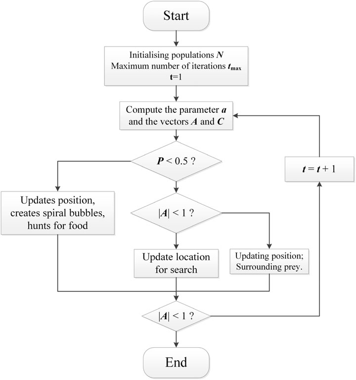
Figure 1. Flowchart of the WOA algorithm.

2.3 SHAP

SHAP is a method rooted in the Shapley value theory from game theory, aimed at providing interpretability for the prediction outcomes of ML models. Originally proposed by Lundberg and Lee (2017) in 2017. Its core idea is to decompose the model’s prediction result into the specific contributions of individual input features, thereby quantifying the impact of each feature on the prediction outcome. The theoretical foundation of SHAP lies in the Shapley value, which calculates the marginal contribution of each player across all possible coalition combinations and determines their fair share through a weighted average approach, achieving equitable distribution. The computational formula for the Shapley value is as Equation 20:

${\varphi }_i={\displaystyle \sum _{S\subseteq N\left\{i\right\}}}\frac{\left|S\right|!\left(n-1-\left|S\right|\right)!}{n!}\left[f_x\left(S\cup \left\{i\right\}\right)-f_x\left(S\right)\right](20)$

where ${\varphi }_i$ denotes the contribution of the ith eigenvalue, N represents the set of all features, Sdenotes a subset of the given predictive features, $f_x\left(S\cup \left\{i\right\}\right)$ denotes the result of the model containing the ith feature, $f_x\left(S\right)$ denotes the result of the model without the ith feature. Finally, SHAP generates an interpretable model through additive feature imputation, which is defined as a linear summation of the input variables.

3 Dataset

3.1 Description of the data

Based on existing research findings, this study integrates a total of 305 sample data points sourced from nine different countries (China, India, Nepal, Venezuela, Austria, Greece, Bhutan, Japan, and Turkey), constructing a novel dataset. (Bo et al., 2023; Feng and Jimenez, 2015; Jimenez and Recio, 2011). Within this dataset, squeezing cases constitute the majority, totaling 235 samples, while non-squeezing cases account for 70 samples. Table 1 provides a detailed overview of the statistical characteristics of the dataset.

Table 1

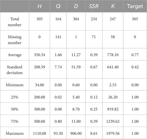
Table 1. Statistical characteristics of features.

The database encompasses five key parameters that influence tunnel squeezing (Aydan et al., 1993; Goel et al., 1995; Hoek and Marinos, 2000). Including tunnel burial depth (H), tunnel diameter (D), support stiffness (K), rock excavation quality index (Q), and strength-to-stress ratio (SSR). The calculation of These parameters are expressed as equations, as listed in Table 2.

Table 2

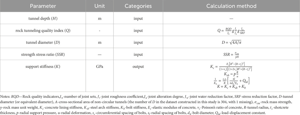
Table 2. Feature description.

Tunnel burial depth (H): The depth of a tunnel significantly influences the stress state of its surrounding strata. As depth increases, geo-stresses, particularly vertical stresses, gradually intensify, potentially leading to higher compression deformation in the tunnel’s surrounding rock. Consequently, tunnel depth is a crucial factor that must be considered when assessing the risk of squeezing.

Tunnel diameter (D): The diameter of a tunnel directly determines the volume of rock to be removed during excavation and the exposed area of surrounding rock post-excavation, making it a vital parameter in assessing the likelihood of squeezing phenomena. A larger tunnel diameter implies greater excavation disturbance and a larger exposed area of surrounding rock, thereby elevating the risks of rock instability and compression deformation.

Support stiffness (K): The stiffness of support structures (such as linings and rockbolts) plays a crucial role in the stability of tunnel surrounding rock and is key to controlling tunnel squeezing deformation. Appropriate support stiffness can effectively resist the squeezing deformation of surrounding rock, maintaining the shape and dimensions of the tunnel. However, excessively high support stiffness may lead to an overly intense interaction between the support structures and surrounding rock, potentially exacerbating squeezing phenomena.

Rock excavation quality index (Q): The Q-value, an index comprehensively reflecting the drill ability and integrity of rock, is widely used in the classification of surrounding rock in tunnel engineering. A higher Q-value indicates harder and more intact rock, which possesses greater resistance to squeezing. Consequently, the Q-value serves as an important reference for assessing the risk of squeezing in tunnel surrounding rock.

Strength-to-stress ratio (SSR): SSR refers to the ratio of the uniaxial compressive strength of rock to the maximum principal stress, reflecting the resistance of rock to failure under geo-stress. A lower SSR indicates relatively lower rock strength, rendering it prone to damage and squeezing deformation under higher geo-stresses. Therefore, SSR is a critical parameter for assessing the stability of tunnel surrounding rock and the risk of squeezing.

It should be noted that, due to the high costs and risks associated with underground engineering, collecting complete tunnel data is challenging, and some samples in the database have one or more missing values. As illustrated in Figure 2, the number of missing values of Q, D, SSR and K are 141, 1, 71 and 58, respectively. In this research, the sample data were collected from engineering cases and relevant literature, and the absence of data is unrelated to the values of other features. In other words, the data missing mechanism in the dataset is characterized as Missing Completely at Random (MCAR).

Figure 2

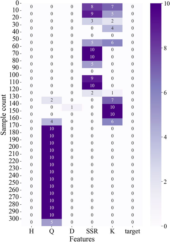
Figure 2. Distribution of missing values in the database.

3.2 Data imputation

The impact of missing training sample data on model prediction performance is multifaceted, particularly in classification problems. When the class labels for certain observations are missing, the model fails to correctly learn the features and class information of these samples during training, leading to prediction results that may be biased towards other existing classes. This decreases the overall prediction accuracy and subsequently reduces the model’s generalization ability. Commonly used methods for handling incomplete datasets include missing value imputation and deletion of missing samples. Performing a simple deletion of missing data in a dataset can lead to the loss of valuable information contained within the missing samples. Considering the widely adoption of KNN algorithm in imputation tasks (An et al., 2024; Bo et al., 2023), it is employed in this study to fill in the missing data, thereby preserving the valid information within the absent samples.

3.3 Synthetic Minority Oversampling Technique (SMOTE)

In the domain of data science and ML, the problem of class imbalance is a prevalent challenge that significantly impacts the performance and generalization ability of classification models. To effectively address this issue, Nitesh Chawla et al. proposed the Synthetic Minority Over-sampling Technique (SMOTE) in 2002. This technique balances the dataset by synthetically generating new minority class samples, thereby enhancing the model’s ability to recognize the minority class. The SMOTE algorithm represents a significant improvement over traditional random over-sampling methods, which simply duplicate minority class samples to increase their quantity. However, this approach can lead to overfitting as the training set contains a large number of duplicated samples. In contrast, SMOTE increases the diversity of the dataset by synthesizing new, diverse minority class samples, thereby avoiding the issue of overfitting. The SMOTE algorithm randomly selects a minority class sample as the base sample. In the feature space, using Euclidean distance as the metric, it calculates the distance from this base sample to all minority class samples and identifies its k nearest neighbors. For each base sample, based on its k nearest neighbors, SMOTE randomly selects one or more of these neighbor samples. It then randomly selects a point along the line segment connecting these two samples to serve as the newly synthesized sample. Specifically, the formula for generating a new sample is as shown in Equation 21:

$NewSample=MinoritySample+\lambda \times \left(NeighborSample-MinoritySample\right)(21)$

where λ is a random number between 0 and 1, used for random interpolation along the line segment connecting the base sample and the neighbor sample. Depending on the degree of data imbalance and the preset sampling ratio, the above steps are repeated until a sufficient number of minority class samples are synthesized to achieve data balance. The primary advantage of the SMOTE algorithm lies in its ability to generate new, diverse minority class samples, effectively mitigating the class imbalance problem and enhancing the performance of classification models. Furthermore, by synthesizing samples, the model is able to learn more about the feature combinations of the minority class, strengthening its generalization ability.

4 Tunnel squeezing prediction model

This paper constructs 6 ML models and compares their performance in predicting tunnel squeezing, aiming to identify the best-performing model for accurately predicting tunnel squeezing and providing reference and guidance for safe tunnel construction and timely decision-making. The process of ML model construction and performance analysis is illustrated in Figure 3. This study primarily encompasses three stages: data preprocessing, model training and testing, result analysis, and model interpretation. Specifically, the first stage involves preprocessing the collected data, establishing the feature system, filling missing data, addressing class imbalance issue in the database using SMOTE, and feature system update. The second stage involves constructing 6 ML models for training and testing, with model optimization performed using the WOA. In the third stage, the prediction results of the 6 ML models are analyzed to determine the best-performing model, and the SHAP is employed for model explanation.

Figure 3

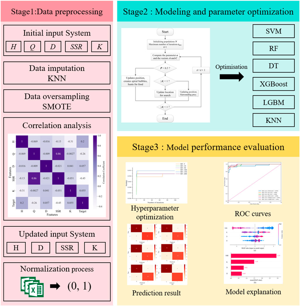
Figure 3. Flowchart for predicting tunnel squeezing using ML.

4.1 Data preprocessing

In this study, five parameters including H, Q, D, SSR, and K were initially selected to construct the dataset for training the ML models. The missing data in the dataset was imputed using KNN, and the SMOTE was applied for data over-sampling to address the issue of class imbalance (Dablain et al., 2023; Fernández et al., 2018; Fix and Hodges, 1989; Mahdevari et al., 2012). In the KNN imputation process, the parameter K was set to be 15, and in the SMOTE over-sampling process, the parameter K was also set as 15. After preparing the database, an initial analysis of the database were conducted by calculating the Pearson correlation coefficient of the database. The Pearson correlation coefficient plot serves to visualize the linear correlation between two variables, with values ranging from −1 to 1. A value of −1 indicates a perfect negative correlation, 1 indicates a perfect positive correlation, and 0 indicates no correlation.

In statistical analysis, a correlation coefficient with an absolute value exceeding 0.6 is generally indicative of a strong linear relationship between two variables. As depicted in Figure 4, the correlation coefficient between variables Q and SSR is 0.86, which substantiates a high degree of correlation between them. Conversely, the absolute values of the correlation coefficients for the remaining features are all below 0.45, suggesting that these variables exhibit relatively low intercorrelations. To mitigate data redundancy, which can inflate the computational burden on ML models, it is prudent to eliminate features that demonstrate high correlation. Given that the variable Q has 141 missing values, a higher count than that of SSR, it is deemed appropriate to exclude Q from the set of input features. Consequently, the revised input feature system comprises four variables: H, D, SSR, and K. This streamlined feature set is expected to enhance the efficiency and predictive accuracy of the ML models employed in the analysis. Further, the dataset, post-imputation and over-sampling, underwent standardization. Subsequently, it was randomly split into a training set and a test set at an 8:2 ratio.

Figure 4

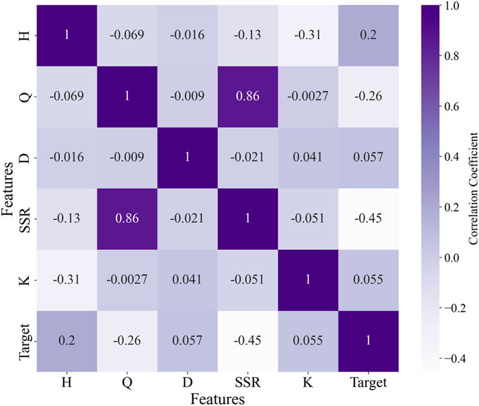
Figure 4. Correlation analysis.

4.2 Model construction and optimization

Six different ML algorithms were employed to construct classification prediction models, and the WOA was utilized to optimize the hyperparameters of these ML models. The whale population sizes were set to 5, 10, 50, 100, 150, and 200, respectively, with 100 iterations for each optimization process. To avoid overfitting, 5-fold cross-validation was adopted on the training set during the optimization. Figure 5 illustrates the optimization curves of the 6 ML models with varying population sizes. As depicted in Figure 5, among the configured population sizes, the optimal population sizes for maximizing the average 5-fold cross-validation accuracy on the training set were 10, 50, 10, 50, 200, and 150, respectively, for SVM, RF, DT, XGBoost, LGBM, and KNN. The corresponding average accuracies achieved were 93.55%, 95.94%, 95.78%, 97.87%, 97.87%, and 93.61%. Therefore, to achieve optimal hyperparameter optimization using the WOA for SVM, RF, DT, XGBoost, LGBM, and KNN models, the population sizes should be set to 10, 50, 10, 50, 200, and 150, respectively. The optimized hyperparameters resulting from this process are presented in Table 3 and the corresponding WOA parameters that yielded the optimal hyperparameters are listed in Table 4.

Figure 5

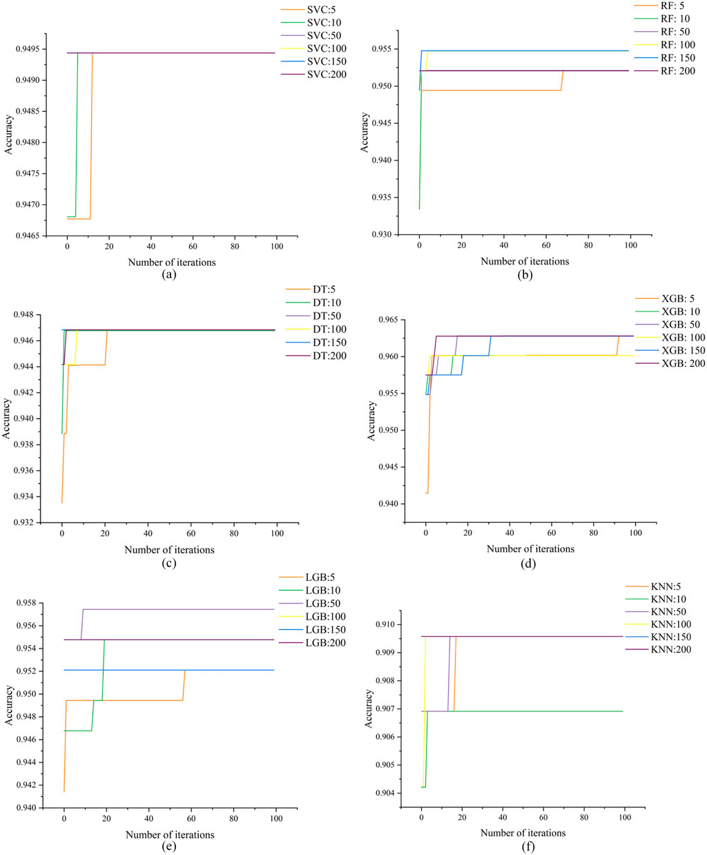
Figure 5. Prediction results of six models on the test set: (A) SVM; (B) RF; (C) DT; (D) XGBoost; (E) LGBM; (F) KNN.

Table 3

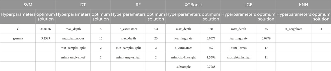
Table 3. Results of hyper-parameter optimization of WOA model.

Table 4

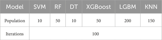
Table 4. The WOA parameters achieving the best hyperparameters of the 6 ML models.

4.3 Analysis of prediction results

To comprehensively evaluate and compare the predictive performance of various ML models, this study conducted a comparative analysis of the prediction performance of the SVM, RF, DT, XGBoost, LGBM, and KNN models optimized by the WOA on the test set. This was done to validate and compare the predictive capabilities of each model.

Confusion matrix, also known as an error matrix or contingency table, is a widely utilized visualization tool in ML, particularly in the realm of supervised learning. In the context of evaluating image accuracy, the confusion matrix plays a pivotal role. It primarily serves to compare the discrepancies between the output results of a classification algorithm and the actual observed values. By presenting the classification accuracy in an intuitive and structured matrix format, the confusion matrix accurately showcases the precision of the classification outcomes. The specific form of a confusion matrix is outlined in Table 5 as follows:

Table 5

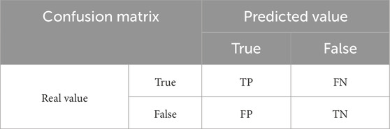
Table 5. Confusion matrix parameter significance.

Specifically, True Positives (TP) refer to instances that are correctly predicted as belonging to the positive class and indeed are positive. True Negatives (TN) involve instances that are predicted to belong to the negative class and indeed are negative. False Positives (FP) occur when instances are incorrectly predicted as belonging to the positive class, whereas they are actually negative. Lastly, False Negatives (FN) arise when instances are predicted to belong to the negative class, but they are actually positive. The calculation of the four index is shown in Table 6.

Table 6

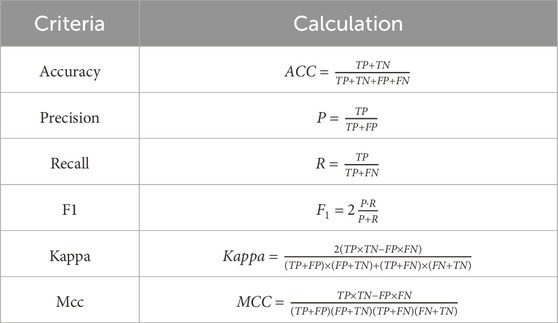
Table 6. Model performance prediction metrics.

The prediction results of the six machine learning models on the test set are illustrated in Figure 6. For the 54 non-squeezing samples, the SVM model made four prediction error among the non-squeezing samples, while the KNN model and DT each made 2 prediction errors. The RF model and LGBM model yielded 1 prediction error each, and both the XGBoost model accurately predicted all the non-squeezing samples in the test set. On the other hand, for the 41 squeezing samples, all models incurred 3 prediction errors each. In summary, the XGBoost model demonstrated the highest prediction accuracy on the test set.

Figure 6

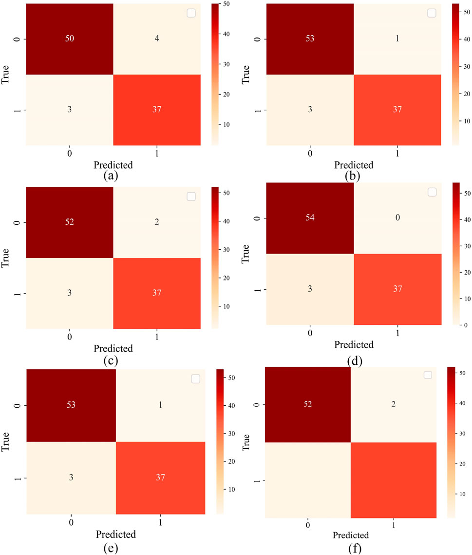
Figure 6. Prediction results of six models on the test set: (A) SVM; (B) RF; (C) DT; (D) XGBoost; (E) LGBM; (F) KNN (1 indicates squeezing and 0 indicates non-squeezing).

The comprehensive prediction performance of the six models established in this study on the test set is presented in Table 7. The prediction accuracies of the SVM, RF, DT, XGBoost, LGBM, and KNN models on the test set are 0.9255, 0.9574, 0.9468, 0.9681, 0.9574, and 0.9468, respectively. The cumulative values of the six performance indicators are 5.3631, 5.6305, 5.5391, 5.7243, 5.6305, and 5.5391, respectively. The WOA-XGBoost model exhibited the highest prediction accuracy, closely followed by LGBM and RF. The ranking of the prediction performance among the 6 ML models is XGBoost > LGBM = RF > KNN = DT > SVM.

Table 7

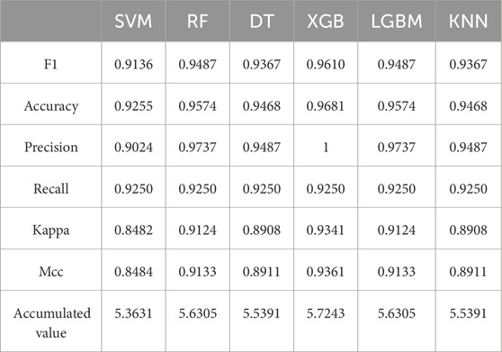
Table 7. Comprehensive performance table for ML model prediction.

The ROC curve is plotted with the False Positive Rate (FPR) on the x-axis and the True Positive Rate (TPR, also known as the sensitivity or recall) on the y-axis. An ideal classifier would be located at the top-left corner of the ROC space (TPR=1, FPR=0), while a classifier that performs at the level of random guessing would follow the diagonal line. The Area Under the Curve (AUC) of the ROC curve is a crucial metric for evaluating the overall performance of a model, with higher AUC values indicating stronger ability to distinguish between positive and negative classes. The ROC curves of the 4 ML models are shown in Figure 7. Among the six models, the ROC curve of the WOA-XGBoost model is the closest to the top-left corner of the ROC space, with an AUC of 0.993, which is higher than the AUCs of the other five models. This suggests that the WOA-XGBoost model exhibits superior prediction performance on the test set compared to the other five models.

Figure 7

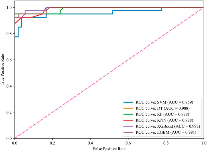
Figure 7. ROC curve of ML model on the test set.

4.4 Comparative analysis with related studies

The ML performance of related studies is summarized in Table 8. The accuracy is taken as the standard for comparison. The WOA-XGBoost model established in this study demonstrates higher accuracy compared to most of the related studies, indicating that the WOA-XGBoost model is as reliable as the ML models in the previous studies.

Table 8

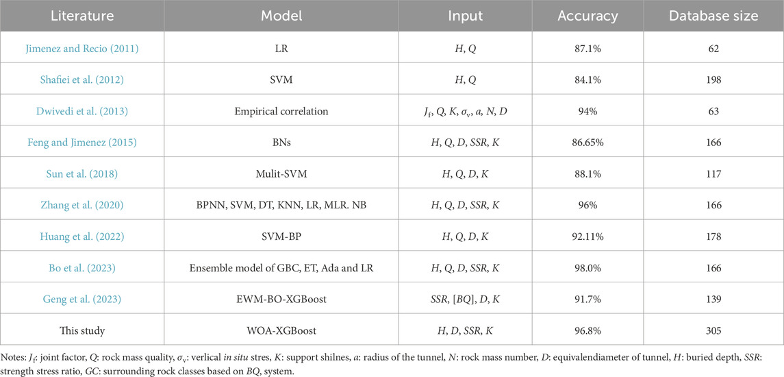
Table 8. Summary of tunnel squeezing prediction performance of related studies.

4.5 Model interpretation

With the profound application of ML technologies across numerous domains, the complexity and opacity (or black-box nature) of these models have become increasingly prominent. While this inherent complexity significantly enhances predictive accuracy, the intricate nonlinear relationships between model inputs and outputs pose a significant challenge for researchers. To enhance the comprehensibility and trustworthiness of these models, conducting detailed explainability analyses becomes crucial. In this study, we specifically adopted the SHAP framework to conduct a global interpretability analysis of the WOA-XGBoost model, which exhibited the most outstanding performance among the six evaluated models.

Figure 8A illustrates the SHAP values for each data sample and their impact on the model’s output. Red dots represent features of the sample that have a positive contribution to the prediction result, indicating that an increase in the value of that feature would enhance the model’s predicted output. Conversely, blue dots signify features that have a negative contribution to the prediction, meaning that an increase in their values would decrease the model’s predicted output. Variables with higher average SHAP values exert a relatively greater influence on the model’s prediction results. Figure 8B demonstrates that in the WOA-XGBoost model, the SSR feature contributes most significantly to the model’s prediction performance, with an average SHAP value of +2.93. This value significantly surpasses the average SHAP values of features K, D, and H (+1.49, +0.82, +0.69). The ranking of the average SHAP values of the input features clearly indicates the priority relationship of SSR > K > D > H. It is important to note that the current conclusions are based on a specific experimental setup, namely the WOA-XGBoost model prediction analysis with the optimal hyperparameters. Considering SSR contributes the most to the output of the XGBoost model, Figure 9 illustrates the interactions between other input features and their potential impact on the prediction results of the XGBoost model. Given that the performance of ML models and the assessment of input feature importance are highly dependent on model configurations, dataset characteristics, the generalizability of this feature contribution ranking should be approached with caution. Therefore, while the findings of this study are insightful, they should not be absolutized as a universal rule for feature importance across all prediction scenarios.

Figure 8

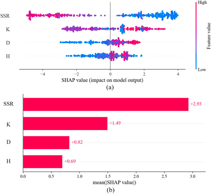
Figure 8. Interpretation results of WOA-XGBoost model: (A) SHAP value; (B) Mean SHAP value.

Figure 9

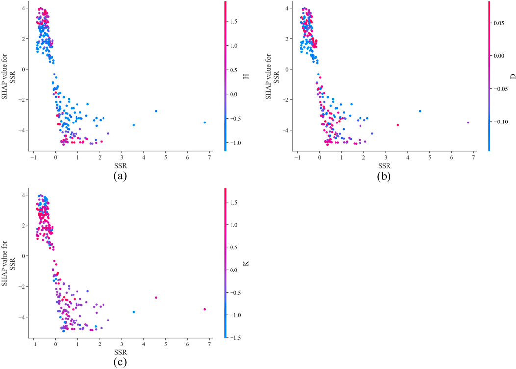
Figure 9. Interaction analysis of SSR and the other input features: (A) Interaction between SSR and H; (B) Interaction between SSR and D; (C) Interactions between SSR and K.

5 Engineering application

5.1 Engineering background

The Huzhu Beishan Extra-Long Tunnel, located in Qinghai Province, China, has a total length of 11,160 m. It traverses a high-altitude and complexly varied terrain with an elevation ranging from 2,815 m to 3,699 m, and the relative elevation difference within the area is as high as 884 m. Additionally, the maximum burial depth of the tunnel is approximately 769 m, posing significant challenges to the stability design, construction difficulty, and safety control of the tunnel project. Due to geological tectonic processes, faulted and fractured zones exist within the tunnel site, as shown in Figure 10. The rock mass in these zones is of extremely poor quality, prone to disasters such as collapses, water intrusions, and large deformations. Figure 11 shows the onsite tunnel works. Therefore, during the tunnel excavation and construction process, ML methods were employed to predict the squeezing probability of the tunnel, ensuring the safety of tunnel construction.

Figure 10

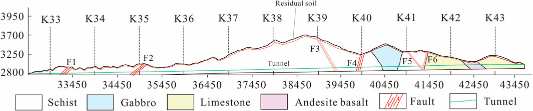
Figure 10. Location of target tunnel.

Figure 11

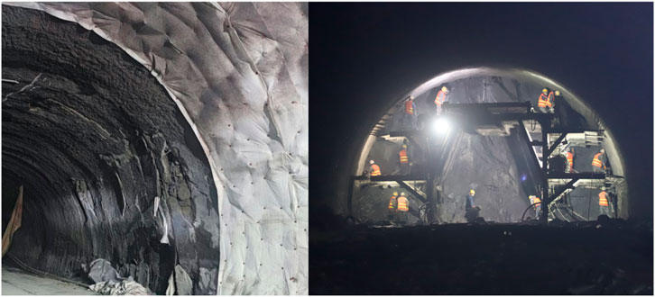
Figure 11. Photographs of onsite tunnel works.

5.2 Squeezing prediction

In this study, the WOA-XGBoost model, which demonstrated the best predictive performance, was utilized to forecast the occurrence of squeezing in ten cross-sections of the tunnel’s right line, including K34+157, K34+160, K35+300, K35+380, K37+180, K38+480, K39+250, K40+480, K40+500, and K40+520. While the values of H and D were obtained from the tunnel design data, the missing values for SSR, and K were imputed using KNN interpolation. The prediction results are presented in Table 9. The probability of squeezing are yielded by the ML model using the function “predict.proba ()”.

Table 9

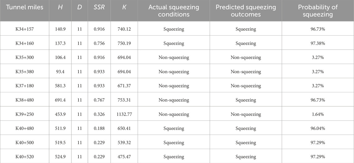
Table 9. Predicting results of tunnel squeezing in HUZHU north mountain engineering.

Based on the prediction results, six sections of the tunnel’s right line, including K34+157, K34+160, K40+480, K38+480, K40+500, and K40+520, were predicted to experience squeezing, with respective probabilities of 96.73%, 97.38%, 96.73%, 96.04%, 91.29%, and 91.29%. The remaining four sections (K35+300, K35+380, K37+180, K39+250) are predicted to be non-squeezing, with respective probabilities of 3.27%, 3.27%, 3.27%, and 1.64%. It can be observed that, except for the prediction results of the K38+480 section which do not match the actual results, the prediction results of the other sections are consistent with the actual squeezing conditions. This indicates that the constructed WOA-XGBoost model possesses high reliability in the task of predicting squeezing in actual tunnel engineering.

6 Conclusion

This study constructed six different ML models for tunnel squeezing prediction and optimized their hyperparameters using the WOA, resulting in WOA-SVM, WOA-RF, WOA-DT, WOA-XGB, WOA-LGBM, and WOA-KNN. To address the presence of missing values in the dataset, data imputation and oversampling techniques were implemented to enhance the quality of the dataset and facilitate accurate predictions by the models. Subsequently, the most prominent model, WOA-XGBoost, was analyzed in depth using the SHAP framework. The core input features of this model encompassed critical parameters such as H, D, SSR, and K. To comprehensively evaluate the predictive performance of the models, six performance metrics, including ACC, F1 Score, Kappa, and MCC, were employed. Furthermore, the optimized WOA-XGBoost model was applied to 10 distinct tunnel section squeezing prediction tasks to validate its applicability and accuracy in tunnel engineering. The following conclusions were drawn from this study:

(1) Among the WOA-SVM, WOA-RF, WOA-DT, WOA-XGB, WOA-LGBM, and WOA-KNN models, the prediction accuracies on the test set were 0.9255, 0.9574, 0.9468, 0.9681, 0.9574, and 0.9468, respectively. The cumulative values of the prediction performance evaluation metrics were 5.3631, 5.6305, 5.5391, 5.7243, 5.6305, and 5.5391, respectively. The WOA-XGBoost model demonstrated superior prediction accuracy and cumulative performance evaluation metrics compared to the other five models, exhibiting the best predictive performance.

(2) The SHAP explanation results revealed that the average SHAP values for SSR, K, D, and H were 2.93, 1.49, 0.82, and 0.69, respectively. Among the four input features, SSR had the highest importance in influencing the model’s output, with the order of importance being SSR > K >D > H.

(3) Ten representative tunnel sections from the Hubei Beishan Tunnel were selected for tunnel squeezing prediction. Except for the prediction results of the K38+480 section which did not match the actual results, the prediction results of the other sections were consistent with the actual squeezing conditions.

This study achieved tunnel squeezing prediction based on an imbalanced and missing dataset. However, there are still limitations that need further investigation. Firstly, the binary classification strategy adopted in this study is not fine enough and has thereby limited effective guidance for engineering applications. Future research will consider constructing multi-class classification models to provide a more detailed classification of tunnel squeezing degrees, thereby enhancing its guiding role in tunnel engineering. Secondly, the data sample size and range are limited still, and future work might collect more samples to expand the dataset to further improve the applicability and generalization performance of the models.

Data availability statement

The raw data supporting the conclusions of this article will be made available by the authors, without undue reservation.

Author contributions

PG: Funding acquisition, Project administration, Resources, Writing–original draft, Writing–review and editing, Conceptualization, Data curation, Investigation, Methodology. GO: Resources, Supervision, Writing–review and editing, Conceptualization, Validation, Project administration. FL: Formal Analysis, Investigation, Software, Writing–original draft, Validation, Visualization. WL: Investigation, Validation, Writing–original draft, Data curation, Methodology, Visualization. QW: Investigation, Writing–original draft, Data curation, Formal Analysis, Visualization. CP: Writing–original draft, Data curation, Investigation, Visualization. XC: Investigation, Writing–original draft, Data curation, Formal Analysis, Visualization.

Funding

The author(s) declare that financial support was received for the research, authorship, and/or publication of this article. This study was financially supported by National Natural Science Foundation of China (52008383), Natural Science Foundation of Hubei Province (2023AFB369).

Conflict of interest

Authors FL, WL, QW, and CP were employed by Xinjiang Water Conservancy Development and Construction Group Co., Ltd.

The remaining authors declare that the research was conducted in the absence of any commercial or financial relationships that could be construed as a potential conflict of interest.

Generative AI statement

The author(s) declare that no Generative AI was used in the creation of this manuscript.

Publisher’s note

All claims expressed in this article are solely those of the authors and do not necessarily represent those of their affiliated organizations, or those of the publisher, the editors and the reviewers. Any product that may be evaluated in this article, or claim that may be made by its manufacturer, is not guaranteed or endorsed by the publisher.

References

An, X., Zheng, F., Jiao, Y., Li, Z., Zhang, Y., and He, L. (2024). Optimized machine learning models for predicting crown convergence of plateau mountain tunnels. Transp. Geotech. 46, 101254. doi:10.1016/j.trgeo.2024.101254

CrossRef Full Text | Google Scholar

Aristiawati, K., Siswantining, T., Sarwinda, D., and Soemartojo, S. M. (2019). Missing values imputation based on fuzzy C-Means algorithm for classification of chronic obstructive pulmonary disease (COPD). AIP Conf. Proc. 2192 (1), 060003. doi:10.1063/1.5139149

CrossRef Full Text | Google Scholar

Aydan, Ö., Akagi, T., and Kawamoto, T. (1993). The squeezing potential of rocks around tunnels; Theory and prediction. Rock Mech. Rock Eng. 26 (2), 137–163. doi:10.1007/BF01023620

CrossRef Full Text | Google Scholar

Beretta, L., and Santaniello, A. (2016). Nearest neighbor imputation algorithms: a critical evaluation. BMC Med. Inf. Decis. Mak. 16 (3), 74. doi:10.1186/s12911-016-0318-z

PubMed Abstract | CrossRef Full Text | Google Scholar

Bo, Y., Huang, X., Pan, Y., Feng, Y., Deng, P., Gao, F., et al. (2023). Robust model for tunnel squeezing using Bayesian optimized classifiers with partially missing database. Undergr. Space 10, 91–117. doi:10.1016/j.undsp.2022.11.001

CrossRef Full Text | Google Scholar

Chen, H., Li, X., Feng, Z., Wang, L., Qin, Y., Skibniewski, M. J., et al. (2023). Shield attitude prediction based on Bayesian-LGBM machine learning. Inf. Sci. 632, 105–129. doi:10.1016/j.ins.2023.03.004

CrossRef Full Text | Google Scholar

Chen, T., and Guestrin, C. (2016). XGBoost: a scalable tree boosting system. Proc. 22nd ACM SIGKDD Int. Conf. Knowl. Discov. Data Min., 785–794. doi:10.1145/2939672.2939785

CrossRef Full Text | Google Scholar

Chen, Y., Li, T., Zeng, P., Ma, J., Patelli, E., and Edwards, B. (2020). Dynamic and probabilistic multi-class prediction of tunnel squeezing intensity. Rock Mech. Rock Eng. 53 (8), 3521–3542. doi:10.1007/s00603-020-02138-8

CrossRef Full Text | Google Scholar

Dablain, D., Krawczyk, B., and Chawla, N. V. (2023). DeepSMOTE: fusing deep learning and SMOTE for imbalanced data. IEEE Trans. Neural Netw. Learn. Syst. 34 (9), 6390–6404. doi:10.1109/TNNLS.2021.3136503

PubMed Abstract | CrossRef Full Text | Google Scholar

Dong, W., Huang, Y., Lehane, B., and Ma, G. (2020). XGBoost algorithm-based prediction of concrete electrical resistivity for structural health monitoring. Automation Constr. 114, 103155. doi:10.1016/j.autcon.2020.103155

CrossRef Full Text | Google Scholar

Dwivedi, R. D., Singh, M., Viladkar, M. N., and Goel, R. K. (2013). Prediction of tunnel deformation in squeezing grounds. Eng. Geol. 161, 55–64. doi:10.1016/j.enggeo.2013.04.005

CrossRef Full Text | Google Scholar

Fathipour-Azar, H. (2022). Multi-level machine learning-driven tunnel squeezing prediction: review and new insights. Archives Comput. Methods Eng. 29 (7), 5493–5509. doi:10.1007/s11831-022-09774-z

CrossRef Full Text | Google Scholar

Feng, X., and Jimenez, R. (2015). Predicting tunnel squeezing with incomplete data using Bayesian networks. Eng. Geol. 195, 214–224. doi:10.1016/j.enggeo.2015.06.017

CrossRef Full Text | Google Scholar

Fernández, A., García, S., Herrera, F., and Chawla, N. V. (2018). SMOTE for learning from imbalanced data: progress and challenges, marking the 15-year anniversary. J. Artif. Int. Res. 61 (1), 863–905. doi:10.1613/jair.1.11192

CrossRef Full Text | Google Scholar

Fix, E., and Hodges, J. L. (1989). Discriminatory analysis. Nonparametric discrimination: consistency properties. Int. Stat. Review/Rev. Int. Stat. 57 (3), 238–247. doi:10.2307/1403797

CrossRef Full Text | Google Scholar

Geng, X., Wu, S., Zhang, Y., Sun, J., Cheng, H., Zhang, Z., et al. (2023). Developing hybrid XGBoost model integrated with entropy weight and Bayesian optimization for predicting tunnel squeezing intensity. Nat. Hazards Q3, 751–771. doi:10.1007/s11069-023-06137-0

CrossRef Full Text | Google Scholar

Ghiasi, V., Ghiasi, S., and Prasad, A. (2012). Evaluation of tunnels under squeezing rock condition. J. Eng. Des. Technol. 10 (2), 168–179. doi:10.1108/17260531211241167

CrossRef Full Text | Google Scholar

Goel, R. K., Jethwa, J. L., and Paithankar, A. G. (1995). Tunnelling through the young Himalayas—a case history of the Maneri-Uttarkashi power tunnel. Eng. Geol. 39 (1), 31–44. doi:10.1016/0013-7952(94)00002-J

CrossRef Full Text | Google Scholar

Guo, D., Song, Z., Liu, N., Xu, T., Wang, X., Zhang, Y., et al. (2024). Performance study of hard rock cantilever roadheader based on PCA and DBN. Rock Mech. Rock Eng. 57 (4), 2605–2623. doi:10.1007/s00603-023-03698-1

CrossRef Full Text | Google Scholar

Hoek, E. (2001). Big tunnels in bad rock. J. Geotechnical Geoenvironmental Eng. 127 (9), 726–740. doi:10.1061/(ASCE)1090-0241(2001)127:9(726)

CrossRef Full Text | Google Scholar

Hoek, E., and Marinos, P. (2000). Predicting tunnel squeezing problems in weak heterogeneous rock masses. Tunn. and Tunnell. Inter. 2, 1–21.

Google Scholar

Huang, H., Wang, C., Zhou, M., and Qu, L. (2024). Compressive strength detection of tunnel lining using hyperspectral images and machine learning. Tunn. Undergr. Space Technol. 153, 105979. doi:10.1016/j.tust.2024.105979

CrossRef Full Text | Google Scholar

Huang, J., Mao, B., Bai, Y., Zhang, T., and Miao, C. (2020). An integrated fuzzy C-means method for missing data imputation using taxi GPS data. Sensors 20 (7), 1992. doi:10.3390/s20071992

PubMed Abstract | CrossRef Full Text | Google Scholar

Huang, Z., Liao, M., Zhang, H., Zhang, J., Ma, S., and Zhu, Q. (2022). Predicting tunnel squeezing using the svm-bp combination model. Geotech. Geol. Eng. 40 (3), 1387–1405. doi:10.1007/s10706-021-01970-1

CrossRef Full Text | Google Scholar

Jain, A., and Rao, K. S. (2022). Empirical correlations for prediction of tunnel deformation in squeezing ground condition. Tunn. Undergr. Space Technol. 125, 104501. doi:10.1016/j.tust.2022.104501

CrossRef Full Text | Google Scholar

Jimenez, R., and Recio, D. (2011). A linear classifier for probabilistic prediction of squeezing conditions in Himalayan tunnels. Eng. Geol. 121 (3), 101–109. doi:10.1016/j.enggeo.2011.05.006

CrossRef Full Text | Google Scholar

Li, C., and Mei, X. (2023). Application of SVR models built with AOA and Chaos mapping for predicting tunnel crown displacement induced by blasting excavation. Appl. Soft Comput. 147, 110808. doi:10.1016/j.asoc.2023.110808

CrossRef Full Text | Google Scholar

Li, K., Zhang, Z., Guo, H., Li, W., and Yan, Y. (2023). Prediction method of pipe joint opening-closing deformation of immersed tunnel based on singular spectrum analysis and SSA-SVR. Appl. Ocean Res. 135, 103526. doi:10.1016/j.apor.2023.103526

CrossRef Full Text | Google Scholar

Liang, D., Rui, Z., and Yuguang, F. (2024). A robust evaluating strategy of tunnel deterioration using ensemble machine learning algorithms. Eng. Appl. Artif. Intell. 133, 108364. doi:10.1016/j.engappai.2024.108364

CrossRef Full Text | Google Scholar

Lundberg, S., and Lee, S.-I. (2017). A unified approach to interpreting model predictions. arXiv. arXiv:1705.07874. doi:10.48550/arXiv.1705.07874

CrossRef Full Text | Google Scholar

Mahdevari, S., Torabi, S. R., and Monjezi, M. (2012). Application of artificial intelligence algorithms in predicting tunnel convergence to avoid TBM jamming phenomenon. Int. J. Rock Mech. Min. Sci. 55, 33–44. doi:10.1016/j.ijrmms.2012.06.005

CrossRef Full Text | Google Scholar

Martin, C. D., Kaiser, P. K., and McCreath, D. R. (2011). Hoek-Brown parameters for predicting the depth of brittle failure around tunnels. Can. Geotechnical J. 36, 136–151. doi:10.1139/t98-072

CrossRef Full Text | Google Scholar

Mikaeil, R., Shaffiee Haghshenas, S., and Sedaghati, Z. (2019). Geotechnical risk evaluation of tunneling projects using optimization techniques (case study: the second part of Emamzade Hashem tunnel). Nat. Hazards 97 (3), 1099–1113. doi:10.1007/s11069-019-03688-z

CrossRef Full Text | Google Scholar

Mirjalili, S., and Lewis, A. (2016). The whale optimization algorithm. Adv. Eng. Softw. 95, 51–67. doi:10.1016/j.advengsoft.2016.01.008

CrossRef Full Text | Google Scholar

Panthi, K. K. (2013). Predicting tunnel squeezing: a discussion based on two tunnel projects. Hydro Nepal J. Water, Energy Environ. 12, 20–25. doi:10.3126/hn.v12i0.9027

CrossRef Full Text | Google Scholar

Shafiei, A., Parsaei, H., and Dusseault, M. B. (2012). “Rock Squeezing prediction by a support vector machine classifier” in U.S. Rock Mechanics/Geomechanics Symposium. Available at: https://dx.doi.org/.

Google Scholar

Singh, B., Jethwa, J. L., Dube, A. K., and Singh, B. (1992). Correlation between observed support pressure and rock mass quality. Tunn. Undergr. Space Technol. 7 (1), 59–74. doi:10.1016/0886-7798(92)90114-W

CrossRef Full Text | Google Scholar

Singh, M., Singh, B., and Choudhari, J. (2007). Critical strain and squeezing of rock mass in tunnels. Tunn. Undergr. Space Technol. 22 (3), 343–350. doi:10.1016/j.tust.2006.06.005

CrossRef Full Text | Google Scholar

Sun, Y., Feng, X., and Yang, L. (2018). Predicting tunnel squeezing using multiclass support vector machines. Adv. Civil Eng. 2018 (1), 4543984. doi:10.1155/2018/4543984

CrossRef Full Text | Google Scholar

Wang, K., Zhang, Z., Wu, X., and Zhang, L. (2022). Multi-class object detection in tunnels from 3D point clouds: an auto-optimized lazy learning approach. Adv. Eng. Inf. 52, 101543. doi:10.1016/j.aei.2022.101543

CrossRef Full Text | Google Scholar

Wang, M., Ye, X.-W., Ying, X.-H., Jia, J.-D., Ding, Y., Zhang, D., et al. (2024). Data imputation of soil pressure on shield tunnel lining based on random forest model. Sensors 24 (5), 1560. doi:10.3390/s24051560

PubMed Abstract | CrossRef Full Text | Google Scholar

Ye, X.-W., Jin, T., and Chen, Y.-M. (2022). Machine learning-based forecasting of soil settlement induced by shield tunneling construction. Tunn. Undergr. Space Technol. 124, 104452. doi:10.1016/j.tust.2022.104452

CrossRef Full Text | Google Scholar

Zhang, J., Li, D., and Wang, Y. (2020). Predicting tunnel squeezing using a hybrid classifier ensemble with incomplete data. Bull. Eng. Geol. Environ. 79 (6), 3245–3256. doi:10.1007/s10064-020-01747-5

CrossRef Full Text | Google Scholar

Zhao, D., He, Y., Chen, X., Wang, J., Liu, Y., Zhang, Q., et al. (2024). Data-driven intelligent prediction of TBM surrounding rock and personalized evaluation of disaster-inducing factors. Tunn. Undergr. SPACE Technol. 148, 105768. doi:10.1016/j.tust.2024.105768

CrossRef Full Text | Google Scholar

Zhou, X., Zhao, C., and Bian, X. (2023). Prediction of maximum ground surface settlement induced by shield tunneling using XGBoost algorithm with golden-sine seagull optimization. Comput. Geotechnics 154, 105156. doi:10.1016/j.compgeo.2022.105156

CrossRef Full Text | Google Scholar

Zhu, H., Yan, J., and Liang, W. (2019). Challenges and development prospects of ultra-long and ultra-deep mountain tunnels. Engineering 5 (3), 384–392. doi:10.1016/j.eng.2019.04.009

CrossRef Full Text | Google Scholar