Fast forward modeling and response analysis of extra-deep azimuthal resistivity measurements in complex model

The Extra-Deep Azimuthal Resistivity Measurements (EDARM) tool, as an emerging technology, can effectively identify geological interfaces within a range of several tens of meters around the borehole, providing geological structures for directional drilling, and effectively improving reservoir encounter rates and enhancing oil and gas recovery rates. However, the signal is jointly affected by interfaces located both ahead of the drill bit and around the borehole, making it impossible to directly obtain the interface position from the signal. Considering the increased detection range of EDARM and the requirements for computational efficiency, this paper presents a 2.5-dimensional (2.5D) finite element method (FEM). By leveraging the symmetry of simulated signals in the spectral domain, the algorithm reduces computation time by 50%, significantly enhancing computational efficiency while preserving accuracy. During the geosteering process, fault and wedge models were simulated, and various feature parameters were extracted to assess their impact on the simulation outcomes of EDARM. The results show that both Look-around and Look-ahead modes exhibit sensitivity to changes in the angle of the geological interface. Crossplot analysis allows for effective identification of interface inclinations and the distances between the instrument and the geological interface. This recognition method is quick, intuitive, and yields reliable results.

1 Introduction

Geosteering is a critical technology for minimizing development costs and optimizing the extraction of complex oil and gas resources. It directs the drilling trajectory of instruments in high-angle and horizontal wells (Li et al., 2005; Li et al., 2014; Wu et al., 2020; Omeragic et al., 2005; Bittar and Aki, 2015; Bell et al., 2006). Over the past several decades, geosteering technology has evolved from post-drilling track adjustments to active steering (Bittar et al., 2009; Li et al., 2014; Hu and Fan, 2018; Wang and Fan, 2019). The detection range has expanded from a few meters to several tens of meters, significantly reducing the risks associated with drilling operations and enhancing the overall success rate (Iverson et al., 2004; Dupuis and Denichou, 2015). Currently, oil service companies have developed proprietary extra-deep azimuthal resistivity measurement (EDARM) instruments that effectively detect geological anomalies over distances of several tens of meters and identify interfaces ahead of the drill bit, thereby providing geological guidance on a reservoir scale (Hartman et al., 2014; Li and Zhou, 2017).

The Geosphere, developed by Schlumberger, is the first commercially available EDARM instrument capable of detecting resistivity, anisotropy, interfaces, and dipping angles (Seydoux et al., 2014; Thiel et al., 2018). Recent research has focused on the physical aspects, detection performance, and sensitivity of EDARM (Larsen et al., 2015; Wu et al., 2018; Wang et al., 2019a; Zhang et al., 2021; Wang et al., 2015). Investigations primarily center on its ability to detect interfaces around the instrument within layered media, aiming to ascertain the positional relationship between the instrument and these interfaces (Xia et al., 2019; Wang et al., 2019b; Lu et al., 2019). In specific geological structures, such as fault and wedge models, interfaces may be located ahead of the drill bit. While some researchers have evaluated the Look-ahead capability of the instrument (Constable et al., 2016; Hagiwara, 2018; Lu et al., 2019; Liang et al. 2023), few have explored the relationship between Look-around and Look-ahead modes. Understanding this relationship is essential for accurately determining the distance and angle between the instrument and the interface. Further investigation is needed to elucidate the detection characteristics of EDARM, thereby providing precise and reliable information about adjacent boundaries and formation structures.

The current limitations in the application of EDARM primarily stem from two factors: First, the extended detection range leads to a more complex formation model, which in turn reduces the efficiency of forward modeling; second, the logging response is influenced by interfaces at varying orientations, complicating the inversion process. To address the issue of forward modeling efficiency, the prevalent approach is to apply equivalent dimensionality reduction methods tailored to the characteristics of the while-drilling measurement environment. This involves solving the 3D electromagnetic field using a 2D model, commonly referred to as the 2.5D algorithm. The 2.5D algorithm for while-drilling electromagnetic wave logging was first proposed by Rozas and Pardo in 2016, with a systematic explanation provided in 2018 (Rodríguez-Rozas and Pardo, 2016 and Rodríguez-Rozas et al. 2018). In 2018, Zeng et al. introduced a 2.5D finite difference method (FDM) that simultaneously resolves electric and magnetic field components, enabling more intuitive and implementable modeling of fully anisotropic media. Wu et al. (2019) then applied the 2.5D FDM to logging-while-drilling (LWD), achieving fast and accurate electromagnetic field calculations. Their team later optimized the algorithm with a novel near-optimal quadrature (2022) and Lebedev grid discretization methods (2023) (Wu et al., 2023), reducing the single-point computation time to 7.6 s and further enhancing the 2.5D algorithm’s performance. For EDARM inversion, current efforts have focused on reducing the number of inversion parameters by classifying formation models. Noh et al. (2021) developed a deep learning method to improve inversion efficiency, incorporating a classification module to distinguish between cases with and without fault planes. Wu et al. (2022) used the 2.5D FDM to simulate signal responses under different fault, curved boundary, and unconformity conditions, analyzing variations in the instrument’s maximum detection range. Zhao et al. (2024) applied a coupled physics-driven and data-driven approach to tackle the 2.5D inversion problem, enabling the retrieval of formation parameters under varying dip angles and fault conditions. Overall, while significant progress has been made, further improvements in the computational efficiency of the 2.5D algorithm are necessary, along with a clearer understanding of the response patterns of boundary conditions under different geological scenarios, to fully realize the potential of ultra-deep geosteering.

In this paper, we developed a fast forward algorithm and analyzed the calculation results for various detection modes. The first section discusses the investigation characteristics of the Look-around and Look-ahead modes. In the second section, we propose the 2.5-dimensional finite element method (2.5D FEM) to calculate the responses of complex models. Next, we investigate the detection performance of the Look-around and Look-ahead modes in both fault and wedge models. Additionally, we generated crossplots to determine the vertical distance and angle between the instrument and the interface. Based on the findings from the previous sections, a brief conclusion is presented in the final section.

2 Method

Efficiently and rapidly simulating geological structures, such as faults, folds, and unconformities that frequently occur around the wellbore during drilling, is crucial. Currently, two primary approaches address this issue. One method employs a sliding window processing strategy, treating complex geological structures as equivalent layered models for calculation. However, this approach is suitable only for structurally simple and gradually changing formations and does not guarantee precision (Bakr et al., 2017; Pardo and Torres-Verdín, 2015; Hu et al., 2018). The alternative method utilizes 3D numerical algorithms to simulate geological models in detail, achieving high-precision results (Davydycheva et al., 2003; Jahani et al., 2023; Davydycheva et al., 2023). However, the substantial computational workload and resource consumption lead to reduced computational efficiency, making it inadequate for the real-time demands of logging while drilling.

2.1 Governing equation

In the calculation of electromagnetic wave logging, a magnetic dipole is employed as a source during simulation to address the substantial difference between the spacing and the size of the coils, allowing for the solution of the spatial electromagnetic field. Assuming the time factor is $e^{-iwt}$, in the quasi-steady-state situation, the Maxwell’s equations can be expressed as:

$\nabla \times \mathit{E}-i\omega \mathit{\mu }\mathit{H}=-{\mathit{M}}_i$

$\nabla \times \mathit{H}-\mathit{\sigma }\mathit{E}={\mathit{J}}_i$

where E and H represent electric fields and magnetic fields, the μ and σ represent the magneto conductivity and conductivity, the J_i and M_i represent the current density and the magnetic current density.

The instrument detects signals during the drilling process, remaining unaffected by borehole invasion and mud interference. Typically, the properties of the formation remain stable and unchanged along a certain direction during actual detection, assuming characteristic alignment along the y-axis. To leverage this stability, the spatial Fourier transform can replace solving problems in the 3D spatial domain with a series of 2D spectral domain problems, effectively reducing the dimensionality of the computational model. Based on the frequency domain differential properties of the spatial Fourier transform, the following Equation can be obtained:

$\begin{array}{ll}\hfill \widehat{F}\left[\frac{\mathrm{\partial }f}{\mathrm{\partial }y}\right]& ={\int }_{-\infty }^{\infty }\frac{\mathrm{\partial }f\left(x,y,z\right)}{\mathrm{\partial }y}{e}^{-i{k}_{y}y}dy=i{k}_y{\int }_{-\infty }^{\infty }f\left(x,y,z\right)e^{-i{k}_{y}y}dy\hfill \\ \hfill & =i{k}_y\widehat{F}\left(x,k_y,z\right)\hfill \end{array}$

where $\widehat{F}$ represent the spatial Fourier transform. By using the above equation, we can obtain the expression of the magnetic field in the x and z directions in the spectral domain.

$\begin{array}{l}{\widehat{H}}_x=-\frac{i{k}_y}{{\gamma }_z^2}\frac{\mathrm{\partial }{\widehat{H}}_y}{\mathrm{\partial }x}+\frac{{\sigma }_z}{{\gamma }_z^2}\frac{\mathrm{\partial }{\widehat{E}}_y}{\mathrm{\partial }z}-\frac{{\sigma }_z}{{\gamma }_z^2}{M}_{s,x}\delta \left(A\right)\\ {\widehat{H}}_z=-\frac{i{k}_y}{{\gamma }_x^2}\frac{\mathrm{\partial }{\widehat{H}}_y}{\mathrm{\partial }z}-\frac{{\sigma }_x}{{\gamma }_x^2}\frac{\mathrm{\partial }{\widehat{E}}_y}{\mathrm{\partial }x}-\frac{{\sigma }_x}{{\gamma }_x^2}{M}_{s,z}\delta \left(A\right)\end{array}$

and the electrical field in x and z directions is

$\begin{array}{l}{\widehat{E}}_x=\frac{i\omega {\mu }_0}{{\gamma }_x^2}\frac{\mathrm{\partial }{\widehat{H}}_y}{\mathrm{\partial }z}-\frac{i{k}_y}{{\gamma }_x^2}\frac{\mathrm{\partial }{\widehat{E}}_y}{\mathrm{\partial }x}-\frac{i{k}_y}{{\gamma }_x^2}{M}_{s,z}\delta \left(A\right)\\ {\widehat{E}}_z=-\frac{i\omega {\mu }_0}{{\gamma }_z^2}\frac{\mathrm{\partial }{\widehat{H}}_y}{\mathrm{\partial }x}-\frac{i{k}_y}{{\gamma }_z^2}\frac{\mathrm{\partial }{\widehat{E}}_y}{\mathrm{\partial }z}+\frac{i{k}_y}{{\gamma }_z^2}{M}_{s,x}\delta \left(A\right)\end{array}$

where the ${\widehat{H}}_x$ and ${\stackrel{⌢}{E}}_x$ represent the magnetic field and electrical field in spectral domain, respectively. ${\gamma }_z^2=k_y^2-i\omega {\mu }_0{\sigma }_z$ and ${\gamma }_x^2=k_y^2-i\omega {\mu }_0{\sigma }_x$.

2.2 Grid meshing and resistivity assignment

In finite element algorithms, the accuracy of simulation results is influenced by the density of the discretized mesh. Finer mesh refinement enhances simulation accuracy but results in a significant decline in computational efficiency. Therefore, it is crucial to partition the geological model judiciously. Given that the geological models targeted by multi-component electromagnetic logging exhibit relatively gentle undulations, structured meshes can be utilized within a specific precision range to effectively reduce the size of the solution matrix and enhance computational efficiency. This algorithm employs non-uniform mesh partitioning to balance computational accuracy and efficiency. The mesh partitioning strategy is outlined as follows: (1) To ensure the stability of the signal source and the accuracy of multi-component field solutions, uniform sampling is required between the transmitting and receiving antennas; (2) The mesh length gradually increases from the coil system to the boundary of the solution, with the mesh length increment factor maintained within the range of 1–1.1; (3) Due to the skin effect, the electromagnetic field decays exponentially with distance from the source. Since the signal source is always at the origin, the solution boundary is set at four times the skin depth from the source.

2.3 Singularity of signal source

Setting up multiple-component field sources in 2.5D FEM presents several challenges, which are primarily addressed by two approaches: the pseudo-Dirac source method and the application of a background field with spectral domain solutions. The pseudo-Dirac source method, introduced by Herrmann in 1979 and widely employed in electromagnetic exploration as well as marine-controlled source electromagnetic methods, offers computational simplicity but exhibits reduced accuracy near source points. In contrast, the background field method provides higher accuracy but is more complex and less efficient. Given the importance of computational efficiency in multi-component drilling well logging, where only field values at receiving antennas are required, this paper adopts the pseudo-Dirac source method for simulation verification. The signal source utilized in this study, exemplified for the x-direction, is as follows:

$M_{s,x}\left(x-x_0\right)=\frac{1}{2\tau }\left\{\begin{array}{l}0\\ {\left(\left(x-x_0+2\tau \right)/\tau \right)}^2/2\\ -{\left(\left(x-x_0+2\tau \right)/\tau \right)}^2/2+2\left(x-x_0+2\tau \right)/\tau -1\\ {\left(\left(x-x_0+2\tau \right)/\tau \right)}^2/2-4\left(x-x_0+2\tau \right)/\tau +8\\ 0\end{array}\right)\begin{array}{l}\left(x-x_0\right)\le -2\tau \\ -2\tau \left(x-x_0\right)\le -\tau \\ -\tau \left(x-x_0\right)\le \tau \\ \tau \left(x-x_0\right)\le 2\tau \\ 2\tau \left(x-x_0\right)\end{array}$

where x₀ is the source point coordinates, τ is the length of the unit grid near the signal source.

We evaluated the accuracy of the pseudo-Dirac source method by comparing its field distribution with that obtained from an analytical approach. In a uniform formation with a resistivity of 10 Ω·m and a signal frequency of 400 kHz, we examined the spatial distribution of the electromagnetic field generated by a magnetic dipole oriented in the z-direction. Under these conditions, the magnetic field component H_zy is zero, leaving only the electric field component E_zy. Figures 1A–D illustrate the real and imaginary parts of analytical solution and numerical solution, respectively. The results demonstrate that the pseudo-Dirac source method produces outcomes consistent with the analytical solution.

Figure 1

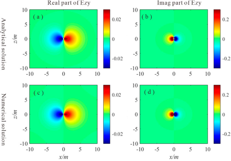
Figure 1. Electromagnetic field distribution of Ezy. (A, B) are the real parts and imaginary of Ezy calculated using the analytical method; (C, D) are the real parts and imaginary of Ezy calculated using the numerical method.

2.4 Spectral domain field characteristics study

In solving for the spatial domain electromagnetic field, the calculation of the spectral domain electromagnetic field is crucial. To investigate this matter, we examined the response characteristics of multi-component signals in the spectral domain under conditions of a uniform medium. In this study, the medium resistivity is set to 10 Ω·m, the signal frequency is 400 kHz, and the spacing is 2 m. The spectral domain responses of the magnetic field signals generated by magnetic dipoles oriented in the x, y, and z directions under these conditions are illustrated in Figure 2. As depicted in this figure, it is evident that the real and imaginary parts of the signals Hxx, Hxz, Hyy, Hxz, and Hzz are even functions in the spectral domain, while Hxy, Hyx, Hyz, and Hzy are odd functions in the spectral domain. Based on this characteristic, the following approximation can be made: The equations should be inserted in editable format from the equation editor.

$H_{*}\left(x,y=y_0,z\right)=\frac{1}{\pi }{\int }_{k_y=0}^{\infty }{\widehat{H}}_{*}{e}^{-i{k}_y{y}_0}d{k}_y$

where ∗ represent xx, xz, yy, zx, zz and $\widehat{H}$ represent the signal in the spectral domain.

$H_{*}\left(x,y=y_0,z\right)=0$

where ∗ represent xy, yx, yz, zy.

Figure 2

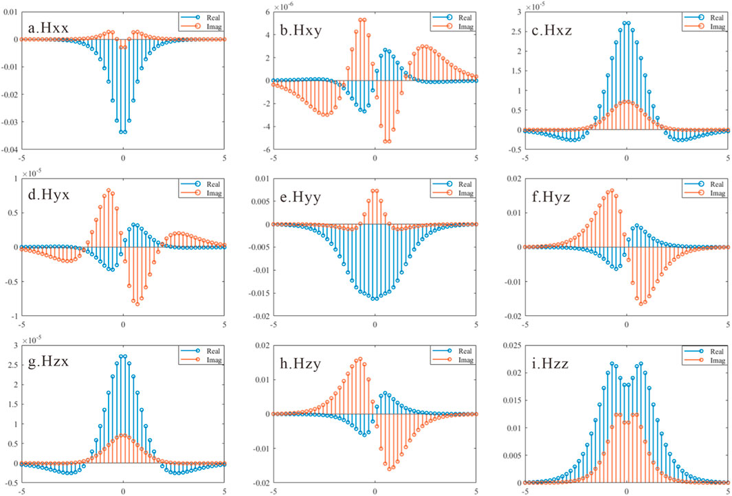
Figure 2. Magnetic dipole response of different components in the spectral domain. (A-C) are the Hxx, Hxy and Hxz signals; (D-F) are the Hyx, Hyy and Hyz signals; (G-I) are the Hzx, Hzy and Hzz signals. The blue lines and red lines represent the real part and the imaginary part of response.

3 Algorithm validation

3.1 1D layered model

As a first example, we establish a three-layer model in Figure 3 to validate the computational accuracy of 2.5D-FEM method. The formation resistivities from top to bottom are 1 Ω·m, 10 Ω·m, 1 Ω·m. The upper and the lower layers are semi-infinite, and the middle layer is 5 m thick. The instrument has drilled from bottom to top with a relative dip angle of 60°. Simulate the induced magnetic field signals with 400 KHz frequency and 2 m spacing.

Figure 3

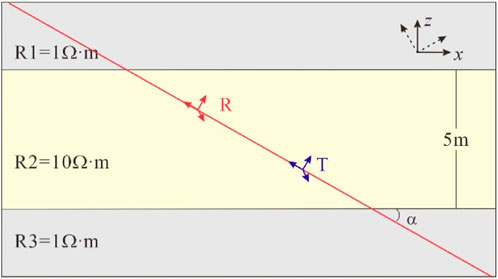
Figure 3. The model of the 1D formation. The red line represent the wellbore trajectory.

The simulated results and relative error are shown in Figures 4, 5, validated with the results computed using an analytical solution. It can be observed that the results of analytical solution and 2.5 FEM are almost equivalent, which indicates the 2.5D FEM is accurate. In addition, the relative errors of the real and imaginary parts of coplanar and coaxial signals are generally less than 1%. A slight increase in error occurs when the instrument passes through the interface, which is attributed to the difference between the equivalent resistivity at the boundary and the actual resistivity. For the orthogonal signals, the mean relative error is close to 1%, with larger errors occurring only when the signal amplitude approaches zero. However, in practical calculations, this does not impact the amplitude ratio or phase difference signals.

Figure 4

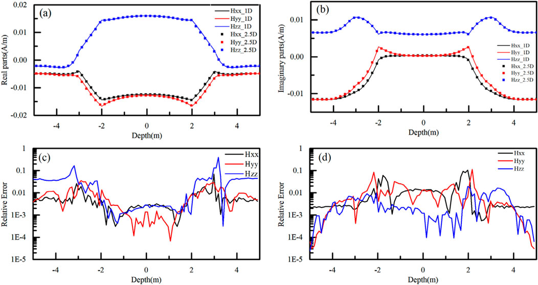
Figure 4. Validation of coplanar an coaxial signals in a 1D layered model. (A, B) are the real parts and imaginary parts of signal, the curves and the scatters are from the analytical solutions and the 2.5D algorithm. (C, D) are the relative errors of real and imaginary parts between the analytical solutions and the 2.5D algorithm.

Figure 5

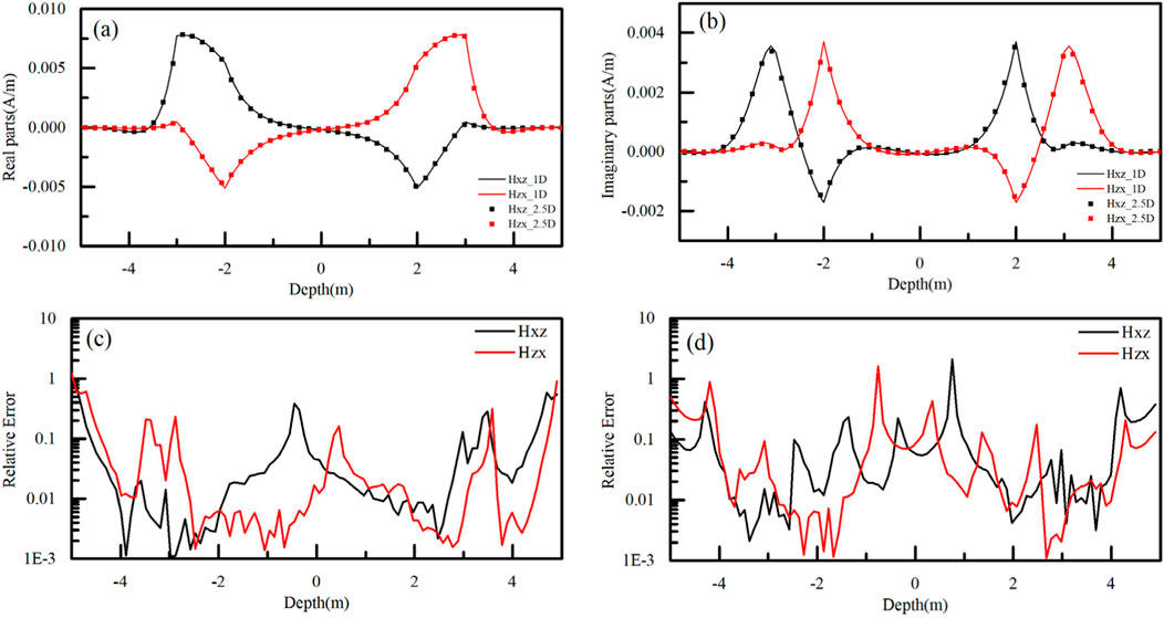
Figure 5. Validation of orthogonal signals in a 1D layered model. (A, B) are the real parts and imaginary parts of signal, the curves and the scatters are from the analytical solutions and the 2.5D algorithm. (C, D) are the relative errors of real and imaginary parts between the analytical solutions and the 2.5D algorithm.

3.2 2D model

To further demonstrate the computational efficiency of the 2.5D FEM, we established a 2D model in Figure 6. The resistivity of formation from top to bottom are 1 Ω·m, 10 Ω·m, 3 Ω·m. Keep the instrument parameters consistent with the previous section, and the corresponding simulation results are shown in Figure 7. This figure compares the results obtained using the 2.5D finite element method with those from the commercial software COMSOL. It can be seen that both methods show good consistency, demonstrating that the 2.5D finite element algorithm can be used to solve the electromagnetic field distribution of 2D models.

Figure 6

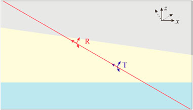
Figure 6. The model of the 2D formation. The red line represents the wellbore trajectory. T and R are the transmitter and receiver.

Figure 7

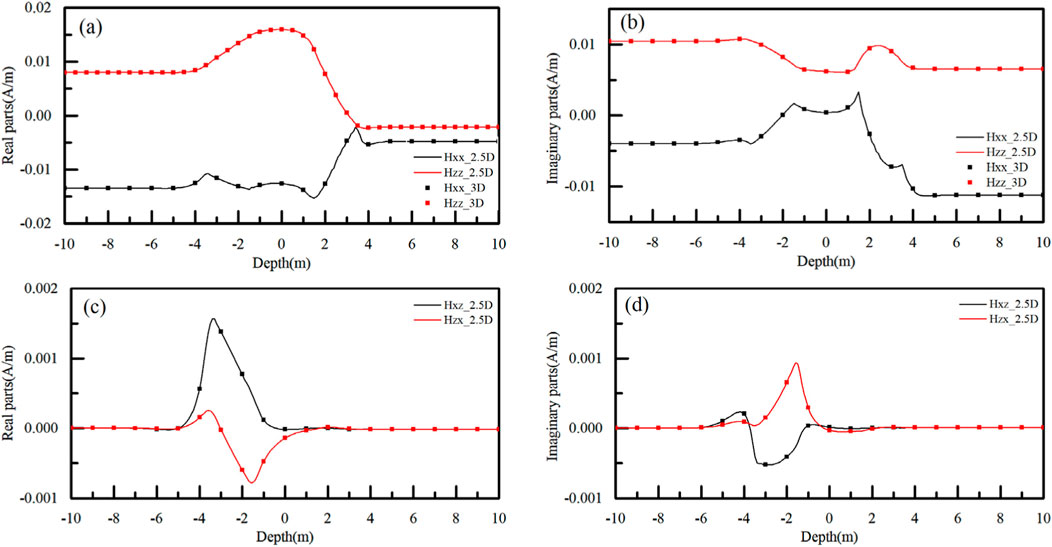
Figure 7. Validation of 2.5D FEM in a 2D model. (A, B) are the real parts and imaginary parts of Hxx and Hzz signals, the curves and the scatters are from the analytical solutions and the 2.5D algorithm. (C, D) are the real parts and imaginary parts of Hxz and Hzx signals. the curves and the scatters are from the analytical solutions and the 2.5D algorithm.

The computation based on the current mesh discretization took a total of 20.23 s. The number of unknowns to be solved is 22,320, with the corresponding matrix size being 22,320 × 22,320, and the number of non-zero elements is 261,764. Additionally, the 2.5D finite element algorithm is based on solving a series of spectral domain 2D problems, with each 2D solution process being independent and non-interfering. This perfectly aligns with the need for parallel computing. Therefore, parallel computation methods can be employed to solve these problems. On a laptop [Intel(R) Core (TM) I7-1360P with 2.20 GHz speed; RAM is 32 GB]. When the number of computation kernel involved in parallel computation is increased from 1 to 12, the computation time per logging point is significantly reduced from 20.23 s to 5.81 s, with the corresponding results shown in Table 1. In contrast, COMSOL requires 362 s, highlighting the significant difference in computational efficiency and fully demonstrating the effectiveness of this method. Moreover, compared to similar 2.5D algorithms (Li et al., 2022), this method has significantly improved computational efficiency. From the table, we can observe that as the number of computation kernel increases, the computational efficiency of this method improves significantly. However, when the number of computation kernel exceeds 6, the acceleration effect on the algorithm becomes less noticeable.

Table 1

Table 1. The parallel computing efficiency under different computation kernel.

4 Analysis of responses in complex model

EDARM is defined through the combination of multi-component signals. In addition to its capability to obtain formation resistivity and anisotropy, it can also detect the interface around and ahead of the instrument, greatly enhancing its geosteering ability. The definition of EDARM for boundary detection as follow:

$\begin{array}{c}USDA=20{\log }_{10}\left|\frac{V_{zz}-V_{zx}}{V_{zz}+V_{zx}}\cdot \frac{V_{zz}+V_{xz}}{V_{zz}-V_{xz}}\right|\\ USDP=-angle\left(\frac{V_{zz}-V_{zx}}{V_{zz}+V_{zx}}\cdot \frac{V_{zz}+V_{xz}}{V_{zz}-V_{xz}}\right)\end{array}$

$\begin{array}{cc}UHRA=20{\log }_{10}\left|\frac{2V_{zz}}{V_{xx}+V_{yy}}\right|& UHRP=-angle\left(\frac{2V_{zz}}{V_{xx}+V_{yy}}\right)\end{array}$

where the USDA and USDP represent the attenuation (ATT) and phase shift (PS) of Look-around mode, the UHRA and UHRP represent the ATT and PS of Look-ahead mode.

To facilitate the explanation of the detection characteristics of Geosphere under different formation model, we adopt the fault and wedge models, which are commonly encountered in actual drilling scenarios (as shown in Figure 8).

Figure 8

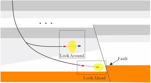
Figure 8. The formation model of EDARM. The black line represents the wellbore trajectory. The Look-around and Look-ahead measurement scenarios have been shown in this Figure.

4.1 Fault model

Faults play a crucial role in the migration and accumulation of oil and gas, presenting a significant challenge in geosteering. Accurately identifying the location of the interface ahead of the instrument is essential to prevent the drill bit from penetrating the reservoir. To investigate the impact of fault structures on logging responses, a model, as shown in Figure 9, has been developed. Three structural parameters are defined to characterize fault variations: the relative vertical displacement (H) between the upper and lower fault blocks, the distance (D) from the instrument to the fault boundary, and the angle (θ) between the fault plane and the formation interface. Assuming an instrument spacing of 8 m, a signal frequency of 24 kHz, and formation resistivities of 4 Ω·m, 20 Ω·m, and 2 Ω·m (from top to bottom), with a 10 m thick middle layer, the instrument is drilled horizontally from left to right.

Figure 9

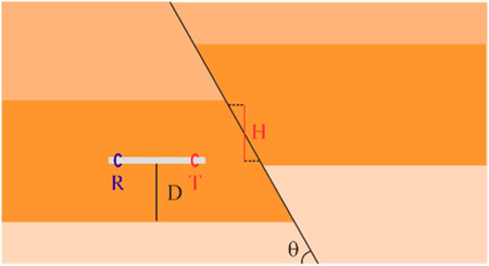
Figure 9. The fault model and parameters.

4.1.1 Relative vertical displacement

Assuming the distance (D) from the instrument to the boundary is set at 5 m, and the angle between the fault plane and the formation interface is fixed at 30°, the responses of the Look-ahead and Look-around modes were simulated for various relative vertical displacements (H) ranging from 6 m to 9 m. The simulation results are shown in Figure 10, where the x-axis represents the horizontal position of the transmitter, with the fault plane located at x = 0 m. As illustrated in the figure, when the instrument approaches the fault plane at a fixed distance from the upper and lower interfaces (x < 0 m), the Look-around mode signals remain constant, exhibiting no significant abnormalities. However, once the instrument drills through the fault plane (x > 0 m), a noticeable anomaly appears, with the signal difference becoming more pronounced as the instrument nears the interface. In contrast, the Look-ahead mode signals show a clear declining trend as the instrument approaches the fault plane. The signal difference becomes more pronounced as the H value increases. Specifically, at H = 9 m, the UHRA and UHRP signals are able to identify the fault plane at distances of 4.6 m and 3.45 m ahead, respectively. Overall, circumferential measurement signals are primarily influenced by the borehole wall interface and are unable to effectively represent the interface ahead of the instrument. In contrast, the signals of Look-around can accurately identify the interface ahead of the drill bit.

Figure 10

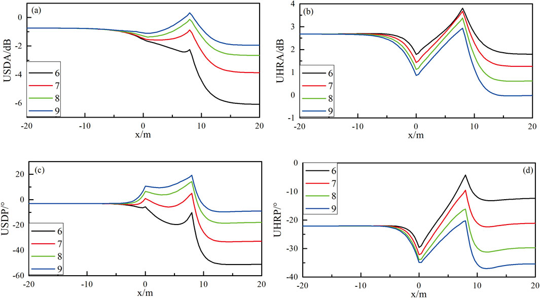
Figure 10. The responses of fault model under different H. (A, C) represent the ATT and PS signals of Look-around mode; (B, D) represent the ATT and PS signals of Look-ahead mode.

4.1.2 Inclination angle

The previous analysis revealed that the Look-around and Look-ahead modes exhibit distinct response patterns to the fault plane. To further investigate the relationship between the measurement signals and the instrument’s position relative to the interface, additional simulations were conducted. In these simulations, the instrument parameters were held constant, with the DTB fixed at 1 m and H at 5 m. The distance from the instrument to the fault plane (x) was varied from 2 m to 5 m, while the inclination angle (θ) was considered within a range of 45°–135°. The instrument’s position was fixed, and the responses were simulated across varying inclination angles (θ). The results are presented in Figure 11.

Figure 11

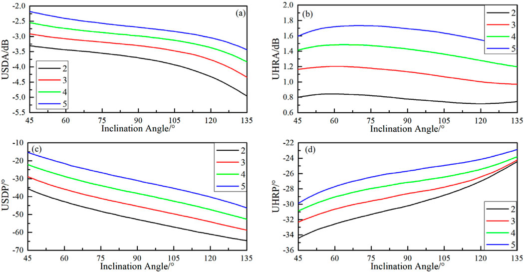
Figure 11. The responses of fault model under different angle. (A, C) represents the ATT and PS signals of Look-around mode; (B, D) represents the ATT and PS signals of Look-ahead mode.

The simulations show that both the Look-ahead and Look-around signals exhibit regular variations with changes in the fault plane’s inclination angle. Specifically, the Look-around signal decreases as the inclination angle increases, demonstrating a negative correlation. In contrast, the Look-ahead signal displays more complex behavior with changes in the inclination angle. Among the Look-ahead signals, the amplitude ratio signal (UHRA) is relatively insensitive to the inclination angle, while the phase difference signal (UHRP) shows a strong positive correlation. Overall, both Look-ahead and Look-around measurement signals exhibit clear and consistent trends with respect to the inclination angle, indicating a discernible relationship that warrants further exploration.

The Look-around and Look-ahead detection mode signals were combined under identical geological model conditions to generate crossplots, as shown in Figure 12. In these plots, the x-axis represents the signals of Look-around detection mode, while the y-axis represents the signal of Look-ahead detection mode. The dashed line indicates the distance from the instrument to the fault plane, and the solid line represents the fault plane’s inclination angle. The crossplots clearly show that the solid and dashed lines intersect, dividing the plot into distinct zones. During the geosteering process, resistivity characteristics often vary due to the inherent properties of the rock. These resistivity values can be derived using inversion algorithms. Based on this, the corresponding intersection chart can be selected, and the position of the measured data points on the chart can be used to approximate both the distance and the angle between the instrument and the fault plane. Furthermore, a comparison of the two crossplots reveals that, when the fault plane’s dip angle is small, the amplitude ratio crossplot is confined to a smaller region, indicating lower signal sensitivity. In contrast, the phase difference signal distribution is more evenly spread across regions, making it easier to detect changes in both the fault dip angle and the distance from the instrument to the fault plane.

Figure 12

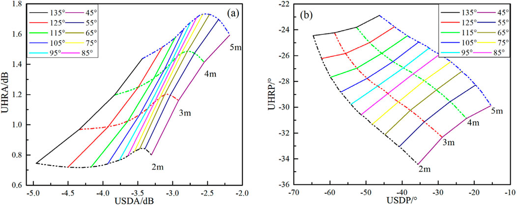
Figure 12. The crossplots of Look-around and Look-ahead signals in fault model. (A, B) are the crossplots of ATT and PS signals. The solid lines represent the inclination angle, the dashed lines represent the distance between the instrument and boundary.

4.2 Wedge model

The angles of the upper and lower formation interfaces differ are commonly occur in geosteering study. The wedge model, as shown in Figure 13, is used to investigate the impact of interface dip angle changes on measurement signals. In this model, the instrument is assumed to be parallel to the upper interface and forms an angle α with the lower interface. With the instrument fixed at a distance of 8 m from the upper interface, and maintaining constant instrument parameters and formation resistivity, simulations were conducted for both Look-around and Look-ahead responses under varying α values, as shown in Figure 14.

Figure 13

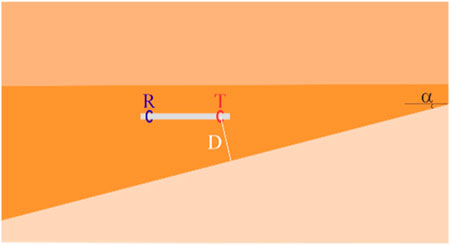
Figure 13. The wedge model and parameters.

Figure 14

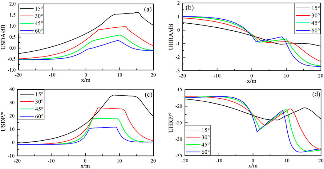
Figure 14. The responses of wedge model under different angle. (A, C) represents the ATT and PS signals of Look-around mode; (B, D) represents the ATT and PS signals of Look-ahead mode.

The figures clearly demonstrate that as the angle α increases, the strength of the Look-around detection signal gradually decreases, while the strength of the Look-ahead detection signal increases. Similar to the earlier analysis of fault structures, a noticeable separation between the curves is observed at different angles. This behavior suggests that a crossplot can be used to assess the relative position of the instrument in relation to the formation interface.

Figure 15 presents a crossplot of the Look-around and Look-ahead signals. The axes of this plot are consistent with those in Figure 15, where the solid line represents the angle between the instrument and the formation interface, and the dashed line indicates the perpendicular distance from the transmitting antenna to the interface. The plot clearly shows that the curves intersect, dividing the plot into several regions. Notably, when the angle is larger and the distance to the interface is shorter, the occupied area expands, making it easier to extract the corresponding values from the crossplot.

Figure 15

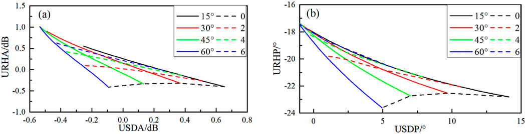
Figure 15. The crossplots of Look-around and Look-ahead signals in wedge model. (A, B) are the crossplots of ATT and PS signals. The solid lines represent the inclination angle, the dashed lines represent the distance between the instrument and boundary.

5 Discussion

This study introduces a novel 2.5D FEM fast forward algorithm, along with simulations tailored for specific drilling geological orientation scenarios, which offer new insights into signal processing and interface identification. The new algorithm significantly improves computational efficiency by using a pseudo-Dirac function for the signal source equivalence and signal spectrum domain analysis. With the integration of parallel computing, the computation time for a single point is reduced to under 6 s, offering improved efficiency compared to other algorithms. In addition, for specific fault model and wedge model analysis, a fast identification method for interface position and angle is proposed for the first time. This method is applicable to most scenarios in drilling geological orientation. The fast and efficient forward algorithm, along with the simple interface identification method, provides algorithmic support and initial value optimization for the inversion of formation interfaces. This approach effectively addresses the issue of low processing efficiency in existing ultra-deep geological orientation.

Data availability statement

The original contributions presented in the study are included in the article/Supplementary Material, further inquiries can be directed to the corresponding author.

Author contributions

PZ: Conceptualization, Data curation, Formal Analysis, Funding acquisition, Investigation, Methodology, Resources, Supervision, Validation, Visualization, Writing–original draft, Writing–review and editing. SD: Funding acquisition, Methodology, Resources, Validation, Writing–original draft. XY: Formal Analysis, Methodology, Visualization, Writing–review and editing. FL: Data curation, Funding acquisition, Validation, Writing–review and editing. WX: Data curation, Supervision, Validation, Visualization, Writing–review and editing.

Funding

The author(s) declare that financial support was received for the research, authorship, and/or publication of this article. This research was funded by Natural Science Foundation of Xinjiang Uygur Autonomous Region (2022D01B140 and 2021D01E22), Research Foundation of China University of Petroleum-Beijing at Karamay (XQZX20230009), National Natural Science Foundation of China (42204121), Research project of the Tianchi Talent Introduction Plan in Xinjiang Uygur Autonomous Region and Karamay Science and Technology Plan Project (Innovative Talents) 20232023hjcxrc0052.

Conflict of interest

Author XY was employed by Sinopec Matrix Corporation.

The remaining authors declare that the research was conducted in the absence of any commercial or financial relationships that could be construed as a potential conflict of interest.

Generative AI statement

The author(s) declare that no Generative AI was used in the creation of this manuscript.

Publisher’s note

All claims expressed in this article are solely those of the authors and do not necessarily represent those of their affiliated organizations, or those of the publisher, the editors and the reviewers. Any product that may be evaluated in this article, or claim that may be made by its manufacturer, is not guaranteed or endorsed by the publisher.

Supplementary material

The Supplementary Material for this article can be found online at: https://www.frontiersin.org/articles/10.3389/feart.2025.1506238/full#supplementary-material

References

Bakr, S. A., Pardo, D., and Torres-Verdín, C. (2017). Fast inversion of logging-while-drilling resistivity measurements acquired in multiple wells. Geophysics 82 (3), E111–E120. doi:10.1190/geo2016-0292.1

CrossRef Full Text | Google Scholar

Bell, C., Hampson, J., Eadsforth, P., Chemali, R., Helgesen, T., Meyer, H., et al. (2006). “Navigating and imaging in complex geology with azimuthal propagation resistivity while drilling,” in SPE annual technical conference and exhibition, SPE–102637.

Google Scholar

Bittar, M., and Aki, A. (2015). Advancement and economic benefit of geosteering and well-placement technology. Lead. Edge 34 (4), 524–528. doi:10.1190/tle34050524.1

CrossRef Full Text | Google Scholar

Bittar, M., Klein, J., Beste, R., Hu, G., Wu, M., Pitcher, J., et al. (2009). A new azimuthal deep-reading resistivity tool for geosteering and advanced formation evaluation. SPE Reserv. Eval. & Eng. 12 (02), 270–279. doi:10.2118/109971-pa

CrossRef Full Text | Google Scholar

Constable, M. V., Antonsen, F., Stalheim, S. O., Olsen, P. A., Fjell, Ø. Z., Dray, N., et al. (2016). “Looking ahead of the bit while drilling: from vision to reality,” in SPWLA 57th annual logging symposium.

Google Scholar

Davydycheva, S., Druskin, V., and Habashy, T. (2003). An efficient finite-difference scheme for electromagnetic logging in 3D anisotropic inhomogeneous media. Geophysics 68 (5), 1525–1536. doi:10.1190/1.1620626

CrossRef Full Text | Google Scholar

Davydycheva, S., Torres-Verdín, C., Hou, J., Saputra, W., Rabinovich, M., Antonsen, F., et al. (2023). “3D electromagnetic modeling and quality control of ultradeep borehole azimuthal resistivity measurements,” in SPWLA annual logging symposium (Lake Conroe, Texas, USA: SPWLA), D041S013R002.

Google Scholar

Dupuis, C., and Denichou, J. M. (2015). Automatic inversion of deep-directional-resistivity measurements for well placement and reservoir description. Lead. Edge 34 (5), 504–512. doi:10.1190/tle34050504.1

CrossRef Full Text | Google Scholar

Hagiwara, T. (2018). “Detection sensitivity and new concept of deep reading look-ahead look-around geosteering tool,” in SEG international exposition and annual meeting (Anaheim, California, USA: October).

Google Scholar

Hartmann, A., Vianna, A., Maurer, H. M., Sviridov, M., Martakov, S., Lautenschläger, U., et al. (2014). “Verification testing of a new extra-deep azimuthal resistivity measurement,” in SPWLA annual logging symposium.

Google Scholar

Hu, X., and Fan, Y. (2018). Huber inversion for logging-while-drilling resistivity measurements in high angle and horizontal wells. Geophysics 83 (4), D113–D125. doi:10.1190/geo2017-0459.1

CrossRef Full Text | Google Scholar

Hu, X. F., Fan, Y. R., Wu, F., Lei, W., and XiYong, Y. (2018). Fast multiple parameter inversion of azimuthal LWD electromagnetic measurement. Chin. J. Geophys. 61 (11), 4690–4701. doi:10.6038/cjg2018L0746

CrossRef Full Text | Google Scholar

Iverson, M., Fejerskov, M., Skjerdingstad, A., Clark, A. J., Denichou, J. M., Ortenzi, L., et al. (2004). Geosteering using ultradeep resistivity on the Grane field, Norwegian North Sea. Petrophysics 45 (3), 232–240.

Google Scholar

Jahani, N., Torres-Verdín, C., and Hou, J. (2023). Limits of three-dimensional target detectability of logging while drilling deep-sensing electromagnetic measurements from numerical modelling. Geophys. Prospect. 72, 1146–1162. doi:10.1111/1365-2478.13451

CrossRef Full Text | Google Scholar

Larsen, D. S., Hartmann, A., Luxey, P., Martakov, S., Skillings, J., Tosi, G., et al. (2015). “Extra-deep azimuthal resistivity for enhanced reservoir navigation in a complex reservoir in the Barents Sea,” in SPE annual technical conference and exhibition. September.

Google Scholar

Li, H., Wu, Z., and Yue, X. (2022). A near-optimal quadrature for 2.5 D EM logging-while-drilling tool modeling. J. Appl. Geophys. 207, 104841. doi:10.1016/j.jappgeo.2022.104841

CrossRef Full Text | Google Scholar

Li, H., and Zhou, J. (2017). “Distance of detection for LWD deep and ultra-deep azimuthal resistivity tools,” in SPWLA annual logging symposium (Oklahoma City, Oklahoma, USA: SPWLA. June), D053S013R009.

Google Scholar

Li, Q., Omeragic, D., and Chou, L. E. F. (2005). “New directional electromagnetic tool for proactive geosteering and accurate formation evaluation while drilling,” in SPWLA annual logging symposium (SPWLA). SPWLA-2005-UU.

Google Scholar

Li, S., Chen, J., and Binford, J. R. (2014). “Using new LWD measurements to evaluate formation resistivity anisotropy at any dip angle,” in SPWLA annual logging symposium (Abu Dhabi, United Arab Emirates: SPWLA). SPWLA-2014-EEEE.

Google Scholar

Liang, P., Di, Q., Chen, W., Zhang, W., Liu, R., and Li, X. (2023). An EM LWD tool for deep reading looking-ahead. IEEE Access 11, 142601–142610. doi:10.1109/access.2023.3339777

CrossRef Full Text | Google Scholar

Lu, H., Shen, Q., Chen, J., Wu, X., and Fu, X. (2019). Parallel multiple-chain DRAM MCMC for large-scale geosteering inversion and uncertainty quantification. J. Petroleum Sci. Eng. 174, 189–200. doi:10.1016/j.petrol.2018.11.011

CrossRef Full Text | Google Scholar

Noh, K., Pardo, D., and Torres-Verdín, C. (2021). 2.5-D deep learning inversion of LWD and deep-sensing EM measurements across formations with dipping faults[J]. IEEE Geoscience Remote Sens. Lett. 19, 1–5. doi:10.1109/lgrs.2021.3128965

CrossRef Full Text | Google Scholar

Omeragic, D., Li, Q., Chou, L., Yang, L., Duong, K., Smits, J. W., et al. (2005). Deep directional electromagnetic measurements for optimal well placement. Dallas, Texas, USA: SPE Annual Technical Conference and Exhibition.

CrossRef Full Text | Google Scholar

Pardo, D., and Torres-Verdín, C. (2015). Fast 1D inversion of logging-while-drilling resistivity measurements for improved estimation of formation resistivity in high-angle and horizontal wells. Geophysics 80 (2), E111–E124. doi:10.1190/geo2014-0211.1

CrossRef Full Text | Google Scholar

Rodríguez-Rozas, Á., and Pardo, D. (2016). A priori Fourier analysis for 2.5 D finite elements simulations of logging-while-drilling (LWD) resistivity measurements. Procedia Comput. Sci. 80, 782–791. doi:10.1016/j.procs.2016.05.368

CrossRef Full Text | Google Scholar

Rodríguez-Rozas, Á., Pardo, D., and Torres-Verdín, C. (2018). Fast 2.5 D finite element simulations of borehole resistivity measurements. Comput. Geosci. 22, 1271–1281. doi:10.1007/s10596-018-9751-7

CrossRef Full Text | Google Scholar

Seydoux, J., Legendre, E., Mirto, E., Dupuis, C., Jean-Michel, D., Bennett, N., et al. (2014). Full 3D deep directional resistivity measurements optimize well placement and provide reservoir-scale imaging while drilling. In SPWLA annual logging symposium Abu Dhabi, United Arab Emirates: SPWLA-2014.

Google Scholar

Thiel, M., Bower, M., and Omeragic, D. (2018). 2D reservoir imaging using deep directional resistivity measurements. Petrophysics 59 (02), 218–233. doi:10.30632/pjv59n2-2018a7

CrossRef Full Text | Google Scholar

Wang, L., Deng, S., Zhang, P., Cao, Y. C., Fan, Y. R., and Yuan, X. Y. (2019a). Detection performance and inversion processing of logging-while-drilling extra-deep azimuthal resistivity measurements. Petroleum Sci. 16 (5), 1015–1027. doi:10.1007/s12182-019-00374-4

CrossRef Full Text | Google Scholar

Wang, L., and Fan, Y. (2019). Fast inversion of logging-while-drilling azimuthal resistivity measurements for geosteering and formation evaluation. J. Petroleum Sci. Eng. 176, 342–351. doi:10.1016/j.petrol.2019.01.067

CrossRef Full Text | Google Scholar

Wang, L., Fan, Y. R., Huang, R., Yu-Jiao, H., Zhen-Guan, W., Dong-Hui, X., et al. (2015). Three dimensional Born geometrical factor of multi-component induction logging in anisotropic media. Acta Phys. Sin. 64 (23), 239301. doi:10.7498/aps.64.239301

CrossRef Full Text | Google Scholar

Wang, L., Li, H., and Fan, Y. R. (2019b). Bayesian inversion of logging-while-drilling extra-deep directional resistivity measurements using parallel tempering Markov chain Monte Carlo sampling. IEEE Trans. Geoscience Remote Sens. 57 (10), 8026–8036. doi:10.1109/tgrs.2019.2917839

CrossRef Full Text | Google Scholar

Wu, H. H., Golla, C., Parker, T., Clegg, N., and Monteilhet, L. (2018). “A new ultra-deep azimuthal electromagnetic LWD sensor for reservoir insight,” in SPWLA annual logging symposium (London, UK: SPWLA).

Google Scholar

Wu, Z., Fan, Y., Wang, J., Zhang, R., and Liu, Q. H. (2019). Application of 2.5-D finite difference method in logging-while-drilling electromagnetic measurements for complex scenarios. IEEE Geoscience Remote Sens. Lett. 17(4): 577–581. doi:10.1109/lgrs.2019.2926740

CrossRef Full Text | Google Scholar

Wu, Z., Li, H., Han, Y., Zhang, R., Zhao, J., and Lai, Q. (2022). Effects of formation structure on directional electromagnetic logging while drilling measurements. J. Petroleum Sci. Eng. 211, 110118. doi:10.1016/j.petrol.2022.110118

CrossRef Full Text | Google Scholar

Wu, Z. G., Li, H., and Yue, X. Z. (2023). 2.5-Dimensional modeling of EM logging-while-drilling tool in anisotropic medium on a Lebedev grid. Petroleum Sci. 20(1): 249–260. doi:10.1016/j.petsci.2022.09.010

CrossRef Full Text | Google Scholar

Wu, Z. G., Wang, L., Fan, Y. R., Deng, S. G., Huang, R., and Xing, T. (2020). Detection performance of azimuthal electromagnetic logging while drilling tool in anisotropic media. Appl. Geophys. 17 (1), 1–12. doi:10.1007/s11770-020-0804-z

CrossRef Full Text | Google Scholar

Xia, X., Persello, C., and Koeva, M. (2019). Deep fully convolutional networks for cadastral boundary detection from UAV images. Remote Sens. 11 (14), 1725. doi:10.3390/rs11141725

CrossRef Full Text | Google Scholar

Zhang, P., Deng, S., Hu, X., et al. (2021). Detection performance and inversion processing of logging-while-drilling extra-deep azimuthal resistivity measurements. Chin. J. Geophys. 64 (6), 2210–2219.

Google Scholar

Zhao, N., Li, N., Xiao, Z., Wang, X., and Qin, C. (2024). Physics-driven deep learning pixel-based inversion of logging-while-drilling in anisotropic formation. IEEE Trans. Geoscience Remote Sens. 62, 1–12. doi:10.1109/tgrs.2024.3355463

CrossRef Full Text | Google Scholar