Logging-data-driven lithology identification in complex reservoirs: an example from the Niuxintuo block of the Liaohe oilfield

For lithologic oil reservoirs, lithology identification plays a significant guiding role in exploration targeting, reservoir evaluation, well network adjustment and optimization, and the establishment of reservoir models. Lithology is usually predicted from well log data based on limited core observations. In recent years, machine learning algorithms have been applied to lithology identification to enhance prediction accuracy. In this paper, five algorithms, including Bayes discriminant analysis, Random Forest (RF), Support Vector Machine (SVM), Back Propagation Neural Network (BPNN), and Convolutional Neural Network (CNN) are evaluated for lithology identification using data from the Niuxintuo reservoir. This reservoir is characterized by complex structural and sedimentary features, strong heterogeneity, and intricate lithological properties, all of which present considerable challenges for well logging identification. First, we conducted a detailed observation of the core lithology. Based on the requirements for reservoir evaluation and the principles of logging identification, we reclassify the lithology of the study area into two categories: clastic rocks and dolomite. The clastic rocks are further subdivided into five rock types: fine sandstone, medium-coarse sandstone, conglomerate, mudstone, and transitional rock. The well log series were selected through sensitivity analysis. Then, Bayes discriminant analysis and four machine learning methods were trained to identify the lithology of the study area. The results indicate that except for Bayes discriminant analysis, all the constructed machine learning classifiers demonstrate high prediction accuracy, with the accuracy rate exceeding 85%. Among them, SVM classifier shows the best performance achieving a prediction accuracy as high as 93%. Additionally, the well-trained SVM model was successfully used to predict the lithology profile of blind wells. Our findings provide valuable guidance for predicting the remaining oil distribution and further exploration potential in the Niuxintuo oilfield. Furthermore, this study gains insight into the process and methodology of rapidly predicting lithology of hydrocarbon reservoirs using easily accessible well logging data.

1 Introduction

Lithology identification is a crucial issue in reservoir characterization, as it helps correlate critical reservoir properties such as porosity, permeability and oil saturation, and plays a vital role in constructing field-scale reservoir models. Well log data have advantages such as high vertical resolution, good continuity, and convenient data acquisition. Therefore, they are an important resource for obtaining underground lithological information. Lithology classification based on well log data forms the foundation for reservoir characterization and provides a basis for geological studies such as sedimentary facies and environmental analysis. In addition to its significance in formation evaluation and geological analysis, lithology interpretation plays an important role in predicting sweet spot reservoirs and forecasting remaining oil distribution. The traditional methods for interpreting lithology mainly include cross-plot technique (e.g., Sanyal et al., 1980), curve feature method (Anifowose et al., 2019), imaging logging chart method (Cohn et al., 1996), multiple linear regression method (Delfiner et al., 1987), and discriminant analysis method (Dong et al., 2016; Dong et al., 2022). However, each of the method have some limitations (Sun et al., 2019). For example, a lack of clarity in the relationships between the data points may result in the cross-plot technique failed. Moreover, and it cannot display higher dimensional spatial information, and usually only two parameters can be considered at the same time (McDowell et al., 1998). Multiple linear regression method is very sensitive to highly correlated independent variables, and the relationship between variables is often nonlinear, which may lead to a decrease in the explanatory power of the model (Delfiner et al., 1987). Discriminant analysis methods require a large number of high-quality datasets, and are limited by some assumed premises (Dong et al., 2016). Overall, these methods generally require a large number of samples, which are very time-consuming. Recognizing lithology boundaries from well log data is inherently a nonlinear problem, primarily because log curves are influenced by rock properties like pore fluids. Therefore, it is essential to develop a suitable nonlinear approach that can effectively address these challenges.

The rapid advancement of computer technology has enabled machine learning methods to offer more time and cost-effective solutions with higher lithology identification accuracy, compared to traditional lithology identification methods (e.g., Ashraf et al., 2021; Bressan et al., 2020). Nowadays, numerous machine learning methods have emerged and been successfully applied to lithology identification (e.g., Wang et al., 2014; Bhattacharya et al., 2016; Biau and Scornet, 2016; Saporetti et al., 2018; Wang et al., 2020; Zhang et al., 2023). Machine learning can be categorized into three types: unsupervised learning, semi-supervised learning, and supervised learning. Unsupervised learning techniques, such as expectation maximisation (Miyahara et al., 2020), K-mean clustering (Huang et al., 2016), hierarchical clustering (Vichi et al., 2022), and deep autocoders (Kampffmeyer et al., 2018), are used only by arranging the lithology according to its intrinsic characteristics to provide an overall perspective. They are helpful when the dataset is limited (there are no available labels). In contrast, semi-supervised learning techniques (SSL), such as forward and unlabeled machine learning (Helm et al., 2023), active semi-supervised algorithms (Xu et al., 2021a; Shan et al., 2021), and Laplace Support Vector Machines (Yang and Xu, 2018), are beneficial when there is a limited amount of labelled data accessible. On the contrary, supervised learning techniques, which are suitable for learning a pattern in a known labelled species and inferring new instances in accordance with this pattern, can provide precise training data and therefore give very accurate results (Jordan and Mitchell, 2015). Several well-known supervised shallow learning algorithms are used for petrographic classification of core-tagging-based logs. This category includes backpropagation neural networks (Amari, 1993; Dong et al., 2023), support vector machine (SVM) (Wang et al., 2014), K-nearest neighbours (Wang et al., 2023; Li et al., 2024), and decision trees (DT) (Zhou et al., 2020). In addition, uniform integration techniques such as Random Forest (RF) (Yan et al., 2024), Extreme Gradient Boosting (Chen and Guestrin, 2016; Zheng et al., 2022), and Logistic Boosting Regression (Huang et al., 2019) belong to the same category, and such supervised algorithms use geological rules to make petrographic estimation more credible. In addition, several popular deep learning (DL) algorithms (Goodfellow et al., 2016; Miclea et al., 2020), such as convolutional neural networks (Xu et al., 2021b), recurrent neural networks (Tian et al., 2021) and long- and short-term memory networks (Lin et al., 2020), and TabNet (Madani et al., 2018; Li et al., 2022), possess very excellent properties such as weight sharing, local connectivity, and translational isotropy to effectively handle high-dimensional data.

The Niuxintuo reservoir is a typical lithological reservoir. Previous studies have shown that sedimentary environments significantly influence the lithology distribution. Moreover, the lithology controls petrophysical properties, and petrophysical properties control oil saturation (Zhou, 2022; Li, 2022). In this article, we applied multiple methods for lithology identification in the study area and select the most appropriate method for lithology prediction. Firstly, based on the detailed observation and description of rock cores, the lithology of the Niuxintuo area in is divided into six categories: fine sandstone, medium coarse sandstone, conglomerate, mudstone, transitional rock, and dolomite. Subsequently, the logging sequence is standardized and normalized to eliminate systematic errors, thereby improving the accuracy in describing, interpreting, and predicting reservoirs. Building on this, extensive cross plots are employed to evaluate the sensitivity of logging sequences. By integrating lithology sensitivity, data reliability, and curve complementarity, six key parameters—acoustic transmit time (AC), compensated neutron (CNL), density (DEN), gamma ray (GR), resistivity (RT), and conductivity (CON_CAL)—are selected as predictive curves for lithology identification. The initial step in multi-method lithology identification involves classifying lithology using Bayes discriminant analysis. However, with a prediction accuracy of only 58.20%, this approach falls short of meeting the requirements for reliable lithology prediction. Then, the focus shifted to exploring lithology identification using advanced machine learning algorithms, including RF, SVM, BPNN, and CNN. The developed machine learning classifiers demonstrate high prediction accuracy, with SVM achieving the best performance, boasting a prediction accuracy of up to 93%. The findings offer crucial guidance for forecasting remaining oil distribution and evaluating further exploration potential in the Niuxintuo oilfield. Moreover, this study provides valuable insights into the methodology and process of rapidly predicting hydrocarbon reservoir lithology using a large amount of logging data.

2 Methodology

This section provides a detailed overview of lithology identification methods, including core lithology observation and statistics, well logging data preprocessing, Bayes discriminant analysis, and four machine learning methods for lithology identification. The overall workflow is show in Figure 1.

Figure 1

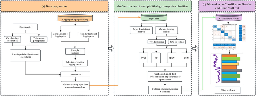
Figure 1. Lithology identification flowchart of this study. (A) Data preparation. (B) Construction of multiple lithology recognition classifiers. (C) Discussion on Classification Resultsand Blind Well test.

2.1 Core lithology observation and statistics

The lithology types of Niuxintuo Oilfield are complex. Based on the detailed observation of core samples along with thin section data, the lithology types in the study area are summarized. Overall, the lithology of Niuxintuo reservoir can be divided into two categories: one is the alluvial fan type clastic rock composed of fine sandstone, siltstone, medium sandstone, coarse sandstone, and gravel rock; The other type is laminated dolomite and muddy dolomite with transitional fan edge lake facies (Figures 2, 3).

Figure 2

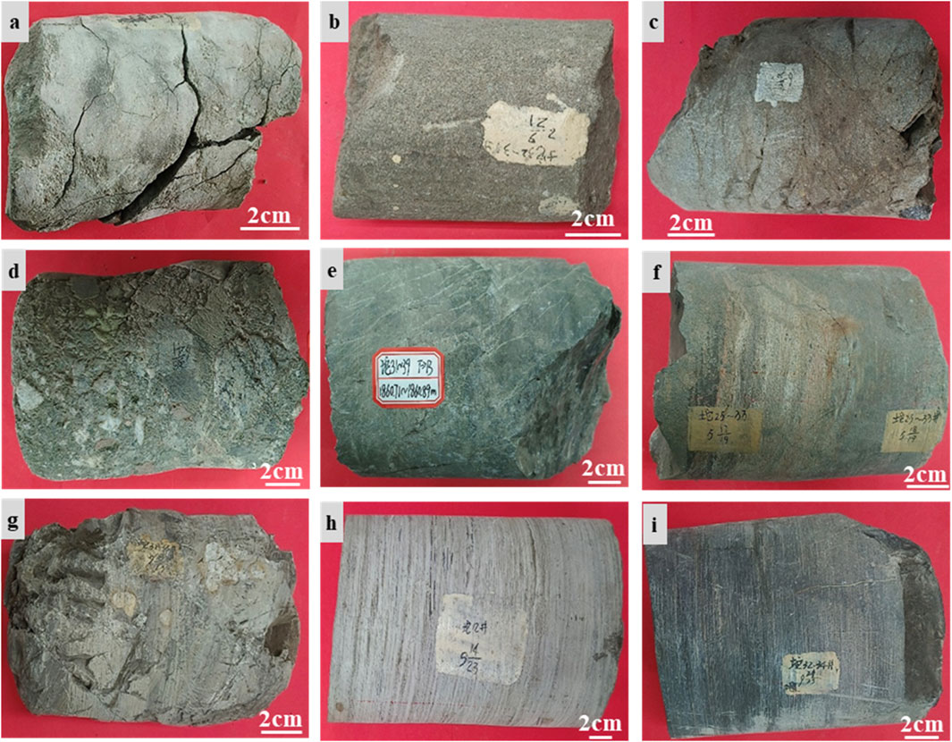
Figure 2. Typical core photographs for different lithologies of Niuxintuo reservoir. (A) Tuo22,1693.72 m, fine sandstone; (B) Tuo 32–34, 1713.56 m, medium sandstone; (C) Tuoguan 2, 1790.08 m, coarse sandstone; (D) Tuo 22, 1707.66 m, gravel rock; (E) Tuo 31–39, 1860.71 m, argillaceous limestone; (F) Tuo 25–33, 2,328.86 m, silty mudstone; (G) Tuo 32–34, 1745.69 m, argillaceous dolomite; (H) Tuo 12, 2,103.66 dolomite; (I) Tuo 32–34, 1748.77 m, dolomitic mudstone.

Figure 3

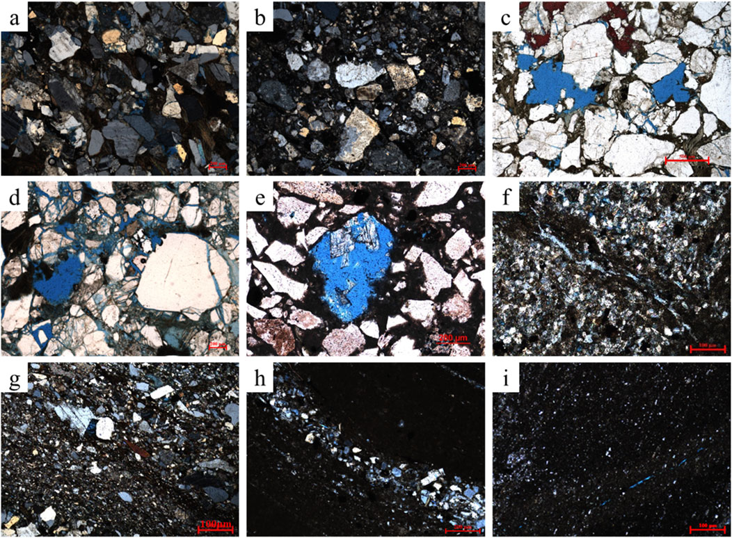
Figure 3. Casting thin section of different lithologies. (A) Tuo 31–39, 1,690.28 m, fine sandstone; (B) Tuo 25–33, 2,396.43 m, gravelly fine sandstone; (C) Tuo 31–39, 1785.74 m, medium sandstone; (D) Tuo 14, 1,557.87 m, coarse sandstone; (E) Tuo 25–33, 2,324.63 m, conglomerate; (F) Tuo 25–33, 2,321.46 m, silty mudstone; (G) Tuo 31–39, 1719.58 m, fine sand mixed with mudstone; (H) Tuo 12, 1,663.19 m, dolomite; (I) Tuo 32–34, 1745.6 m, muddy dolomite.

Furthermore, through the observation of cast thin sections and analysis of mineral composition, genetic processes, compositional content, and sedimentary structures, the lithology has been further subdivided into 19 fundamental rock types (Table 1).

Table 1

Table 1. Lithology types of the niuxintuo oil reservoir.

Cross plot is the most commonly used method for displaying the relationships between variables and is widely used in reservoir research (Ehsan and Gu, 2020). It can display different logging data on the same plane and evaluate the relationships between these data through the position and shape of the intersection points. Accurate lithology identification and characterization require first understanding the physical property differences among various rock types, followed by selecting suitable logging parameters for quantitative differentiation.

Using the preprocessed logging sequences and core lithology labels, a cross-plot analysis was conducted to identify lithology-sensitive logging curves (Figure 4). Considering lithology sensitivity, data quality reliability, and curve complementarity, AC, CNL, DEN, GR, RT, and CON_CAL were selected as lithology-sensitive curves for subsequent research on logging-based lithology identification.

Figure 4

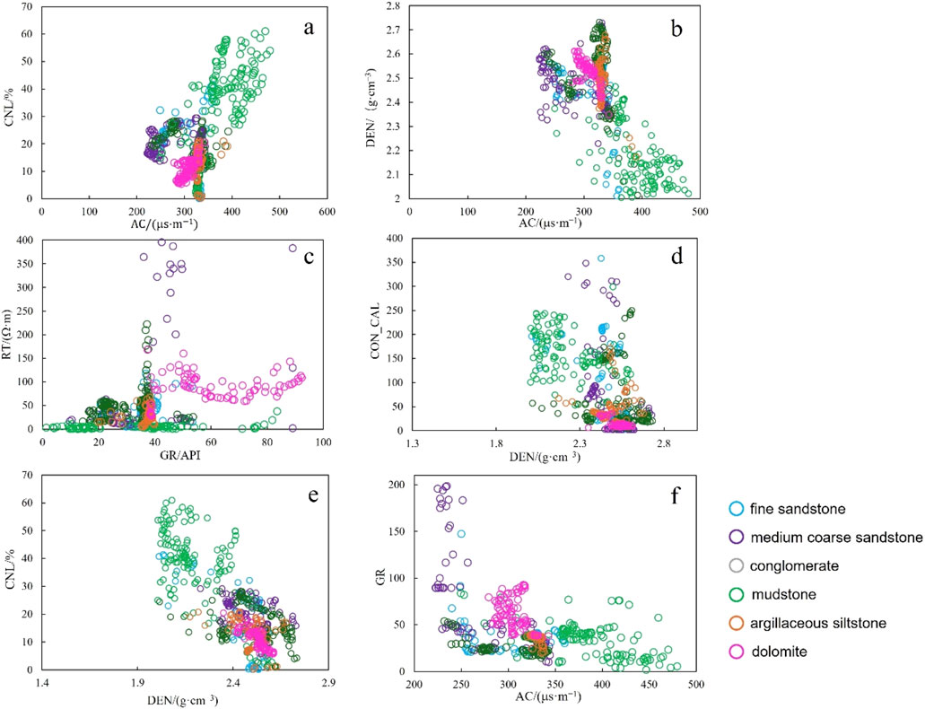
Figure 4. Well logging cross plots of different lithologies. (A) AC-CNL cross plot; (B) AC-DEN cross plot; (C) DEN-CON_CAL cross plot; (D) DEN-CNL cross plot; (E) GR-RT cross plot; (F) AC-GR cross plot.

Figures 4A, B illustrates that the AC-CNL and AC-DEN cross-plots exhibit strong lithological differentiation, whereas the RT-GR and DEN-CON_CAL cross-plots yield moderate results (Figures 4C, D). In contrast, the CNL-DEN and GR-AC cross-plots demonstrate the least effectiveness (Figures 4E, F). Figure 5 indicates that dolomite has a higher GR value and slightly larger neutron response, making it easy to distinguish. The characteristics of mudstone are high GR value, low RT value, high AC value, and low density, with high discrimination. The GR value of fine siltstone shows a medium to low value, with a slightly higher neutron response. The GR value of sandy conglomerate shows a medium to low value, while the CNL value is small.

Figure 5

Figure 5. Logging response characteristics of different lithologies.

2.2 Standardization of logging data

Logging sequence data preprocessing provides near-wellbore stratigraphic information, which can be used to identify changes in stratigraphic interfaces, lithology, and sedimentary environments. However, in practical work, due to measurement errors, noise and outliers, depth migration or missing data, directly using raw logging data for lithology inversion may lead to data mismatch, lack of spatial constraints, low signal-to-noise ratio, and parameter mismatch, which will inevitably affect the accuracy of inversion results (Zheng et al., 2022). Therefore, preprocessing logging curves can improve data quality and availability, eliminate the influence of non-geological factors, and truly reflect stratigraphic characteristics.

The Niuxintuo Oilfield in Liaohe has a long history of development. Over the course of extensive exploration and production activities, systematic errors have emerged in the logging data due to ongoing updates and changes in logging instruments. If the original logging sequence data is directly used for reservoir description, it will affect the accuracy and reliability of the results. Therefore, standardizing logging data can help eliminate systematic errors and enhance the ability to describe, interpret, and predict reservoirs (Zheng et al., 2022).

The key to standardizing logging data is the selection of standard layers, usually selecting mudstones or coal seams with a certain thickness that are stably developed throughout the area. There is a total of seven sets of oil bearing formations in the Niuxintuo oil reservoir. Using GES (Geological Evaluation System) software, the AC, CNL, DEN, GR, RT, and CON_CAL logging curves were standardized in batches.

2.3 Bayes discriminant analysis

Discriminant analysis is a statistical learning method used to establish one or more discriminant functions and assign sample points to different categories (Cui et al., 2023). The goal is to identify features or variables that can distinguish different categories to the greatest extent by analyzing training samples of known categories, and use these features or variables to construct discriminant functions to classify unknown samples.

2.4 Random forest

RF uses Bagging to construct multiple training datasets through self-sampling, and then constructs a base classifier for each sample set, which can improve the overall performance and robustness of the model (Breiman, 2001). Evaluate the contribution of each feature to the model’s predictive performance during classification by calculating the information gain rate of variables. This approach quantifies the importance of each feature parameter, allowing for the selection of variables with higher information gain rates. By focusing on these key variables, the modeling process becomes more streamlined, the influence of redundant features is minimized, and both the model’s performance and its generalization capability are enhanced.

2.5 Support vector machine

SVM is a binary classification model. The basic principle is to construct a hyperplane with maximum spacing in a specific space to achieve correct partitioning of samples of different categories (Wang et al., 2014). For a given training dataset, multiple hyperplanes may satisfy the separation conditions. However, the objective of SVM is to identify the unique hyperplane that maximizes the margin, ensuring the greatest possible separation between classes. Lithology recognition belongs to multi classification problems. For multi classification problems, SVM can adopt one to many (One vs. Rest) or one to one (One vs. One) classification strategies (Wang et al., 2014). In the one-to-many method, each category is combined with other categories to construct multiple binary classification models for classification. In the one-on-one method, a binary classification model is constructed for each pair of categories, and the final result is determined as the category with the highest number of votes through voting or other strategies. Whether it is a binary classification problem or a multi classification problem, SVM can solve it and exhibits good performance in handling high-dimensional data and nonlinear problems.

2.6 Back propagation neural network

BPNN is a multi-layer feedforward neural network trained according to the error backpropagation algorithm (Rumelhart et al., 1986). The learning rule involves using the steepest descent method to iteratively adjust the network’s weights and thresholds through backpropagation, aiming to minimize the network’s total squared error (Dong et al., 2023; Wang and Wang, 2021). The neural network consists of three parts: input layer, hidden layer, and output layer. The main process of BP neural networks is divided into two stages, namely, signal forward propagation and error back propagation. Signal forward propagation refers to the process of transmitting information from the input layer through the hidden layer to the output layer. In contrast, error backpropagation involves transmitting the error from the output layer to the input layer, sequentially adjusting the weights and biases of the hidden-to-output and input-to-hidden layers (Dong et al., 2023; Peng et al., 2024). The main factors affecting the performance of BP neural networks include the number of hidden layer nodes, the selection of activation functions, and the parameter setting of learning rates.

Based on the preprocessing of logging data, we analyze the factors influencing lithology and select the preferred logging response parameters—AC, CNL, DEN, GR, RT, and CON_CAL—as input features for the model. This means the input layer consists of six neurons. The initial number of neurons in the hidden layer is set to 1–2 times the number of input neurons. The optimal number of hidden layer neurons is then determined automatically during the learning process through network structure optimization. The output layer consists of six types of lithology, that is, the number of output layer nodes is six. Basic architecture of a BPNN model is shown in Figure 6.

Figure 6

Figure 6. Basic architecture of a BP neural network.

2.7 Convolutional neural networks

CNN are an important type of artificial neural network, but they are independent of traditional neural networks such as multi-layer perceptual neural networks, RBF neural networks, and fuzzy logic neural networks (Zhong et al., 2019). CNN consists of five layers: data input layer, convolutional computing layer, ReLU excitation layer, pooling layer, and fully connected layer. CNN combines three steps to achieve pattern recognition, including local acceptance domain, weight sharing, and under sampling. The local receptive field refers to the set of units within each layer of the neural network that are connected to the previous layer. Each neuron in this small neighborhood extracts fundamental visual features, such as line segments, endpoints, and angles, from the input data. Weight sharing refers to CNN sharing the weights of some neurons; Therefore, fewer parameters are optimized during the training process. Under sampling can reduce the feature resolution of displacement, amplification, and other forms of distortion invariance (Le and Borji, 2017; Zhong et al., 2019).

3 Results and discussion

3.1 Lithological classification based on bayes discriminant analysis

Binary classification problems are typically addressed using the Fisher criterion, while the Bayes criterion is commonly employed for multi-class classification problems. To tackle the lithology identification of clastic rocks using well logging data, this study develops a discriminant function based on the Bayes criterion. Substitute the logging curve data values for each lithology sample into the following six Bayes discriminant functions to calculate the corresponding function values. Comparing the values of these six functions, which function has the highest value can determine which category the sample is classified into. The coefficients of the Bayesian discriminant function are shown below (Table 2).

Table 2

Table 2. Bayesian discriminant analysis equation coefficients for different lithologies.

According to the Bayes discriminant coefficient table, the Bayes discriminant function can be listed as follows (Equations 1–6):

$\begin{array}{l}\text{Fine\hspace{0.17em}sandstone}=-560.977+1.048\times \text{AC}+2.038\times \text{CNL}+304.246\\ \times \text{DEN}+0.154\times \text{GR}+0.126\times \text{RT}+0.053\\ \times \text{CON}\_\text{CAL}\end{array}(1)$

$\begin{array}{l}\text{Medium\hspace{0.17em}coarse\hspace{0.17em}sandstone}=-576.291+1.050\times \text{AC}+2.129\times \text{CNL}\\ +308.284\times \text{DEN}+0.179\times \text{GR}\\ +0.138\times \text{RT}+0.056\times \text{CO}N\_CAL\end{array}(2)$

$\begin{array}{l}\text{Conglomerate}=-584.414+1.065\times \text{AC}+2.055\times \text{CNL}+311.549\\ \times \text{DEN}+0.141\times \text{GR}+0.127\times \text{RT}\\ +0.053\times \text{CO}N\_CAL\end{array}(3)$

$\begin{array}{l}\text{Mudstone}=-596.900+1.126\times \text{AC}+2.224\times \text{CNL}+304.854\\ \times \text{DEN}+0.198\times \text{GR}+0.128\times \text{RT}+0.057\\ \times \text{CON}\_\text{CAL}\end{array}(4)$

$\begin{array}{l}\text{Transitional\hspace{0.17em}rocks}=-586.249+1.078\times \text{AC}+2.051\times \text{CNL}\\ +310.230\times \text{DEN}+0.174\times \text{GR}+0.121\times \text{RT}\\ +0.052\times \text{CON}\_\text{CAL}\end{array}(5)$

$\begin{array}{l}\text{Dolomite}=-576.476+1.065\times \text{AC}+2.027\times \text{CNL}+307.489\\ \times \text{DEN}+0.206\times \text{GR}+0.123\times \text{RT}+0.05\\ \times \text{CON}\_\text{CAL}\end{array}(6)$

As shown in Table 3, the discriminant coincidence rate was determined by comparing the classification results obtained by substituting the observed lithology values into the discriminant function with the original classifications. The lithology codes are indicated in Table 3 footnote. In this case, the accuracy is 58.2%, indicating that the discriminant analysis method demonstrates limited accuracy in identifying lithology within this study area. The limitations of Bayesian discriminant analysis in lithology identification primarily arise from the following factors. First, the algorithm’s underlying assumptions pose significant challenges: it presumes that the data conforms to a specific probability distribution, typically a normal distribution for different categories. However, real-world lithological data often deviates from this assumption, leading to inaccurate classification outcomes. Additionally, the method assumes that all features are independent, a condition rarely met in practice. In lithological datasets, features frequently exhibit interdependencies, and ignoring these correlations can diminish the model’s accuracy. Furthermore, Bayesian discriminant analysis struggles with handling the inherent complexity of lithological data, limiting its effectiveness in more intricate classification tasks. When addressing complex lithological types, Bayesian discriminant analysis often fails to capture underlying nonlinear relationships, resulting in suboptimal performance under intricate geological conditions.

Table 3

Table 3. Lithology classification result matrix.

3.2 Machine learning methods for lithology recognition

3.2.1 Data preparation

This study used 3,027 sets of logging and core data from 8 core wells in the study area, with 70% of the data for training and 30% for testing. These two datasets each have different functions. The training set is used to create machine learning models and model hyperparameter optimization, while the testing set is used to evaluate the performance of trained machine learning model. The lithological labels of 1–6 correspond to six main lithologies: fine sandstone, medium to coarse sandstone, conglomerate, mudstone, transitional rocks, and dolomite (Table 4).

Table 4

Table 4. Lithology distribution of core samples in the study area.

The following six conventional logging parameters—AC, CNL, DEN, GR, RT, and CON_CAL—are selected as sample attribute values. These parameters form a 7-dimensional vector, comprising six dimensions of parameter values and one dimension for the corresponding lithology label. In machine learning, feature normalization is often essential to eliminate dimensional differences, minimize feature biases, and mitigate the impact of outliers. Normalizing data not only accelerates the training model’s convergence but also facilitates reaching the optimal solution more efficiently. The normalization of logging curves maps the values of the curves to (0,1) through linear transformation. The definition is defined as Equation 7:

$x^{*}=\frac{x-x_{\mathit{min}}}{x_{\mathit{max}}-x_{\mathit{min}}}(7)$

Among them, $x_{\mathit{max}}$ and $x_{\mathit{min}}$ represents the maximum and minimum values in the set of curve values, respectively. Through this processing method, the normalized logging data values will fall within the [0,1] interval, making it easier to compare and analyze.

Exploratory data analysis is performed by creating correlation matrix diagrams to visualize the relationships between different lithologies and logging parameters. Figure 7 presents the correlation matrix diagram illustrating the relationships between various lithologies and logging parameters. The horizontal and vertical axes correspond to six logging parameters, while the diagonal showcases the distribution histograms of different lithologies associated with the parameters on the horizontal axis. Different colors represent various lithologies, and the significant overlap among most logging parameters indicates a lack of clear boundaries, making model classification challenging.

Figure 7

Figure 7. Correlation matrix of different lithology and logging parameters.

3.2.2 Model parameter optimization

To obtain the optimal machine learning model, grid search and 5-fold cross validation methods were used to optimize the hyperparameters of RF, SVM, BPNN, and CNN models (Table 5). The optimization process for the key parameters is illustrated in Figure 8, while unmentioned parameters are set to default values to enhance the model’s accuracy. 5-fold cross-validation provides a reliable estimate of model performance, helps identify optimal parameter settings, and mitigates the risks of overfitting or underfitting. It is widely used for evaluating models and selecting the best parameters, making it suitable for a variety of datasets. The main step of 5-fold cross-validation involves randomly splitting the dataset into five equal parts. Each time, one part is used as the test set, while the remaining four parts serve as the training set. This process is repeated for each part. The optimal parameter combination is then selected based on the highest cross-validation score from the candidate set. After parameter tuning, we optimized the classifier parameters to achieve the best combination (Table 5).

Table 5

Table 5. Optimum parameter values for each model.

Figure 8

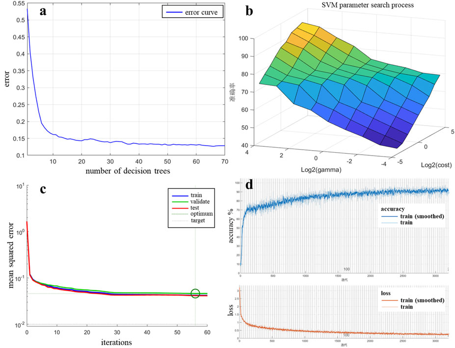
Figure 8. Machine learning algorithms partially hyperparameter optimization. (A) RF decision tree optimization; (B) SVM hyperparameter optimization; (C) BPNN mean square error; (D) CNN Training Progress.

3.3 Comparison of four machine learning lithology methods

3.3.1 Evaluation criterion

The performance of the classification models is evaluated using indicators such as accuracy, precision, recall, and F1-score (Zheng et al., 2022) (Equations 8–11). Accuracy represents the proportion of correct predictions (both positive and negative) out of all predictions. Precision measures the proportion of true positives among the samples predicted as positive. Recall refers to the proportion of correct positive samples among the total actual positives. F1 score is the harmonic average of recall rate and precision rate, which considers the accuracy of the model in predicting positive samples (recall rate) and its recognition ability for positive samples (recall rate). These standard calculation formulas are as follows:

$\text{Accuracy}=\frac{\mathrm{T}P+TN}{\mathrm{T}P+\mathrm{T}N+FP+FN}(8)$

$\text{Precision}=\frac{\mathrm{T}P}{\mathrm{T}P+\mathrm{F}P}(9)$

$\text{Recall}=\frac{\mathrm{T}P}{\mathrm{T}P+\mathrm{F}N}(10)$

$F1-score=2\cdot \frac{Precision\times Recall}{Precision+Recall}(11)$

TP refers to the cases where both the prediction and the actual value are positive. FP refers to the cases where the prediction is positive but the actual value is negative. FN refers to the cases where the prediction is negative but the actual value is positive. TN refers to the cases where both the prediction and the actual value are negative.

3.3.2 Analysis of single point prediction results

After building each machine learning model, the performance of the models is validated and tested. The results are then compared across the four classifiers to evaluate their relative effectiveness (Figure 9). Figure 10 shows the comparison of prediction accuracy results among different models. Among them, SVM has the best classification performance, with a prediction accuracy of 93.87% in the training set and 92.72% in the test set. CNN took second place, with a prediction accuracy of 91.50% for the training set and 90.98% for the test set. The prediction accuracy of the RF training set is 90.33%, and the prediction accuracy of the test set is 89.65%. BPNN has the lowest accuracy, with a prediction accuracy of 86.08% for the training set and 85.01% for the test set. From the above, each machine learning classifier constructed has a high prediction accuracy, with an accuracy rate above 85%. SVM has the best classification performance, with a prediction accuracy rate of up to 93%. The confusion matrices (Figure 11) reveal the misclassification patterns of lithology classes for each model, emphasizing which classes are mistakenly predicted as others. In addition, RF can be used to explain the importance of different parameters in various classification and regression models for model prediction results. The importance ranking of logging parameters for lithology identification based on RF is: GR, AC, RT, CON_ CAL, CNL, DEN (Figure 12).

Figure 9

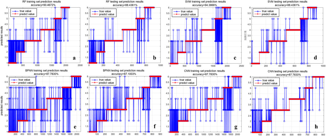
Figure 9. Prediction results of each machine learning classifier. (A) RF training set test results; (B) RF testing set test results; (C) SVM training set test results; (D) SVM testing set test results; (E) BPNN training set test results; (F) BPNN testing set test results; (G) CNN training set test results; (H) CNN testing set test results.

Figure 10

Figure 10. Comparison of prediction accuracy of four machine learning models.

Figure 11

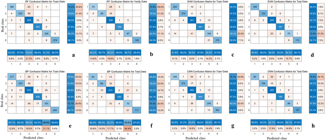
Figure 11. Confusion matrix of each machine learning classifier. (A) RF training set confusion matrix; (B) RF testing set confusion matrix; (C) SVM training set confusion matrix; (D) SVM testing set confusion matrix; (E) BPNN training set confusion matrix; (F) BPNN testing set confusion matrix; (G) CNN training set confusion matrix; (H) CNN testing set confusion matrix.

Figure 12

Figure 12. Analysis of the importance of logging parameters in RF classifier.

The comparison of average precision (Figure 13A) and average F1-score results (Figure 13B) for different models. It can be observed that the BPNN model has the lowest average precision (84.7%) and F1-score (0.84). The RF model ranks second, with an average precision of 91.2% and an F1-score of 0.89. The CNN model achieves a relatively high average accuracy of 92.1%, with an F1-score of 0.91. The SVM model delivers the highest performance, with an average precision of 92.7% and an F1-score of 0.92. In summary, SVM has the best lithology recognition performance, followed by CNN, with both F1-score higher than 0.9, superior to RF and BPNN.

Figure 13

Figure 13. Comparison of lithology identification results of different models. (A) Average prediction accuracy of different models; (B) Average F1-score for different models.

As shown in Table 6, each model demonstrates varying recognition capabilities for different lithology types. SVM showed the highest average F1-score, reaching 0.92. Among them, except for transitional rocks, the F1-score of all other lithologies exceeds 0.92, and the transitional rocks are mainly divided into fine sandstone and medium to coarse sandstone. This could be attributed to the fact that the siltstone class is a non-reservoir in the study area, and the logging response characteristics of fine sandstone and siltstone are quite similar. When classifying lithology, they are classified as transitional rocks, resulting in the lowest prediction accuracy of other models in transitional rocks. The F1-score of CNN and RF is second to SVM, with a high F1-score of 0.96 for both mudstone and dolomite, and the classification of lithology types is relatively similar. The main classification is that fine sandstone and medium to coarse sandstone are divided into conglomerate and transitional rocks are divided into sandy conglomerate and fine sandstone. BPNN also has a high F1-score of 0.91 for both mudstone and dolomite, and the lowest F1-score of 0.64 for transitional rocks. In summary, the SVM classifier demonstrates the best overall performance in lithology identification and is therefore used for lithology prediction in the study area.

Table 6

Table 6. F1-Score for different lithologies using different models.

3.3.3 Lithology prediction in the uncored well

We further validated the effectiveness of the SVM classifier in lithology identification using two blind wells (Figure 14). The results show a high consistency between the lithology predicted by the well-trained SVM model and the lithology observed in the cores, indicating that the well-trained SVM model provides reliable lithology predictions for uncored wells.

Figure 14

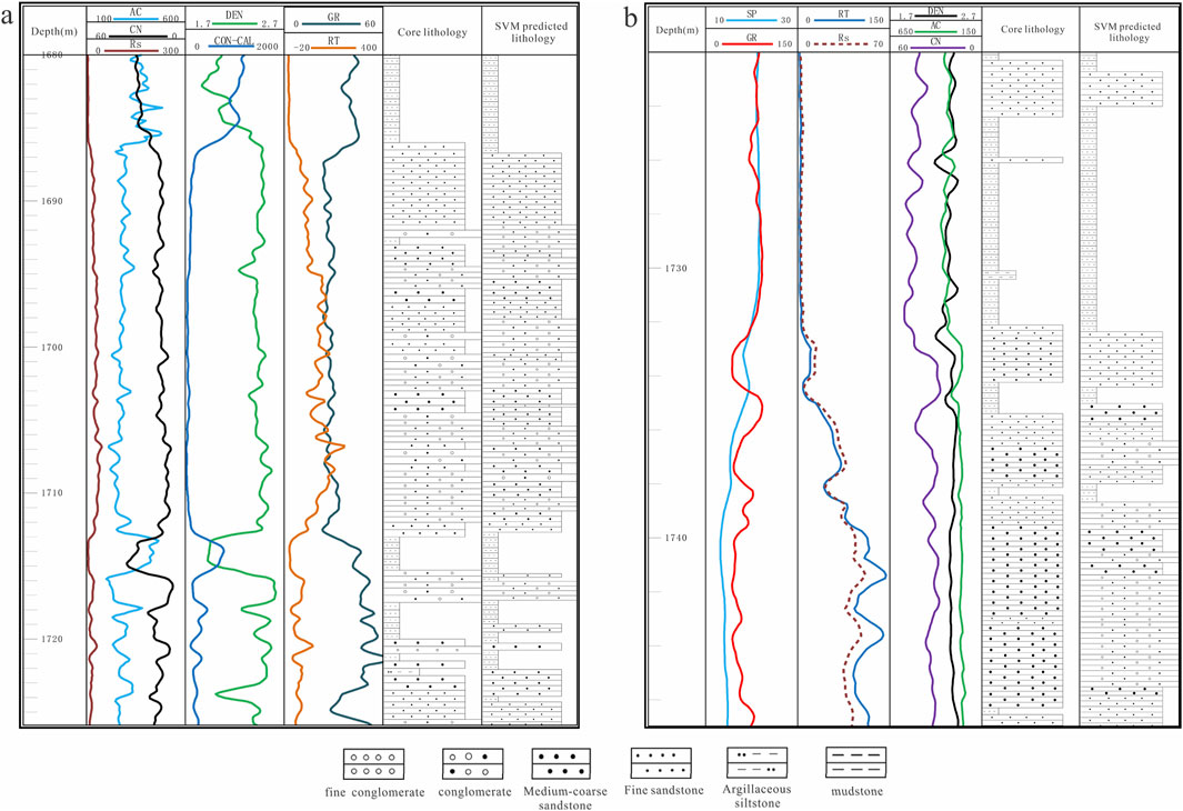
Figure 14. Comparison of core lithology and predicted lithology using well trained SVM classifier. (A) Tuo 31–39 well; (B) Tuo 35–33 well.

4 Conclusion

The main conclusions drawn in this article are as follows:

1. The cross-plot method is not effective in distinguishing lithology, but can help identify sensitive logging curves. The selected sensitive logging curves are: gamma ray (GR), acoustic transmit time (AC), resistivity (RT), conductivity (CON_CAL), compensated neutron (CNL), and density (DEN).

2. Except for Bayes discriminant analysis, all the constructed machine learning classifiers [i.e., Random Forest (RF), Support vector machine (SVM), Back propagation neural network (BPNN), and Convolutional neural networks (CNN)] demonstrate high prediction accuracy, with the accuracy rate exceeding 85%. Among them, SVM classification shows the best performance achieving a prediction accuracy as high as 93%. Blind well tests have confirmed the reliability of the well trained SVM model.

3. RF can be used to explain the importance of different parameters in various classification and regression models for model prediction results. The importance ranking of logging parameters for lithology identification in this study is: GR, AC, RT, CON_ CAL, CNL, DEN.

Data availability statement

The original contributions presented in the study are included in the article/supplementary material, further inquiries can be directed to the corresponding author.

Author contributions

ZF: Conceptualization, Investigation, Methodology, Resources, Writing–original draft, Writing–review and editing. CH: Methodology, Supervision, Writing–original draft. SJ: Methodology, Supervision, and Writing–original draft. ML: Data curation, Formal Analysis, Writing–original draft. YC: Resources, Validation, Writing–original draft. YJ: Investigation, Software, Writing–original draft. YL Data curation, Formal Analysis, Investigation, Writing–review and editing. MT: Investigation, Resources, Writing–original draft.

Funding

The author(s) declare that financial support was received for the research, authorship, and/or publication of this article. The authors declare that this study received funding from CNPC Science and Technology special Project “Research on Greatly Improved Oil recovery Technology in Ultra-high water cut period of medium and high permeability Oilfield” (number: 2023ZZ22). The funder was not involved in the study design, collection, analysis, interpretation of data, the writing of this article, or the decision to submit it for publication.

Conflict of interest

Authors ZF, CH, ML, YC, YJ, YL, and MT were employed by Petrochina Liaohe Oilfield Company.

The remaining author declares that the research was conducted in the absence of any commercial or financial relationships that could be construed as a potential conflict of interest.

Publisher’s note

All claims expressed in this article are solely those of the authors and do not necessarily represent those of their affiliated organizations, or those of the publisher, the editors and the reviewers. Any product that may be evaluated in this article, or claim that may be made by its manufacturer, is not guaranteed or endorsed by the publisher.

References

Amari, S. I. (1993). Backpropagation and stochastic gradient descent method. Neurocomputing 5 (4-5), 185–196. doi:10.1016/0925-2312(93)90006-O

CrossRef Full Text | Google Scholar

Anifowose, F., Abdulraheem, A., and Al-Shuhail, A. (2019). A parametric study of machine learning techniques in petroleum reservoir permeability prediction by integrating seismic attributes and wireline data. J. Petroleum Sci. Eng. 176, 762–774. doi:10.1016/j.petrol.2019.01.110

CrossRef Full Text | Google Scholar

Ashraf, U., Zhang, H., Anees, A., Mangi, H. N., Ali, M., Zhang, X., et al. (2021). A core logging, machine learning and geostatistical modeling interactive approach for subsurface imaging of lenticular geobodies in a clastic depositional system, SE Pakistan. Nat. Resour. Res. 30, 2807–2830. doi:10.1007/s11053-021-09849-x

CrossRef Full Text | Google Scholar

Bhattacharya, S., Carr, T. R., and Pal, M. (2016). Comparison of supervised and unsupervised approaches for mudstone lithofacies classification: case studies from the Bakken and Mahantango-Marcellus Shale, USA. J. Nat. Gas Sci. Eng. 33, 1119–1133. doi:10.1016/j.jngse.2016.04.055

CrossRef Full Text | Google Scholar

Biau, G., and Scornet, E. (2016). A random forest guided tour. Test 25, 197–227. doi:10.1007/s11749-016-0481-7

CrossRef Full Text | Google Scholar

Breiman, L. (2001). Random forests. Mach. Learn. 45, 5–32. doi:10.1023/a:1010933404324

CrossRef Full Text | Google Scholar

Bressan, T. S., de Souza, M. K., Girelli, T. J., and Junior, F. C. (2020). Evaluation of machine learning methods for lithology classification using geophysical data. Comput. and Geosciences 139, 104475. doi:10.1016/j.cageo.2020.104475

CrossRef Full Text | Google Scholar

Chen, T., and Guestrin, C. (2016). “Xgboost: a scalable tree boosting system,” in Proceedings of the 22nd acm sigkdd international conference on knowledge discovery and data mining.

Google Scholar

Cohn, D. A., Ghahramani, Z., and Jordan, M. I. (1996). Active learning with statistical models. J. Artif. Intell. Res. 4, 129–145. doi:10.1613/jair.295

CrossRef Full Text | Google Scholar

Cui, H., Deng, Y., Zhong, R., Li, W., Yu, C., Danyushevsky, L. V., et al. (2023). Determining the ore-forming processes of Dongshengmiao Zn-Pb-Cu deposit: evidence from the linear discriminant analysis of pyrite geochemistry. Ore Geol. Rev. 163, 105782. doi:10.1016/j.oregeorev.2023.105782

CrossRef Full Text | Google Scholar

Delfiner, P., Peyret, O., and Serra, O. (1987). Automatic determination of lithology from well logs. SPE Form. Eval. 2 (03), 303–310. doi:10.2118/13290-PA

CrossRef Full Text | Google Scholar

Dong, S., Wang, Z., and Zeng, L. (2016). Lithology identification using kernel Fisher discriminant analysis with well logs. J. Petroleum Sci. Eng. 143, 95–102. doi:10.1016/j.petrol.2016.02.017

CrossRef Full Text | Google Scholar

Dong, S., Zeng, L., Du, X., He, J., and Sun, F. (2022). Lithofacies identification in carbonate reservoirs by multiple kernel Fisher discriminant analysis using conventional well logs: a case study in A oilfield, Zagros Basin, Iraq. J. Petroleum Sci. Eng. 210, 110081. doi:10.1016/j.petrol.2021.110081

CrossRef Full Text | Google Scholar

Dong, Y., Ma, Z., Xu, F., Su, X., and Chen, F. (2023). Combining the back propagation neural network and particle swarm optimization algorithm for lithological mapping in North China. Remote Sens. 15 (17), 4134. doi:10.3390/rs15174134

CrossRef Full Text | Google Scholar

Ehsan, M., and Gu, H. (2020). An integrated approach for the identification of lithofacies and clay mineralogy through Neuro-Fuzzy, cross plot, and statistical analyses, from well log data. J. Earth Syst. Sci. 129, 101–113. doi:10.1007/s12040-020-1365-5

CrossRef Full Text | Google Scholar

Goodfellow, I., Bengio, Y., and Courville, A. (2016). Deep learning. The MIT Press.

Google Scholar

Helm, H. S., Basu, A., Athreya, A., Park, Y., Vogelstein, J. T., Priebe, C. E., et al. (2023). Distance-based positive and unlabeled learning for ranking. Pattern Recognit. 134, 109085. doi:10.1016/j.patcog.2022.109085

CrossRef Full Text | Google Scholar

Huang, X., Ye, Y., Xiong, L., Lau, R. Y., Jiang, N., and Wang, S. (2016). Time series k-means: a new k-means type smooth subspace clustering for time series data. Inf. Sci. 367, 1–13. doi:10.1016/j.ins.2016.05.040

CrossRef Full Text | Google Scholar

Huang, Y., Liu, Y., Li, C., and Wang, C. (2019). GBRTVis: online analysis of gradient boosting regression tree. J. Vis. 22, 125–140. doi:10.1007/s12650-018-0514-2

CrossRef Full Text | Google Scholar

Jordan, M. I., and Mitchell, T. M. (2015). Machine learning: trends, perspectives, and prospects. Science 349 (6245), 255–260. doi:10.1126/science.aaa8415

PubMed Abstract | CrossRef Full Text | Google Scholar

Kampffmeyer, M., Løkse, S., Bianchi, F. M., Jenssen, R., and Livi, L. (2018). The deep kernelized autoencoder. Appl. Soft Comput. 71, 816–825. doi:10.1016/j.asoc.2018.07.029

CrossRef Full Text | Google Scholar

Le, H., and Borji, A. (2017). What are the receptive, effective receptive, and projective fields of neurons in convolutional neural networks? arXiv Prepr. arXiv 1705.07049. doi:10.48550/arXiv.1705.07049

CrossRef Full Text | Google Scholar

Li, H. (2022). Research progress on evaluation methods and factors influencing shale brittleness: a review. Energy Rep. 8, 4344–4358. doi:10.1016/j.egyr.2022.03.120

CrossRef Full Text | Google Scholar

Li, H., He, S., Radwand, A. E., Xie, J. T., and Qin, Q. R. (2024). Quantitative analysis of pore complexity in lacustrine organic-rich shale and comparison to marine shale: insights from experimental tests and fractal theory. Energy Fuel 38 (17), 16171–16188. doi:10.1021/acs.energyfuels.4c03095

CrossRef Full Text | Google Scholar

Li, H., Zhou, J. L., Mou, X. Y., Guo, H. X., Wang, X. X., An, H. Y., et al. (2022). Pore structure and fractal characteristics of the marine shale of the Longmaxi Formation in the Changning area, southern Sichuan basin, China. Front. Earth Sci. 10, 1018274. doi:10.3389/feart.2022.1018274

CrossRef Full Text | Google Scholar

Lin, J., Li, H., Liu, N., Gao, J., and Li, Z. (2020). Automatic lithology identification by applying LSTM to logging data: a case study in X tight rock reservoirs. IEEE Geoscience Remote Sens. Lett. 18 (8), 1361–1365. doi:10.1109/LGRS.2020.3001282

CrossRef Full Text | Google Scholar

Madani, A., Arnaout, R., Mofrad, M., and Arnaout, R. (2018). Fast and accurate view classification of echocardiograms using deep learning. NPJ Digit. Med. 1 (1), 6. doi:10.1038/s41746-017-0013-1

PubMed Abstract | CrossRef Full Text | Google Scholar

McDowell, G. M., King, A., Lewis, R. E., Clayton, E. A., and Grau, J. A. (1998). “In-site nickel assay by prompt gamma neutron activation wireline logging,” in SEG Annual Meeting (New Orleans, Louisiana: Society of Exploration Geophysicists), 772–775. doi:10.1190/1.1820589

CrossRef Full Text | Google Scholar

Miclea, A. V., Terebes, R., and Meza, S. (2020). “One dimensional convolutional neural networks and local binary patterns for hyperspectral image classification,” in 2020 IEEE International Conference on Automation, Quality and Testing, Robotics (AQTR), Cluj-Napoca, Romania, 21-23 May 2020, 1–6. doi:10.1109/AQTR49680.2020.9129920

CrossRef Full Text | Google Scholar

Miyahara, H., Aihara, K., and Lechner, W. (2020). Quantum expectation-maximization algorithm. Phys. Rev. A 101 (1), 012326. doi:10.1103/PhysRevA.101.012326

CrossRef Full Text | Google Scholar

Peng, Y. Y., Li, Y. F., Yu, H., Han, P. R., Zhu, C., and He, M. C. (2024). Mechanical properties of coal and rock with different dip angles based on true triaxial unloading test. J. Min. Strata Control Eng. 6 (2), 023037. doi:10.13532/j.jmsce.cn10-1638/td.20231222.001

CrossRef Full Text | Google Scholar

Rumelhart, D. E., Hinton, G. E., and Williams, R. J. (1986). Learning representations by back-propagating errors. Nature 323 (6088), 533–536. doi:10.1038/323533a0

CrossRef Full Text | Google Scholar

Sanyal, S. K., Juprasert, S., and Jubasche, J. (1980). An evaluation of a rhyolite-basalt-volcanic ash sequence from well logs. Log. Anal. 21 (1), 3–9.

Google Scholar

Saporetti, C. M., da Fonseca, L. G., Pereira, E., and de Oliveira, L. C. (2018). Machine learning approaches for petrographic classification of carbonate-siliciclastic rocks using well logs and textural information. J. Appl. Geophys. 155, 217–225. doi:10.1016/j.jappgeo.2018.06.012

CrossRef Full Text | Google Scholar

Shan, S. C., Wu, Y. Z., Fu, Y. K., and Zhou, P. H. (2021). Shear mechanical properties of anchored rock mass under impact load. J. Min. Strata Control Eng. 3 (4), 043034. doi:10.13532/j.jmsce.cn10-1638/td.20211014.001

CrossRef Full Text | Google Scholar

Sun, J., Li, Q., Chen, M., Ren, L., Huang, G., Li, C., et al. (2019). Optimization of models for a rapid identification of lithology while drilling-A win-win strategy based on machine learning. J. Petroleum Sci. Eng. 176, 321–341. doi:10.1016/j.petrol.2019.01.006

CrossRef Full Text | Google Scholar

Tian, M., Omre, H., and Xu, H. (2021). Inversion of well logs into lithology classes accounting for spatial dependencies by using hidden markov models and recurrent neural networks. J. Petroleum Sci. Eng. 196, 107598. doi:10.1016/j.petrol.2020.107598

CrossRef Full Text | Google Scholar

Vichi, M., Cavicchia, C., and Groenen, P. J. (2022). Hierarchical means clustering. J. Classif. 39 (3), 553–577. doi:10.1007/s00357-022-09419-7

CrossRef Full Text | Google Scholar

Wang, A. X., Chukova, S. S., and Nguyen, B. P. (2023). Ensemble k-nearest neighbors based on centroid displacement. Inf. Sci. 629, 313–323. doi:10.1016/j.ins.2023.02.004

CrossRef Full Text | Google Scholar

Wang, G., Carr, T. R., Ju, Y., and Li, C. (2014). Identifying organic-rich Marcellus Shale lithofacies by support vector machine classifier in the Appalachian basin. Comput. and Geosciences 64, 52–60. doi:10.1016/j.cageo.2013.12.002

CrossRef Full Text | Google Scholar

Wang, J., and Wang, X. L. (2021). Seepage characteristic and fracture development of protected seam caused by mining protecting strata. J. Min. Strata Control Eng. 3 (3), 033511. doi:10.13532/j.jmsce.cn10-1638/td.20201215.001

CrossRef Full Text | Google Scholar

Wang, P., Chen, X., Wang, B., Li, J., and Dai, H. (2020). An improved method for lithology identification based on a hidden Markov model and random forests. Geophysics 85 (6), IM27–IM36. doi:10.1190/geo2020-0108.1

CrossRef Full Text | Google Scholar

Xu, H., Li, L., and Guo, P. (2021a). Semi-supervised active learning algorithm for SVMs based on QBC and tri-training. J. Ambient Intell. Humaniz. Comput. 12, 8809–8822. doi:10.1007/s12652-020-02665-w

CrossRef Full Text | Google Scholar

Xu, Z., Ma, W., Lin, P., Shi, H., Pan, D., and Liu, T. (2021b). Deep learning of rock images for intelligent lithology identification. Comput. and Geosciences 154, 104799. doi:10.1016/j.cageo.2021.104799

CrossRef Full Text | Google Scholar

Yan, T., Xu, R., Sun, S. H., Hou, Z. K., and Feng, J. Y. (2024). A real-time intelligent lithology identification method based on a dynamic felling strategy weighted random forest algorithm. Petroleum Sci. 21 (2), 1135–1148. doi:10.1016/j.petsci.2023.09.011

CrossRef Full Text | Google Scholar

Yang, Z., and Xu, Y. (2018). A safe screening rule for Laplacian support vector machine. Eng. Appl. Artif. Intell. 67, 309–316. doi:10.1016/j.engappai.2017.10.011

CrossRef Full Text | Google Scholar

Zhang, X., Wen, J., Sun, Q., Wang, Z., Zhang, L., and Liang, P. (2023). Lithology identification technology of logging data based on deep learning model. Earth Sci. Inf. 16 (3), 2545–2557. doi:10.1007/s12145-023-01051-2

CrossRef Full Text | Google Scholar

Zheng, D., Hou, M., Chen, A., Zhong, H., Qi, Z., Ren, Q., et al. (2022). Application of machine learning in the identification of fluvial-lacustrine lithofacies from well logs: a case study from Sichuan Basin, China. J. Petroleum Sci. Eng. 215, 110610. doi:10.1016/j.petrol.2022.110610

CrossRef Full Text | Google Scholar

Zhong, Z., Carr, T. R., Wu, X., and Wang, G. (2019). Application of a convolutional neural network in permeability prediction: a case study in the Jacksonburg-Stringtown oil field, West Virginia, USA. Geophysics 84 (6), B363–B373. doi:10.1190/geo2018-0588.1

CrossRef Full Text | Google Scholar

Zhou, K., Zhang, J., Ren, Y., Huang, Z., and Zhao, L. (2020). A gradient boosting decision tree algorithm combining synthetic minority oversampling technique for lithology identification. Geophysics 85 (4), WA147–WA158. doi:10.1190/geo2019-0429.1

CrossRef Full Text | Google Scholar

Zhou, X. (2022). Reservoir characteristics and main controlling factors of the fourth member of shahejie formation in Niuxintuo area of western Liaohe sag. Special Oil and Gas Reservoirs 29 (5), 49. (in Chinese with an English abstract). doi:10.3969/j.issn.1006-6535.2022.05.007

CrossRef Full Text | Google Scholar