Stochastic inversion method based on compressed sensing frequency division waveform indication prior

The stochastic inversion method using logging data as conditional data and seismic data as constraint data has a higher vertical resolution than the conventional deterministic inversion method. However, it remains challenging to reduce the randomness of the prior obtained through conventional random simulation techniques and to enhance its accuracy. To address this, we propose a stochastic inversion method based on compressed sensing frequency-division waveform indication prior. This method fully considers the geophysical mapping relationship between the observed seismic data and the parameters to be inverted across different frequency bands. And the correlation coefficients between the seismic data at the known points and the predicted points are obtained by solving the low-rank system of equations through the compressed sensing method. Consequently, pseudo-kriging simulation of well data is performed based on the similarity between known and predicted seismic waveforms, thus establishing prior information indicated by the seismic waveforms. On this basis, the stochastic inversion results are solved using a very fast simulated annealing method. Both model calculations and field data inversion effects demonstrate that the compressed sensing frequency-division waveform indication method effectively improves the accuracy of solving prior information under a low-rank matrix. Ultimately, the proposed stochastic inversion method based on compressed sensing frequency division waveform indication prior enhances the inversion accuracy and provides advantages in identifying underground oil and gas reservoirs.

Introduction

Seismic waveforms are the most intuitive display of seismic signals and contain a wealth of information. Early research on seismic waveforms primarily focused on classifying waveforms for seismic phase analysis using various similarity calculation methods. Gao (2013) analyzed the seismic waveform characteristics of wells in different types of reservoirs, established corresponding waveform databases, and explored comparison methods for waveform structures. Zhou (2015) quantitatively described the seismic waveform by normalizing the seismic waveform correlation coefficient, compared the “unknown waveform” with the “known waveform” from a waveform library to predict the distribution of high-quality oil and gas reservoirs. Zhang et al. (2016) implemented seismic waveform classification and seismic phase identification using supervised artificial neural networks. Cai et al. (2018) introduced a semi-supervised K-means algorithm for distance measurements, combing it with a semi-supervised dimensionality reduction algorithm to classify waveform and generate seismic phase diagrams. Song et al. (2022) proposed a dynamic sub-window matching method to measure the similarity between waveforms of varying lengths, thereby achieving seismic waveform classification. And then, Lu et al. (2019) established the correspondence between reservoir fluid types and seismic waveforms by applying the fast weight k-nearest neighbor algorithm to waveform classification, thus realizing the identification of slit-hole type reservoir fluids. Zhang et al. (2020) combined continuous wavelet transform and convolutional neural networks to develop a new waveform classifier. From the perspective of seismic phase analysis, Xu et al. (2022) compared the accuracy of reservoir prediction results obtained via conventional seismic waveform classification method and seismic texture attribute clustering. Their findings demonstrated that seismic texture attribute clustering provides more reliable waveform classification results. At the same time, a group of scholars have achieved reservoir prediction by directly classifying seismic waveforms.

After that, researchers began extending the classification of seismic waveforms to the inversion field, leveraging the similarities in seismic waveform features. Gao et al. (2017) proposed a seismic waveform indication inversion method based on seismic data, integrating sedimentary laws and seismic geology to extract common information from logging curves when the depositional environments are similar. This process fully embodies the phase control concept and improves the computational efficiency and prediction accuracy compared with traditional methods. Subsequently, Chen et al. (2020) systematically expounded the principle of seismic waveform indication inversion and implemented it by establishing a mapping relationship between seismic waveform structures and high-frequency logging curve structures. Gu et al. (2021) utilized a preferred waveform similarity method, considering AVO feature similarity and spatial distances correlations between seismic trace sets, to achieve waveform-driven multiparameter constrained high-resolution inversion. Building on phase control, Shi S. Z et al. (2024) used the connection between seismic waveforms and logging curves for vertical mapping, integrating waveform indication inversion to characterize lithological combinations in coal-bearing strata and distinguish between sandstone and mudstone. Seismic waveforms contain a variety of information on seismic kinematics and dynamics, which are a comprehensive response to a variety of geologic information such as geologic depositional effects, lithologic facies combinations, reservoir properties, and fluids. Changes in seismic waveforms reflect variations in lithologic combinations, as similar sedimentary features often correspond to similar lithologic assemblages, which in turn produce comparable seismic waveform characteristics. Therefore, seismic waveform indication inversion is a viable approach for identifying underground reservoirs. The key challenge lies in establishing the intrinsic connection between seismic waveforms and high-frequency logging information. To address this, when establishing prior information, this paper establishes prior information by dividing the frequency bands, and then integrates the prior information of different frequency bands into the prior information of the entire frequency band for inversion.

Studies by different scholars have demonstrated the applicability of waveform indication methods in a priori information building and inversion. However, the accuracy of prior information derived from seismic waveforms depends critically on the precision of the correlation coefficient calculations. This is particularly true for low-rank matrices, where the accuracy of solving them needs further improvement. Yu et al. (2024) addressed the challenge of solving large sparse matrices by introducing an innovative dimensionality reduction strategy based on the discrete cosine transform, which reduces the problem to solving smaller matrices. Similarly, Shi Y et al. (2024) employed a fast multi- Gaussian inversion method to reduce the dimensionality of the core inverse matrix, significantly alleviating the difficulties associated with solving large matrix inverses in Bayesian linearized inversion. These studies on large matrix solutions have also provided valuable insights for this paper.

In addition, scholars have conducted extensive research on inversion algorithms. Metropolis et al. (1953) first proposed the concept of simulated annealing. Kirkpatrick et al. (1983) used simulated annealing to find the optimal solution to the combinatorial problem. Basu and Frazer. (1990) enhanced the simulated annealing algorithm by incorporating the temperature-dependent Cauchy or Cauchy model to generate new solutions. Mosegaard and Vestergaard (1991) introduced the simulated annealing method into seismic inversion and solved the seismic trace inversion problem through global random optimization. Srivastava and Sen (2009) employed a nonlinear optimization method using fast simulated annealing to achieve optimal inversion results by minimizing the objective function. Wang et al. (2021) solved the inversion problem of elastic impedance based on a very fast simulated annealing method, which effectively improves the inversion efficiency. Scholars have also explored improvements to simulated annealing, such as fast quantum annealing methods, which further enhance computational efficiency (Zhao et al., 2018). Based on previous research, this paper uses a relatively mature very fast simulated annealing method to solve the inverse problem.

Compressed sensing frequency division waveform indication modeling method

Changes in seismic amplitude indirectly reflect the spatial variation of underground reservoir parameters. Since there exists a certain geophysical mapping relationship between observed seismic data and reservoir parameters (Li et al., 2022), the interpolation of unknown reservoir parameters in the subsurface can be completed by guiding known well information based on known observed seismic data. The stochastic inversion method based on compressed sensing frequency-division waveform indication prior draws on the traditional geostatistical prior information construction method. The core approach for building a priori information using seismic waveform indication is as follows. The first point is to collect statistics on the well-side seismic trace data of all wells and the prediction parameter curves on the wells based on the data of all wells in the work area. The second point is to solve the low-rank equation group through the compressed sensing method to obtain the correlation coefficient between the seismic waveform at the point to be predicted and the seismic waveform at all sample points of the well-side seismic trace. The third point is the unbiased optimal estimation of well data with high-frequency components using pseudo-Kriging interpolation methods. The final inverted seismic waveforms are adjusted to match the original seismic characteristics, including the more deterministic high-frequency elastic parameters.

Waveform indication modeling is based on the geophysical mapping relationship between observed seismic data and parameters to be inverted, utilizing the similarity of seismic waveforms to simulate unknown underground model parameters from selected well samples. Zhou et al. (2021) described the modeling process of the parameters to be inverted using the ordinary pseudo-Kriging interpolation formula:

$Z\left(x_0\right)={\displaystyle \sum _{i=1}^n}{\lambda }_{i}Z\left(x_i\right)(1)$

where, $Z\left(x_0\right)$ is the value at the interpolation parameter $x_0$ to be simulated. $Z\left(x_i\right)$ is the corresponding value at the predicted well sample point $x_i$ selected by the well-side seismic data. ${\lambda }_i$ is the weight of $Z\left(x_i\right)$ at the point to be interpolated. $n$ is the number of participating wells.

Assume that the expected $c$ and variance ${\sigma }^2$ for any point $p\left(x,y\right)$ in a region are the same, and for any point $p\left(x,y\right)$, we have:

$E\left[p\left(x,y\right)\right]=E\left(p\right)=c$

$\Delta \left[p\left(x,y\right)\right]={\sigma }^2$

The unbiased estimation condition is:

$E\left({\widehat{z}}_0-z_0\right)=0(2)$

The ordinary Kriging interpolation formula is:

${\widehat{z}}_0={\displaystyle \sum _{i=1}^n}{\lambda }_i{z}_i(3)$

where, $z_0$ is the seismic data at the point to be predicted. ${\widehat{z}}_0$ is the seismic data at the point to be predicted after Kriging interpolation. $z_i$ is the seismic data at known points. Substituting Equation 3 into Equation 2, there is:

$E\left({\displaystyle \sum _{i=1}^n}{\lambda }_i{z}_i-z_0\right)=0$

${\displaystyle \sum _{i=1}^n}{\lambda }_i=1$

The estimated variance is:

$J=\Delta \left({\widehat{z}}_0-z_0\right)={\displaystyle \sum _{i=1}^n}{\displaystyle \sum _{j=0}^n}{\lambda }_i{\lambda }_j\text{Cov}\left(z_i,z_j\right)-2{\displaystyle \sum _{i=1}^n}{\lambda }_i\text{Cov}\left(z_i,z_0\right)+{\sigma }^2$

Let $C_{ij}=\text{Cov}\left(z_i,z_j\right)$, then we have:

$J={\displaystyle \sum _{i=1}^n}{\displaystyle \sum _{j=0}^n}{\lambda }_i{\lambda }_j{C}_{ij}-2{\displaystyle \sum _{i=1}^n}{\lambda }_i{C}_{i0}+{\sigma }^2(4)$

The correlation coefficient is:

$r_{ij}=\frac{C_{ij}}{\sqrt{\Delta \left(z_i\right)}\sqrt{\Delta \left(z_j\right)}}(5)$

where, $r_{ij}$ is the correlation coefficient between the seismic waveform of seismic data point $z_i$ and the seismic waveform of seismic data point $z_j$.Substituting Equation 5 into Equation 4, we have:

$\begin{array}{l}J={\displaystyle \sum _{i=1}^n}{\displaystyle \sum _{j=0}^n}{\lambda }_i{\lambda }_j{r}_{ij}\sqrt{\Delta \left(z_i\right)}\sqrt{\Delta \left(z_j\right)}-2{\displaystyle \sum _{i=1}^n}{\lambda }_i{r}_{i0}\sqrt{\Delta \left(z_i\right)}\sqrt{\Delta \left(z_0\right)}+{\sigma }^2\\ ={\displaystyle \sum _{i=1}^n}{\displaystyle \sum _{j=0}^n}{\lambda }_i{\lambda }_j{r}_{ij}{\sigma }^2-2{\displaystyle \sum _{i=1}^n}{\lambda }_i{r}_{i0}{\sigma }^2+{\sigma }^2\end{array}$

Our goal is to find the set of ${\lambda }_i$ that minimizes $J$, and $J$ is a function of ${\lambda }_i$. Therefore, the partial derivative of $J$ with respect to ${\lambda }_i$ is calculated and set to 0, that is:

$\frac{\mathrm{\partial }J}{\mathrm{\partial }{\lambda }_i}=0$

The optimal ${\lambda }_i$ obtained from the solution needs to satisfy the ${\displaystyle \sum _{i=1}^n}{\lambda }_i=1$. Therefore, the new objective function can be reconstructed:

$W=J+2\varphi \left({\displaystyle \sum _{i=1}^n}{\lambda }_i-1\right)$

We solve the optimization problem through the above formula. Where $\varphi$ is the Lagrange multiplier. Solving the minimum parameter set $\varphi$ and ${\lambda }_1,{\lambda }_2,\cdots ,{\lambda }_n$ of $W$, we can get the minimized $J$ under the ${\displaystyle \sum _{i=1}^n}{\lambda }_i=1$ constraint, that is:

$\left\{\begin{array}{l}\frac{\mathrm{\partial }\left[J+2\varphi \left({\displaystyle \sum _{i=1}^n}{\lambda }_i-1\right)\right]}{\mathrm{\partial }{\lambda }_k}=0k=1,2,\cdots ,n\\ \frac{\mathrm{\partial }\left[J+2\varphi \left({\displaystyle \sum _{i=1}^n}{\lambda }_i-1\right)\right]}{\mathrm{\partial }\varphi }=0\end{array}\right.$

$\left\{\begin{array}{l}\frac{\mathrm{\partial }\left[{\displaystyle \sum _{i=1}^n}{\displaystyle \sum _{j=0}^n}{\lambda }_i{\lambda }_j{r}_{ij}{\sigma }^2-2{\displaystyle \sum _{i=1}^n}{\lambda }_i{r}_{i0}{\sigma }^2+{\sigma }^2+2\varphi \left({\displaystyle \sum _{i=1}^n}{\lambda }_i-1\right)\right]}{\mathrm{\partial }{\lambda }_k}=0\\ \frac{\mathrm{\partial }\left[{\displaystyle \sum _{i=1}^n}{\displaystyle \sum _{j=0}^n}{\lambda }_i{\lambda }_j{r}_{ij}{\sigma }^2-2{\displaystyle \sum _{i=1}^n}{\lambda }_i{r}_{i0}{\sigma }^2+{\sigma }^2+2\varphi \left({\displaystyle \sum _{i=1}^n}{\lambda }_i-1\right)\right]}{\mathrm{\partial }\varphi }=0\end{array}\right.\Rightarrow$

$\left\{\begin{array}{l}{\displaystyle \sum _{j=1}^n}{\lambda }_j\left(r_{kj}+r_{jk}\right){\sigma }^2-2r_{k0}{\sigma }^2+2\varphi =0\\ {\displaystyle \sum _{i=1}^n}{\lambda }_i=1\end{array}\right.(6)$

Due to $r_{kj}=r_{jk}$, Then Equation 6 becomes:

$\left\{\begin{array}{l}{\displaystyle \sum _{j=1}^n}{\lambda }_j{r}_{kj}-r_{k0}+\frac{\varphi }{{\sigma }^2}=0k=1,2,\cdots ,n\\ {\displaystyle \sum _{i=1}^n}{\lambda }_i=1\end{array}\right.(7)$

From Equation 7, we can get the equation group for solving the weight coefficient:

$\left\{\begin{array}{l}{r}_{11}{\lambda }_1+r_{12}{\lambda }_2+\cdots +r_{1n}{\lambda }_n+\frac{\varphi }{{\sigma }^2}=r_{10}\\ r_{21}{\lambda }_1+r_{22}{\lambda }_2+\cdots +r_{2n}{\lambda }_n+\frac{\varphi }{{\sigma }^2}=r_{20}\\ ⋮\\ r_{n1}{\lambda }_1+r_{n2}{\lambda }_2+\cdots +r_{nn}{\lambda }_n+\frac{\varphi }{{\sigma }^2}=r_{n0}\end{array}\right.$

Written in matrix form:

$\left(\begin{array}{ccccc}{r}_{11}& r_{12}& \cdots & r_{1n}& 1\\ r_{21}& r_{22}& \cdots & r_{2n}& 1\\ & & ⋮& & \\ r_{n1}& r_{n2}& \cdots & r_{nn}& 1\\ 1& 1& \cdots & 1& 0\end{array}\right)\left(\begin{array}{l}{\lambda }_1\\ {\lambda }_2\\ ⋮\\ {\lambda }_n\\ \frac{\varphi }{{\sigma }^2}\end{array}\right)=\left(\begin{array}{l}{r}_{10}\\ r_{20}\\ ⋮\\ r_{n0}\\ 1\end{array}\right)(8)$

By performing an inverse operation on the matrix, the weight of the seismic data at the known point at the point to be predicted can be obtained. According to the geophysical mapping relationship between the observed seismic data and the parameters to be inverted, the weight ${\lambda }_j$ obtained from this matrix replaces ${\lambda }_i$ in Equation 1, thereby completing the establishment of the initial model.

Seismic reflections from reservoirs of varying thicknesses correspond to specific dominant frequencies in the frequency domain. Generally, high-frequency tuning energy reflects the tuning response of thin layers, while low-frequency energy corresponds to the tuning response of thick layers. The tuning response of the wavelet varies with reservoir thicknesses, as geological bodies of different thicknesses are associated with distinct dominant frequencies. Therefore, when modeling waveform indication, we first model by dividing the frequency bands and establish elastic parameter models under different frequency bands. These models in different frequency bands are integrated in the frequency domain to obtain the final required elastic parameter model.

Next, we simplify Equation 8, let $A=\left(\begin{array}{ccccc}{r}_{11}& r_{12}& \cdots & r_{1n}& 1\\ r_{21}& r_{22}& \cdots & r_{2n}& 1\\ & & ⋮& & \\ r_{n1}& r_{n2}& \cdots & r_{nn}& 1\\ 1& 1& \cdots & 1& 0\end{array}\right)$, $x=\left(\begin{array}{l}{\lambda }_1\\ {\lambda }_2\\ ⋮\\ {\lambda }_n\\ \frac{\varphi }{{\sigma }^2}\end{array}\right)$, $b=\left(\begin{array}{l}{r}_{10}\\ r_{20}\\ ⋮\\ r_{n0}\\ 1\end{array}\right)$. Then Equation 8 can be written as:

$Ax=b$

However, when obtaining the matrix $x$ containing weight coefficients, $A$ is a matrix with insufficient rank and very small rank. It is extremely unstable when performing the inverse operation, resulting in the obtained matrix $x$ containing the weight coefficients being inaccurate and unstable. As a result, when modeling waveform indications, the modeling results deviate significantly from the real data and the modeling results are inaccurate. To address these modeling discrepancies caused by an unreliable weight coefficient matrix, we apply the compressed sensing method to obtain the weight coefficient matrix. L1 regularized linear regression is expressed as follows (Chen et al., 2022):

$l\left(x\right)=\left(1/2\right)\parallel Ax-b{\parallel }_2^2(9)$

When we solve Equation 9, we are also solving the following equation:

$\text{minimize\hspace{0.17em}}\left(1/2\right)\parallel Ax-b{\parallel }_2^2+\lambda \parallel x{\parallel }_1$

At this point, we introduce the alternating direction method of multipliers to solve:

$\left\{\begin{array}{l}\text{minimize\hspace{0.5em}}f\left(x\right)+g\left(z\right)\\ \text{subject\hspace{0.17em}to\hspace{0.5em}}x-z=0\end{array}\right.(10)$

where, $f\left(x\right)=\left(1/2\right)\parallel Ax-b{\parallel }_2^2$, $g\left(z\right)=\lambda \parallel z{\parallel }_1$. Based on Equation 9 to Equation 10, we can derive:

$\begin{array}{l}{x}^{k+1}=\arg {\min }_x\left(1/2\right)\parallel Ax-b{\parallel }_2^2+\frac{\rho }{2}{‖x-z^{\left(k\right)}+u^{\left(k\right)}‖}_2^2{z}^{\left(k+1\right)}\\ =\arg {\min }_z\lambda \parallel z{\parallel }_1+\frac{\rho }{2}{‖x^k-z+u^{\left(k\right)}‖}_2^2{u}^{\left(k+1\right)}\\ =u^{\left(k\right)}+x^k-z^{\left(k\right)}\end{array}$

Derivation to zero for $x$ update:

$\begin{array}{l}{A}^T\left(Ax-b\right)+\rho \left(x-z^k+u^k\right)=0\\ \left(A^{T}A+\rho I\right)x-\left(A^{T}b+\rho \left(z^k-u^k\right)\right)=0\\ x^{k+1}={\left(A^{T}A+\rho I\right)}^{-1}\left(A^{T}b+\rho \left(z^k-u^k\right)\right)\end{array}$

A soft thresholding is introduced to constrain the update of $z$:

$\begin{array}{l}{x}^{k+1}:={\left(A^{T}A+\rho I\right)}^{-1}\left(A^{T}b+\rho \left(z^k-u^k\right)\right)\\ z^{k+1}:=S_{\lambda /\rho }\left(x^{k+1}+u^k\right)\\ u^{k+1}:=u^k+x^{k+1}-z^{k+1}\end{array}$

Here $A^{T}A+\rho I$ is always reversible and since $\rho >0$. $S$ is the soft threshold operator with the following formula:

$S_{\lambda /\rho }\left(x^{k+1}+u^k\right)=\left\{\begin{array}{l}{x}^{k+1}+u^k-\lambda /\rho ,x^{k+1}+u^k>\lambda /\rho \\ 0,\left|x^{k+1}+u^k\right|⩽\lambda /\rho \\ x^{k+1}+u^k+\lambda /\rho ,x^{k+1}+u^k<-\lambda /\rho \end{array}\right.$

Therefore, a more accurate weight coefficient matrix can be obtained by using the aforementioned compressed sensing method, resulting in more reliable prior information.

Numerical example

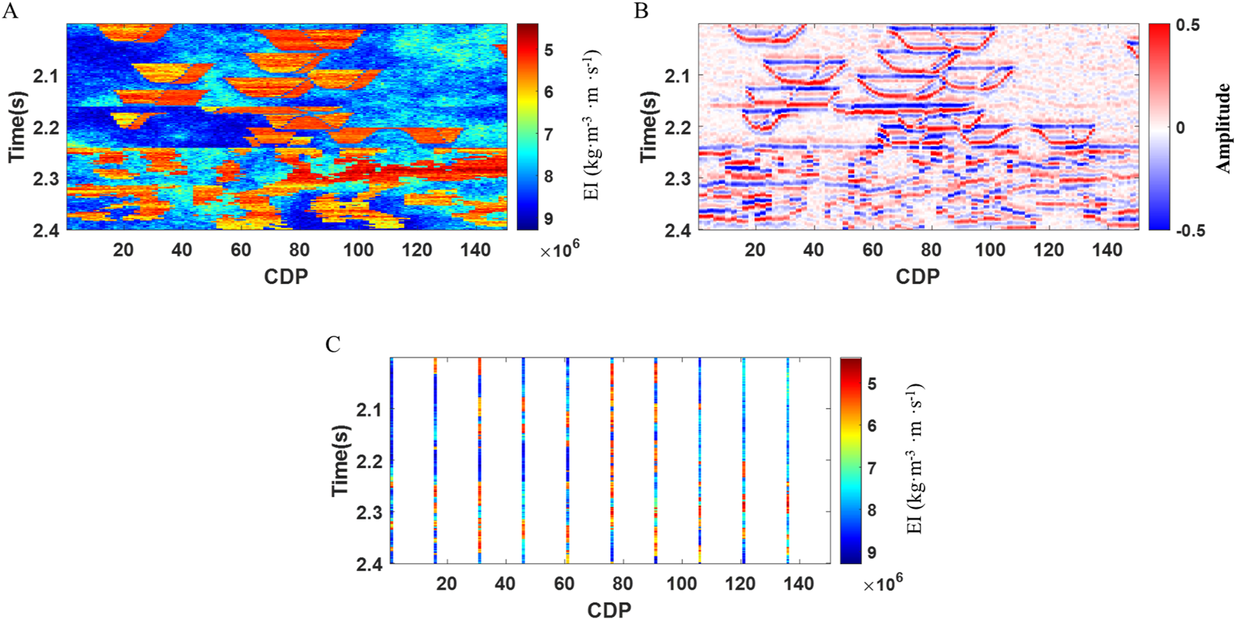
To validate the effectiveness of the method in this paper, the marmousi2 partial model is selected for testing. We take near angle elastic impedance as an example for simulation. Figure 1 presents the small-angle elastic impedance model data (Figure 1A), the corresponding synthetic seismic data (Figure 1B), and the extracted pseudo-well data. The pseudo-well data include one pseudo-well (Figure 1C), three pseudo-wells (Figure 1D), and five pseudo-wells (Figure 1E). Figure 2 shows the Kriging simulation results (Figures 2A, C, E) and the simulation results (Figures 2B, D, F) of this paper’s method obtained using one pseudo-well, three pseudo-wells, and five pseudo-wells, respectively. The red arrows indicate the locations of oil-bearing reservoirs in the model data. From the figures, it is evident that the simulation results improve as the number of pseudo-wells increases, for both the Kriging method and the method proposed in this paper. In the case of fewer pseudo-wells, the Kriging method fails to capture the spatial variation of the elastic parameters. However, even with a small number of pseudo wells, the method in this paper is still able to effectively utilize the seismic waveform information, leading to a more accurate simulation of elastic parameters at oil-bearing locations. Moreover, the simulated small-angle elastic impedance follows the trend of the seismic waveform, which aligns with the spatial structural characteristics of the underground medium. The relative errors of Kriging’s method are 0.25, 0.24, and 0.22 for the simulation results of the oil-bearing layers at the red arrows under one pseudo-well, three pseudo-wells, and five pseudo-wells, respectively. For the method proposed in this paper, the relative errors are 0.21, 0.14, and 0.10, respectively. These results demonstrate that the method in this paper yields relatively smaller relative errors in comparison to the Kriging method.

Figure 1

Figure 1. Near angle elastic impedance model, synthetic seismic data, and different pseudo-well data. (A) Near angle elastic impedance model data, (B) Near angle synthetic seismic data, (C) 1 pseudo-well extracted, (D) 3 pseudo-wells extracted, (E) 5 pseudo-wells extracted.

Figure 2

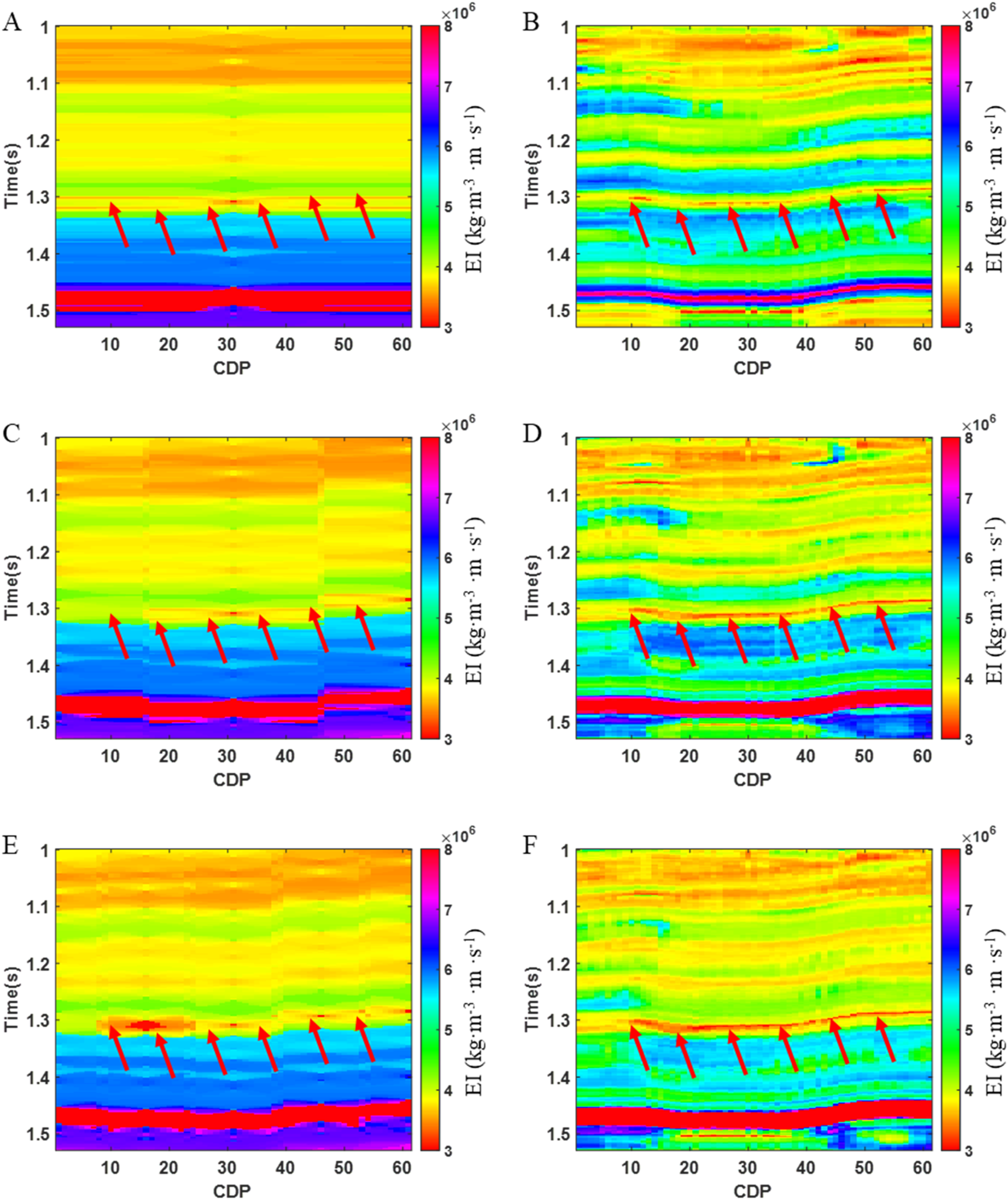
Figure 2. Kriging simulation results of different pseudo wells and simulation results of this paper’s method. (A) Kriging simulation results for 1 pseudo-well, (B) Simulation results of this paper’s method for 1 pseudo-well, (C) Kriging simulation results for 3 pseudo-wells, (D) Simulation results of this paper’s method for 3 pseudo-wells, (E) Kriging simulation results for 5 pseudo-wells, (F) Simulation results of this paper’s method for 5 pseudo-wells.

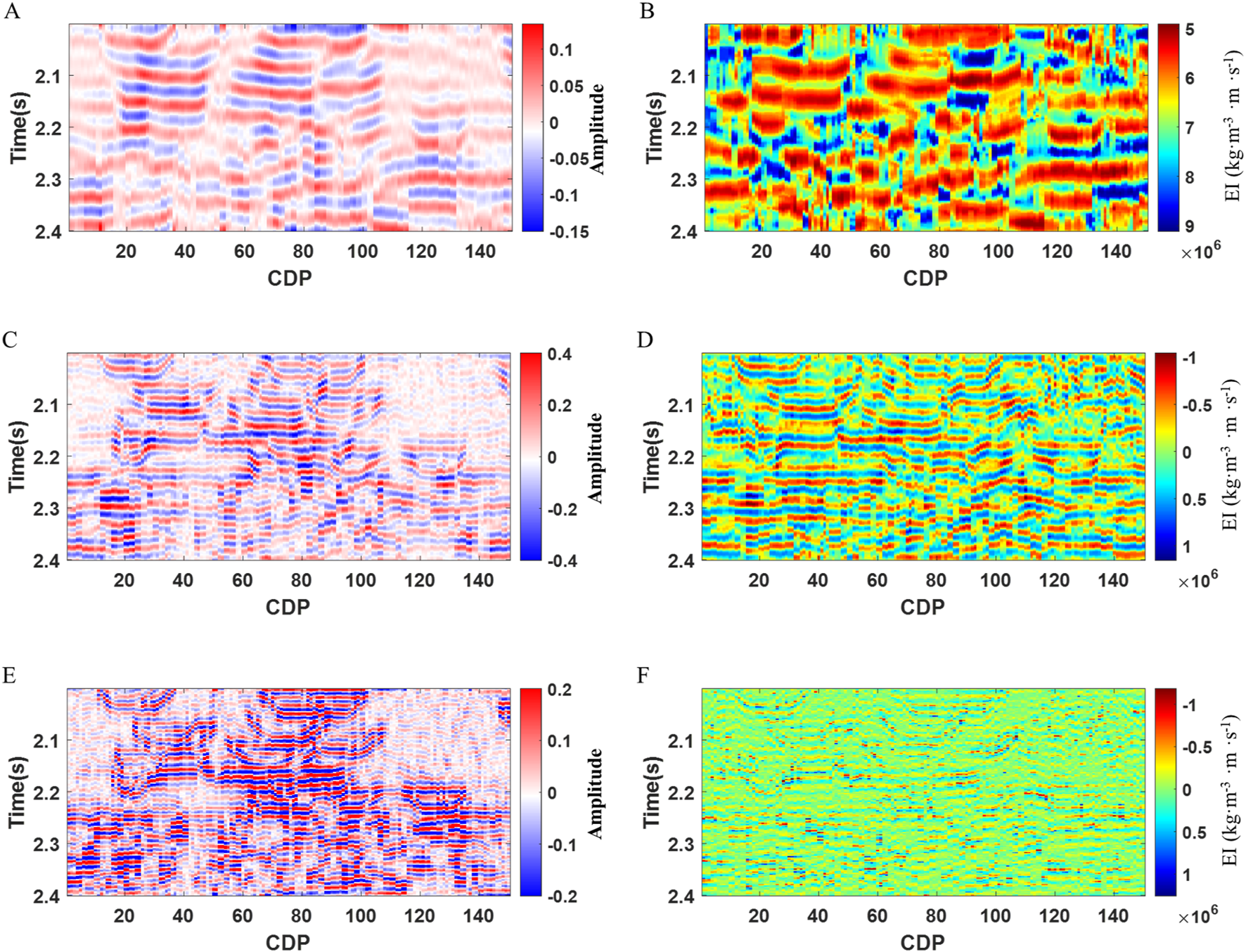
Based on the above method, the modeling effect of the compressed sensing frequency division waveform indication modeling method is further tested by taking the small-angle elastic impedance model data and synthetic seismic data as examples. We set the low frequency range to 0–20Hz, the medium frequency range to 20–45Hz, and the frequency greater than 45Hz as the high frequency range. Figure 3 presents the seismic data corresponding to the near-angle seismic data for the low-frequency (Figure 3A), medium-frequency (Figure 3C), and high-frequency (Figure 3E) bands, along with the simulation results for the near-angle elastic impedance in these frequency bands: the low-frequency (Figure 3B), medium-frequency (Figure 3D), and high-frequency (Figure 3F). As shown in the figure, the elastic impedance simulation results of different frequency bands established by the frequency division method are consistent with the spatial variation trends of seismic data in different frequency bands. And it can better simulate geological bodies of different thicknesses according to the dominant frequencies corresponding to geological bodies of different thicknesses. The results from different frequency bands are integrated in the frequency domain to obtain the final required elastic impedance simulation results. Next, we further utilize the seismic data from different angles to obtain the elastic impedance simulation results at those angles. Figure 4 displays the simulation results for the near angle (Figure 4A), middle angle (Figure 4C) and far angle (Figure 4E) elastic impedance, following the integration process described in this paper. The elastic impedance inversion results (Figures 4B, D, F) are obtained by combining the obtained elastic impedance simulation results with seismic data at different angles. Comparing the inversion results with the real model, the overall trend of the elastic impedance is better inverted and the location of the oil-bearing layer is clearly depicted. Figure 5 shows a comparison of the elastic impedance inversion results for three different angles at a single trace, with the red curve representing the real data, the green curve representing the modeled results, and the blue curve representing the inversion results. Although there are some perturbations in the inversion results, which do not exactly match the model, they still fulfill the requirements for accurate reservoir characterization. Therefore, the model test confirms the validity of the method proposed in this paper.

Figure 3

Figure 3. Near angle seismic data and elastic impedance simulation results at different frequencies. (A) Low frequency near angle seismic data, (B) Low frequency near angle elastic impedance simulation result, (C) Medium frequency near angle seismic data, (D) Medium frequency near angle elastic impedance simulation result, (E) High frequency near angle seismic data, (F) High frequency near angle elastic impedance simulation result.

Figure 4

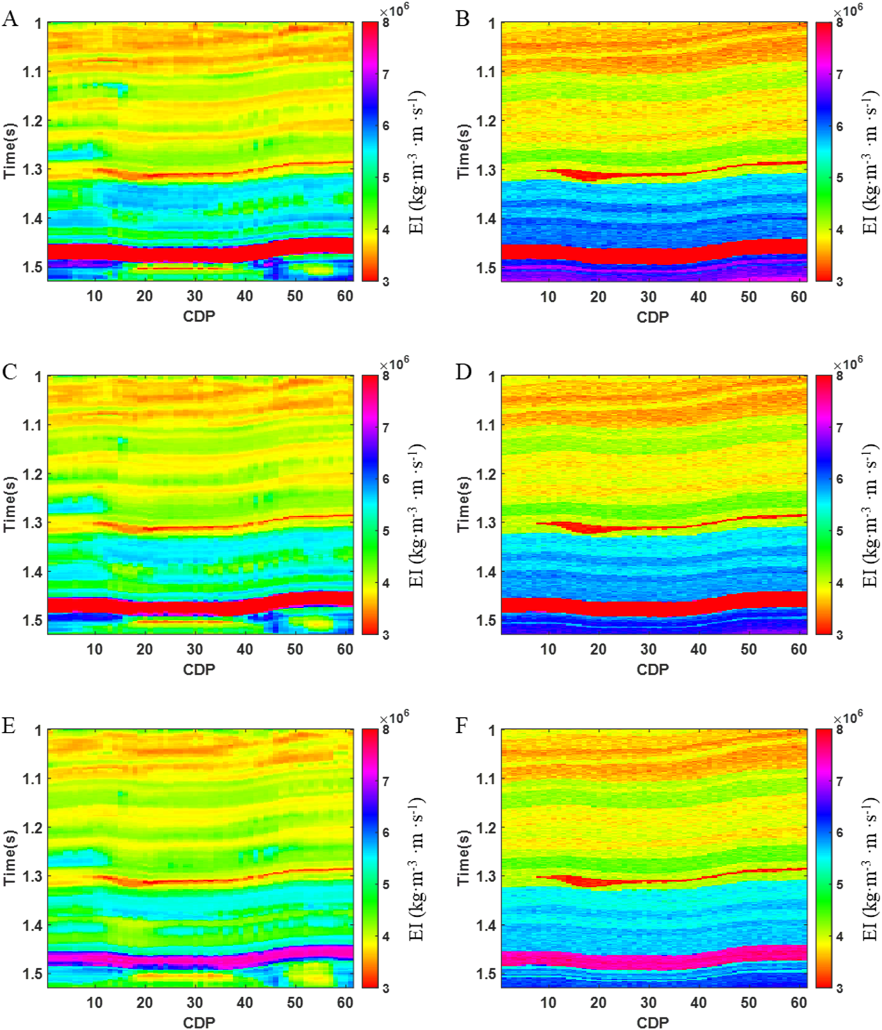
Figure 4. Simulation results of elastic impedance at different angles and elastic impedance inversion results. (A) Near angle elastic impedance simulation result, (B) Near angle elastic impedance inversion result, (C) Middle angle elastic impedance simulation result, (D) Middle angle elastic impedance inversion result, (E) Far angle elastic impedance simulation result, (F) Far angle elastic impedance inversion result.

Figure 5

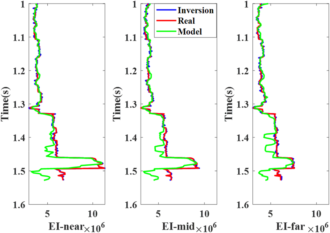
Figure 5. Comparison of single trace inversion results. Blue is the inversion result, red is the real model and green is the simulation result of the model.

To further validate the advantages of this paper’s method, we perform near angle elastic impedance inversion using the Kriging simulation results from Figure 2E, and compare them with the inversion results obtained using the method outlined in this paper (Figure 4B). Figure 6A shows the inversion results based on the Kriging simulation, and Figure 6B presents box plots of the relative errors for both the inversion results from this paper and those based on the Kriging simulation. As shown in the figure, the relative errors of the red solid line (inversion of the method of this paper) are all smaller than those of the blue solid line (inversion based on the Kriging simulation). The mean relative error for the Kriging-based inversion is 0.040, while the mean relative error for the proposed method is 0.015. This quantitative analysis demonstrates that the inversion results from the method in this paper exhibit improved accuracy, which further confirming its effectiveness.

Figure 6

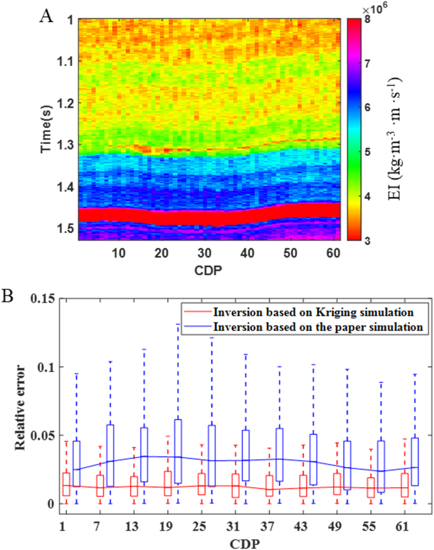
Figure 6. Inversion result based on Kriging simulation and relative error comparison result. (A) Inversion result based on Kriging simulation, (B) Relative error comparison result.

Complex model example

To further validate the applicability of this method to complex models, we use the Stanford model for testing. This model is a fluvial channel system containing deltaic deposits and meandering channels. A section in the Stanford model is taken here for testing. Figure 7A presents the near angle elastic impedance of the real model, in which the oil-bearing reservoir shows a low elastic impedance. Figure 7B displays the near angle seismic data and Figure 7C shows the extracted pseudo-well data. We set the low frequency range to 0–20Hz, the medium frequency range to 20–45Hz, and frequencies greater than 45Hz for the high frequency range. The simulation results for different frequency bands are further established. Figure 8 shows the seismic data for the low (Figure 8A), medium (Figure 8C) and high (Figure 8E) frequency bands, along with the near-angle elastic impedance simulations for each frequency range: low (Figure 8B), medium (Figure 8D) and high (Figure 8F). The simulation results for different frequencies are consistent with the trend of seismic waveform changes at the corresponding frequencies. These results are integrated to obtain the full frequency band simulation, which is then compared with the full-frequency results obtained using the Kriging method. Figure 9A shows the full frequency band elastic impedance simulation results from the Kriging’s method and Figure 9B presents the corresponding results from the proposed method. We calculate the relative errors for the oil-bearing layers based on the two inversion results. For the simulation of oil-bearing reservoir segments, the mean relative error for the Kriging’s method is 0.21, while the mean relative error for the proposed method is 0.13.

Figure 7

Figure 7. Stanford near angle elastic impedance model, synthetic seismic data, and different pseudo-well data. (A) near angle elastic impedance model, (B) near angle synthetic seismic data, (C) pseudo-well.

Figure 8

Figure 8. Stanford near angle seismic data and elastic impedance simulation results at different frequencies. (A) Low frequency near angle seismic data, (B) Low frequency near angle elastic impedance simulation result, (C) Medium frequency near angle seismic data, (D) Medium frequency near angle elastic impedance simulation result, (E) High frequency near angle seismic data, (F) High frequency near angle elastic impedance simulation result.

Figure 9

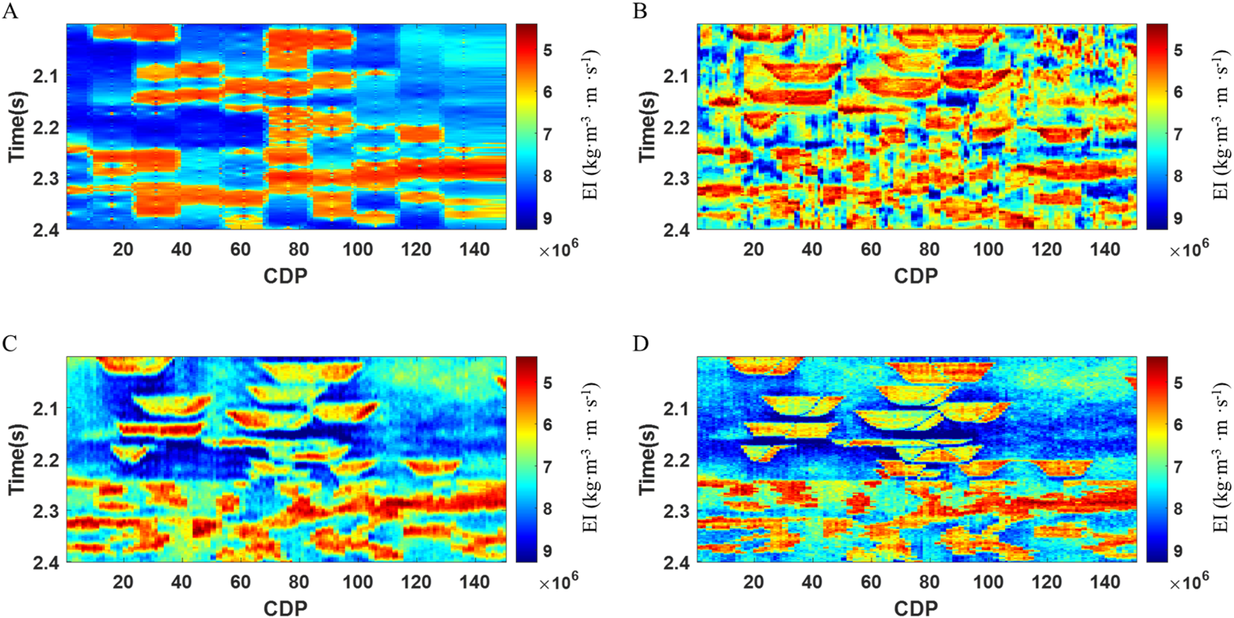
Figure 9. Simulation results and inversion results. (A) Kriging simulation results for Stanford model, (B) Simulation results of this paper’s method for Stanford model, (C) Inversion result based on Kriging simulation, (D) Inversion result based on the paper’s method.

The inversion is further performed based on the two simulation results, respectively. Thus, the inversion results based on the Kriging method (Figure 9C) and the inversion results based on the proposed method (Figure 9D) are obtained. A comparison of the two inversion results shows that the proposed method more clearly delineates the boundaries and distribution of the reservoir. Additionally, when comparing the mean relative errors between the calculated inversion results and the real model, the relative error of the proposed method (0.055) is smaller than that of the Kriging method (0.083). Therefore, this complex model test further verifies the feasibility and advantages of this method.

Field data applications

We conduct the test using field data from a work area in southern China. Figure 10 displays the near angle (Figure 10A), middle angle (Figure 10B) and far angle stacked seismic data (Figure 10C) of the field data. The method proposed in this paper is evaluated using far angle elastic impedance simulations as an example. For this field data test, we also set the low frequency range as 0–20Hz, the medium frequency range as 20–45Hz, and the frequency greater than 45Hz as the high frequency range. Figure 11 shows the low- (Figure 11A), medium- (Figure 11C), and high-frequency (Figure 11E) seismic data corresponding to the far angle seismic data, as well as the results of the far angle elastic impedance simulations for low- (Figure 11B), medium- (Figure 11D), and high-frequency (Figure 11F). It can be observed that the trends of the far angle elastic impedance simulation results at different frequencies are consistent with the trends of the seismic data at different frequencies. The far angle elastic impedance at low, medium and high frequencies is well simulated. However, the low-frequency seismic data at shallow depths exhibit a low signal-to-noise ratio, leading to less continuity in the elastic impedance simulation results at shallow locations. Therefore, the continuity of the simulation results under waveform indication is also limited by the continuity and signal-to-noise ratio of seismic data. Improving the continuity of the simulation results should be considered as the first step to improve the signal-to-noise ratio and continuity of the seismic data.

Figure 10

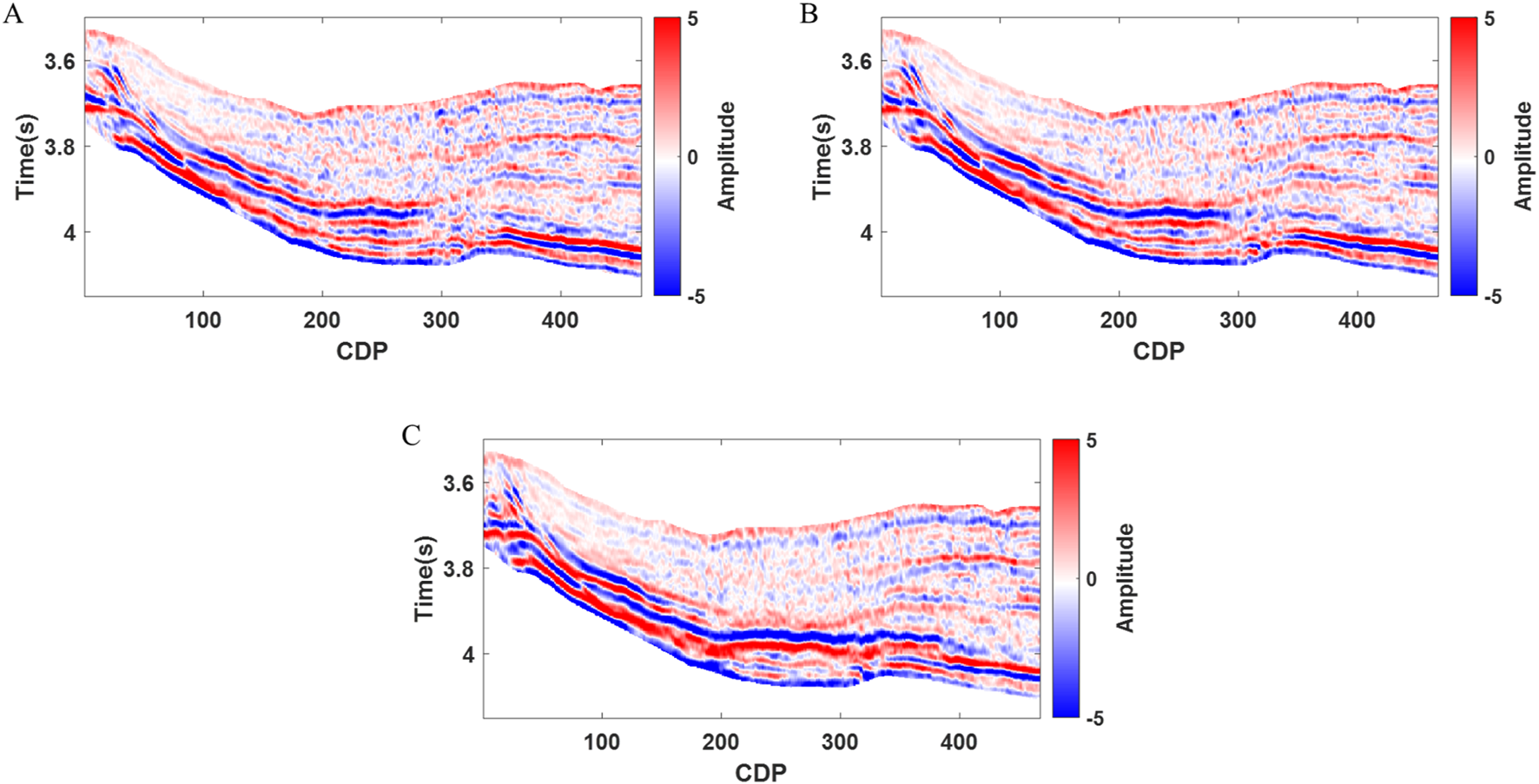
Figure 10. Stacked seismic data at different angles. (A) Near angle stacked seismic data, (B) Middle angle stacked seismic data, (C) Far angle stacked seismic data.

Figure 11

Figure 11. Far angle seismic data and elastic impedance simulation results at different frequencies. (A) Low frequency far angle seismic data, (B) Low frequency far angle elastic impedance simulation results, (C) Medium frequency far angle seismic data, (D) Medium frequency far angle elastic impedance simulation results, (E) High frequency far angle seismic data, (F) High frequency far angle elastic impedance simulation results.

The elastic impedance simulation results at different frequencies are integrated in the frequency domain to obtain the final elastic impedance simulation results at three angles. Figure 12 presents the elastic impedance simulation results for the near angle (Figure 12A), middle angle (Figure 12C) and far angle (Figure 12E), respectively. Among them, the elastic impedance simulation results at different angles are all calculated from the corresponding seismic data at different angles. The final elastic impedance inversion results are obtained by further inversion using seismic data from various angles. Figure 12 also shows the elastic impedance inversion results at near angle (Figure 12B), middle angle (Figure 12D) and far angle (Figure 12F). In these inversion results, the black curve represents the elastic impedance curve from the logging data, and the black elliptical box indicates the location of the gas-bearing reservoir. According to the previous statistical analysis of the logging data, the elastic impedance at the gas-bearing reservoir location shows a low value. From the inversion results, it is evident that the elastic impedance inversion results from three different angles exhibit low values at the gas-bearing reservoir location. And the inversion results match well with the logging curve and exhibit good lateral continuity. Figure 13 displays the well side trace inversion results and logging data histograms at different angles. The histograms reveal that both the well side trace inversion results and the logging curves are consistent with the Gaussian distribution, and the distribution trend and distribution pattern are consistent. At the same time, we also calculate the relative errors between the well data and the inversion results. Among them, the relative error average for the small-angle, medium-angle, and large-angle elastic impedance are 0.020, 0.018 and 0.026, respectively. The relative errors between the three-angle elastic impedance inversion results and the well data are all small. This also indirectly illustrates the accuracy of the inversion results. Therefore, the field data test effectively demonstrates the accuracy and applicability of the proposed method.

Figure 12

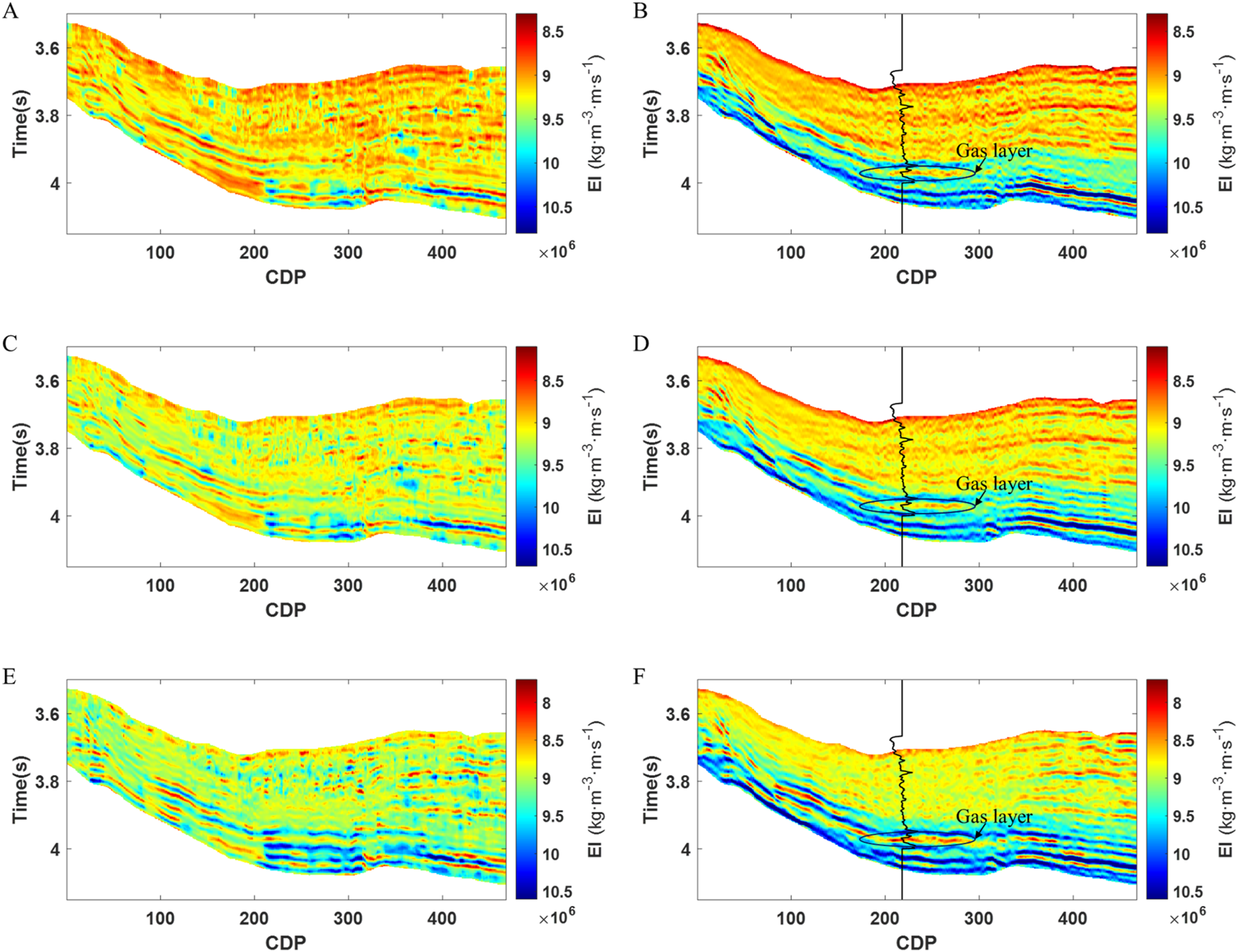
Figure 12. Simulation results of elastic impedance at different angles and elastic impedance inversion results. (A) Near angle elastic impedance simulation result for field data, (B) Near angle elastic impedance inversion result, (C) Middle angle elastic impedance simulation result, (D) Middle angle elastic impedance inversion result, (E) Far angle elastic impedance simulation result, (F) Far angle elastic impedance inversion result.

Figure 13

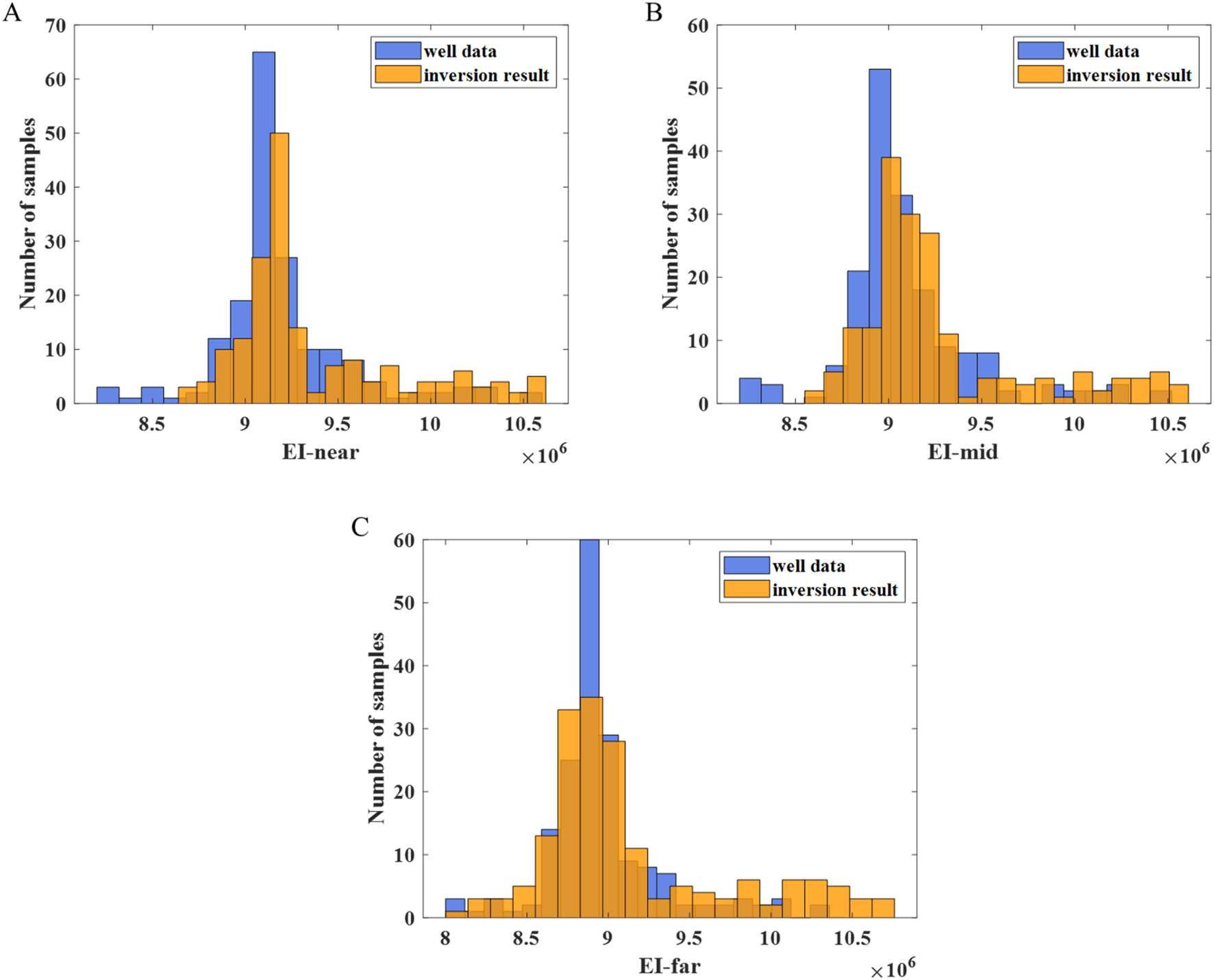
Figure 13. Histograms of well side trace inversion results and logging data at different angles. (A) Near angle elastic impedance histogram, (B) Middle angle elastic impedance histogram, (C) Far angle elastic impedance histogram.

Discussion

The stochastic inversion method based on compressed sensing frequency division waveform indication prior proposed in this paper has contributed to improving the accuracy of low-rank matrix solution, refining the precision of prior information and enhancing the accuracy of inversion results. Compared with the existing methods in the literature, the proposed method effectively mitigates the instability of matrix solving and improves the accuracy of constructing the prior information of oil-bearing layer by introducing the compressed sensing method when dealing with low-rank matrices. In addition, the frequency division modeling method can better simulate reservoir characteristics, especially improve the recognition ability of complex reservoirs. This approach has a significant advantage in addressing the issue of inaccurate prior information, which is common in traditional seismic inversion methods under complex geological conditions.

Most existing waveform indication prior information construction methods depend on simple waveform similarity or traditional kriging interpolation techniques. For example, the waveform indication modeling methods proposed in the work of Zhou et al. (2021) and Yang et al. (2023). However, these methods are unstable during low-rank matrix solving, leading to inaccuracies in the prior information and thus affecting the inversion accuracy. This paper introduces the compressed sensing method to effectively reduce the instability of the calculation when solving the low-rank matrix and improve the accuracy of the prior information. The effectiveness of this method has been validated through both model data testing and field data inversion. Especially in the case of a small number of pseudo wells, the compressed sensing method can still effectively improve the accuracy of constructing prior information of the oil-bearing layer through waveform information, thereby improving the inversion accuracy.

While waveform indicated inversion methods have also been proposed by Shi Y et al. (2024), Chen et al. (2020), and Zhou et al. (2021). However, they did not fully consider the role of different frequency bands of seismic data in the inversion. The proposed method utilizes multi-frequency band modeling technology to establish the prior information of seismic waveform indications. This innovation further improves the accuracy of the inversion results. Especially in the integration of low-frequency and high-frequency information, the proposed method is able to fully exploit the seismic waveform characteristics under different frequency bands. It overcomes the inadaptability of the traditional method to frequency selection, particularly when dealing with strata of different thicknesses. Complex model testing and field data inversion also verified the effectiveness of multi-frequency band modeling technology.

Despite the theoretical and applied advantages of the method in this paper, there are some limitations. Firstly, the compressed sensing method in this paper mainly relies on the Lagrange multiplier optimization method. Although this resolves the instability issue associated with solving low-rank matrices, it introduces high computational complexity, particularly in large-scale field applications. To address this challenge, future work could explore more efficient compressed sensing algorithms or solution strategies based on nonlinear optimization to further improve the computational efficiency and applicability of the algorithms. Secondly, while frequency division modeling can improve the inversion accuracy, it is still a challenge to choose the appropriate frequency band for frequency division modeling. Especially in different geological conditions, the choice of frequency bands may have an impact on the inversion results. Therefore, future studies should further explore how to adaptively select frequency bands according to specific geological characteristics to optimize the inversion effect.

Overall, this paper provides an efficient and accurate seismic inversion method by combining compressed sensing, frequency division waveform indication modeling, and fast simulated annealing algorithm. This method not only breaks through the limitations of traditional methods and improves the mapping accuracy between seismic waveform information and underground reservoir parameters, but also provides strong technical support for field oil and gas exploration.

Conclusion

In this paper, we propose a stochastic inversion method based on compressed sensing frequency division waveform indication prior. This method can fully consider the mapping relationship between the observed seismic data and the parameters to be inverted in different frequency bands through the frequency division method, enabling simulation results that accurately reflect variations in geological bodies of different thicknesses. A more accurate correlation coefficient can be obtained by combining the pseudo-Kriging modeling method with the compressed sensing method. This improves the accuracy of pseudo-Kriging modeling under waveform indication and further improves the simulation accuracy of oil and gas-bearing layers. High quality inversion results are achieved by incorporating more accurate prior information with stochastic inversion methods. Both model and field data demonstrate that the proposed method improves the simulation accuracy of hydrocarbon-bearing reservoirs compared to existing methods, with improvements in both qualitative and quantitative analysis. Furthermore, the combination with stochastic inversion provides higher resolution inversion results. This method accurately characterizes reservoir boundaries and indicates the distribution of underground gas reservoirs. Additionally, the method is not limited to the prediction of elastic impedance, it can also be applied to predict parameters such as P-wave velocity, S-wave velocity and density by combining different reflection coefficient equations to establish prior information and inversion.

Data availability statement

The datasets presented in this article are not readily available because the data analyzed in this study is subject to the following licenses/restrictions: National confidential data. Requests to access the datasets should be directed to eWluZ19fbGluQDE2My5jb20=.

Author contributions

MH: Data curation, Investigation, Methodology, Validation, Writing–original draft, Writing–review and editing. LX: Writing–review and editing. YZ: Writing–review and editing. YH: Writing–review and editing. ZL: Writing–review and editing. YL: Writing–review and editing.

Funding

The author(s) declare that financial support was received for the research, authorship, and/or publication of this article. This paper was funded by the project “Prediction of Paleocene effective reservoir and sweet point description in Enping Yangjiang area of Zhuyi Depression” of CNOOC Shenzhen Branch, Project No. CCL2024SZPS0024.

Acknowledgments

The authors are grateful for the comments provided by the editor and reviewers.

Conflict of interest

Authors MH, LX, YZ, YH, ZL, and YL were employed by CNOOC China Ltd.

Generative AI statement

The author(s) declare that no Generative AI was used in the creation of this manuscript.

Publisher’s note

All claims expressed in this article are solely those of the authors and do not necessarily represent those of their affiliated organizations, or those of the publisher, the editors and the reviewers. Any product that may be evaluated in this article, or claim that may be made by its manufacturer, is not guaranteed or endorsed by the publisher.

References

Basu, A., and Frazer, L. N. (1990). Rapid determination of the critical temperature in simulated annealing inversion. Science 249, 1409–1412. doi:10.1126/science.249.4975.1409

PubMed Abstract | CrossRef Full Text | Google Scholar

Cai, H. P., Ren, H. Y., Wu, Q. P., Peng, L. K., and Wen, C. Y. (2018). “Semi-supervised fast algorithm for seismic waveform classification,” in International geophysical conference 2018 (Beijing: Society of Exploration Geophysicists and Chinese Petroleum Society), 24–27. doi:10.1190/IGC2018-287

CrossRef Full Text | Google Scholar

Chen, S. Y., Cao, S. Y., and Sun, Y. G. (2022). Deblending based on the frequency-structure weighted threshold: the case of the slope-constrained f-k transform. Geophysics 87, V131–V141. doi:10.1190/geo2021-0095.1

CrossRef Full Text | Google Scholar

Chen, Y. H., Bi, J. J., Qiu, X. B., Chen, Y. B., Yang, H., Cao, J. J., et al. (2020). A method of seismic meme inversion and its application. Petroleum Explor. Dev. 47, 1235–1245. doi:10.1016/S1876-3804(20)60132-5

CrossRef Full Text | Google Scholar

Gao, J., Bi, J. J., Zhao, H. S., and Fu, Z. F. (2017). Seismic waveform inversion technology and application of waveform inversion technology and application of thinner reservoir prediction. Prog. Geophys. 32, 142–145. doi:10.6038/pg20170119

CrossRef Full Text | Google Scholar

Gao, X. (2013). Exploration of waveform structure characterization comparison method based on waveform library. Chengdu Univ. Technol.

Google Scholar

Gu, W., Yin, X. Y., Wu, F. R., Li, K., and Zhai, H. J. (2021). Multi-parameter constrained high-resolution inversion method driven by waveform: a case study of Longmaxi Formation shale gas in western Chongqing, Sichuan Basin. Oil Geophys. Prospect. 56, 1311–1321. doi:10.13810/j.cnki.issn.1000-7210.2021.06.014

CrossRef Full Text | Google Scholar

Kirkpatrick, S., Gelatt Jr, C. D., and Vecchi, M. P. (1983). Optimization by simulated annealing. Science 220, 671–680. doi:10.1126/science.220.4598.671

PubMed Abstract | CrossRef Full Text | Google Scholar

Li, K., Yin, X. Y., Zong, Z. Y., and Grana, D. (2022). Estimation of porosity, fluid bulk modulus, and stiff-pore volume fraction using a multitrace Bayesian amplitude-variation-with-offset petrophysics inversion in multiporosity reservoirs. Geophysics 87, M25–M41. doi:10.1190/geo2021-0029.1

CrossRef Full Text | Google Scholar

Lu, Y. J., Cao, J. X., Liu, Z. G., Tian, R. F., and Xiao, X. (2019). Application of waveform classification technology for fluid identification in fractured-vuggy reservoir. Acta Pet. Sin. 40, 182–189. doi:10.7623/syxb201902006

CrossRef Full Text | Google Scholar

Metropolis, N., Rosenbluth, A. W., Rosenbluth, M. N., Teller, A. H., and Teller, E. (1953). Equation of state calculations by fast computing machines. J. Chem. Phys. 21, 1087–1092. doi:10.1063/1.1699114

CrossRef Full Text | Google Scholar

Mosegaard, K., and Vestergaard, P. D. (1991). A simulated annealing approach to seismic model optimization with sparse prior information1. Geophys. Prospect. 39, 599–611. doi:10.1111/j.1365-2478.1991.tb00331.x

CrossRef Full Text | Google Scholar

Shi, S. Z., Gao, W. X., Long, T., Xie, D. S., Li, L., Pei, J. B., et al. (2024). Fine characterization of interbedding sand-mudstone based on waveform indication inversion. J. Geophys. Eng. 21, 396–412. doi:10.1093/jge/gxae010

CrossRef Full Text | Google Scholar

Shi Y, Y., Yu, B., Zhou, H., Cao, Y. M., Wang, W. H., and Wang, N. (2024). FMG_INV, a fast multi-Gaussian inversion method integrating well-log and seismic data. IEEE Trans. Geoscience Remote Sens. 62, 1–12. doi:10.1109/TGRS.2024.3351207

CrossRef Full Text | Google Scholar

Song, C. Y., Qiu, L. P., Chen, Y. Q., and Li, K. H. (2022). Dynamic subwindow matching: a new similarity measure for seismic facies analysis. Geophys. Prospect. 70, 1129–1142. doi:10.1111/1365-2478.13209

CrossRef Full Text | Google Scholar

Srivastava, R. P., and Sen, M. K. (2009). Fractal-based stochastic inversion of poststack seismic data using very fast simulated annealing. J. Geophys. Eng. 6, 412–425. doi:10.1088/1742-2132/6/4/009

CrossRef Full Text | Google Scholar

Wang, B. L., Lin, Y., Zhang, G. Z., Yin, X. Y., and Zhao, C. (2021). Prestack seismic stochastic inversion based on statistical characteristic parameters. Appl. Geophys. 18, 63–74. doi:10.1007/s11770-021-0854-x

CrossRef Full Text | Google Scholar

Xu, Z. Y., Xiong, X. J., Xiao, Y., Zhang, M. Z., Tang, S., and Xiong, G. J. (2022). Reservoir prediction of Sinian Deng 4 member in the intra-platform of Moxi area based on seismic texture attributes clustering method. Prog. Geophys. 37, 1207–1213. doi:10.6038/pg2022FF0248

CrossRef Full Text | Google Scholar

Yang, Y., Gao, A. F., Azizzadenesheli, K., Clayton, R. W., and Ross, Z. E. (2023). Rapid seismic waveform modeling and inversion with neural operators. IEEE Trans. Geoscience Remote Sens. 61, 1–12. doi:10.1109/tgrs.2023.3264210

CrossRef Full Text | Google Scholar

Yu, B., Shi, Y., Zhou, H., Cao, Y. M., Wang, N., and Ji, X. H. (2024). Fast Bayesian linearized inversion with an efficient dimension reduction strategy. IEEE Trans. Geoscience Remote Sens. 62, 1–10. doi:10.1109/TGRS.2024.3360031

CrossRef Full Text | Google Scholar

Zhang, G. Y., Lin, C. Y., and Chen, Y. K. (2020). Convolutional neural networks for microseismic waveform classification and arrival picking. Geophysics 85, WA227–WA240. doi:10.1190/geo2019-0267.1

CrossRef Full Text | Google Scholar

Zhang, S. H., Xu, Y., and Mahdi, A. A. (2016). Characterizing stratigraphic traps using improved waveform classification seismic facies analysis: an example from central Saudi Arabia. First break 34, 12–18. doi:10.3997/1365-2397.34.12.87307

CrossRef Full Text | Google Scholar

Zhao, C., Zhang, G. Z., Cai, H., Zhao, J., Zhang, J. J., and Song, J. J. (2018). Elastic impedance stochastic inversion for P-wave modulus based on FFT-MA simulation and VFQA algorithm. Geophys. Prospect. Petroleum 57, 129–139. doi:10.3969/j.issn.1000-1441.2018.01.017

CrossRef Full Text | Google Scholar

Zhou, D. S. (2015). Quantitative study of seismic waveforms and their application to reservoir prediction. Chengdu Univ. Technol.

Google Scholar

Zhou, S. S., Yin, X. Y., Pei, S., and Yang, Y. M. (2021). Monte Carlo-Markov chain stochastic inversion constrained by seismic waveform. Oil Geophys. Prospect. 56, 543–554.

Google Scholar