A novel seismic inversion method based on multiple attributes and machine learning for hydrocarbon reservoir prediction in Bohai Bay Basin, Eastern China

As the demands for hydrocarbon exploration continue to rise, the identification of thin sand bodies becomes significantly important for subsequent petroleum exploration and development efforts. However, traditional inversion techniques struggle with complex subsurface structures because of the low frequency seismic data. To characterize the architecture of hydrocarbon reservoir precisely, a novel seismic inversion method is applied to improve the resolution of seismic data for a high interpretation accuracy. In this study, we take the X Oilfield in Eastern China as an example, adopted a novel approach combining spectral decomposition with convolutional neural networks (CNNs) within a genetic algorithm (GA) framework for inversion. The CNNs are adept at recognizing and interpreting the spatial configurations in the data, thereby establishing a high correlation between seismic attributes and sand body distributions. GA helps CNNs to get an optimal solution in a fast speed. The results reveal that the model's sand thickness predictions closely match the actual measurements at wells, with a new horizontal well's alignment with the predicted output reaching an accuracy of 85.1%. Compared to traditional seismic inversion methods, our method requires less data. This approach may find a wider application, especially at offshore oilfields with few wells data and low quality seismic data.

1 Introduction

Interpreting seismic data is crucial for mapping out the distribution of reservoir properties and understanding the structure of reservoirs. Techniques in seismic inversion that merge multi-variate stochastic models of rock physics (which connect reservoir characteristics to their elastic properties) with geophysical data are designed to predict various reservoir attributes, such as the layout of sedimentary facies, porosity, and fluid distributions, through mathematical methods (Tounkara et al., 2023; Xie et al., 2023; La Marca et al., 2023). However, the link between seismic information and reservoir features is often ambiguous, hindered by the seismic waves’ limited resolution, the reservoirs’ significant heterogeneity, and the inaccuracies in numerical forward simulations, which may overlook factors like attenuation and noise (Alabbad et al., 2021; Jeong et al., 2017; Lubo-Robles et al., 2023).

Seismic reservoir prediction methods primarily analyze seismic data and comprehensively utilize rock physics, well logging data, and geological information to explore the properties, distribution, and characteristics of underground reservoirs as much as possible, holding a crucial position in the exploration and development of petroleum (De Ruig and Hubbard, 2006; Doyen, 2007). Generally, seismic reservoir prediction methods can be divided into two main categories (Mukerji et al., 2001a; Bosch et al., 2010; Xie et al., 2023): seismic attribute analysis methods and seismic inversion methods (Ulvmoen and Omre, 2010).

Seismic attribute analysis techniques utilize seismic attributes that reflect different geological information to describe the geological characteristics of reservoirs. In the methods of seismic attribute analysis, researchers began to pay attention to the amplitude and polarity of seismic reflections as parameters for identifying oil and gas reservoirs after the seismic attribute extraction technique was introduced (Oliver et al., 2008; Liu et al., 2023). Subsequently, through continuous research and development, seismic attributes have evolved into a series of analysis techniques ranging from classification, extraction, to optimization, such as predicting hydrocarbon potential through the extraction of feature attributes, calculating reservoir parameters from multidimensional attributes; in recent years, with the rapid development of artificial intelligence, the advantage of fitting parameters adaptively through artificial neural network algorithms has been applied to extract rock physics relationships from seismic data, outputting reservoir attributes (Samakinde et al., 2020). However, the core of such methods is to establish a mathematical relationship between attributes and the reservoir, where the results of the reservoir are highly uncertain and lack geological information constraints.

Geophysical inversion methods, fundamentally, are reverse problems that infer causes from results. Broadly speaking, seismic inversion encompasses all seismic interpretation work; from a technical methodological perspective, seismic inversion is based on the kinematic and dynamic parameters of seismic motion. It involves the process of transforming seismic data into reservoir characteristics using the statistical relationship between attributes and known geological information, which is currently a key technology in seismic reservoir prediction. Bosch and others have divided geophysical inversion methods into two types (Mukerji et al., 2001b; Bosch et al., 2010; Xie et al., 2022): sequential or hierarchical methods and Bayesian-based joint simultaneous inversion. Traditional sequential or hierarchical methods transform elastic properties into statistical clustering attributes (probability maps), then used as soft data for geological statistical modeling (Rowbotham et al., 1998; Feng et al., 2019a). Soft data can be considered as an approximate form of data that converts seismic data into probabilities through empirical formulas or fitting formulas to implement regional constraints on the modeling process; in reality, this constraint is based on probability estimates, causing seismic data to lose a lot of seismic information and introducing significant uncertainty into reservoir prediction, which does not reflect the actual underground situation. The joint simultaneous inversion method calculates elastic parameters and reservoir properties at the same time and provides joint uncertainty. The Bayesian framework provides rock physics relationships, combining reservoir properties, elastic parameters, and geological statistical models to establish a prior model that aligns with geological knowledge. By calculating the likelihood function to compare the synthetic data established by forward modeling with the actual observed data, the final posterior distribution obtained conforms to geology, well data, and seismic data (He et al., 2023; Kamenski et al., 2024). Through rock physics relationships, the inversion results more closely match the actual underground conditions, greatly preserving the original seismic data information.

Improving seismic data resolution, integrating geological patterns, and incorporating an optimization algorithm can lead to improved seismic inversion results. Spectral decomposition is employed to generate various dominant frequencies seismic amplitude attributes, thereby enhancing data resolution (Sinha et al., 2005). By using the genetic algorithm (GA), which is based on the biological principles of natural selection, recombination, and mutation of chromosomes (Holland, 1975), this process can be optimized by reducing computation times and producing more precise results. Additionally, Convolutional Neural Networks (CNNs) have proven to be highly effective in extracting features from training sets (Xie et al., 2023). The use of CNNs can lead to more accurate modeling of geological patterns like the distribution of sand bodies, which can be identified from both well interpretations and seismic data.

Our initial approach involves enhancing the quality of seismic data through spectral decomposition. The identification of sand bodies is done by using log interpretation results and attributes from post-stack seismic inversion, which act as quality control factors for training inputs. Finally, a CNN is employed to establish the nonlinear connections between seismic attributes and rock characteristics, with the genetic algorithm further enhancing the training process and improving the model’s accuracy.

2 Methodology

We introduce a new method that combines spectral decomposition with a convolutional neural network-enhanced genetic inversion technique. By spectral decomposition, seismic attributes can be extracted across multiple frequencies, and attributes from higher frequencies provide a higher level of resolution. The improved resolution is particularly beneficial in identifying thin sand bodies, due to the shorter wavelengths and oscillation periods of high-frequency seismic waves, which provide superior spatial detail. The foundation for constructing an improved training dataset for genetic inversion is this attribute, which acts as a data pre-processing step to eliminate unnecessary information.

The core of our method lies in the CNN-based genetic inversion, which is adept at discerning the complex, nonlinear relationships within seismic attributes. The strength of convolutional neural networks is utilized in this approach to recognize and understand patterns, and the genetic algorithm component is employed to refine and optimize the network’s performance. After optimizing, these trained networks are deployed to predict reservoir characteristics.

There are four parts to the method, which begin with spectral decomposition and finish with the use of trained networks for reservoir prediction. The systematic approach of this structured workflow ensures the enhancement of seismic data interpretation and reservoir prediction accuracy.

Initially, we align seismic data with well logs using a time-depth relationship, acknowledging the inherent resolution disparity between the two data types which prevents a straightforward match. To bridge this gap, we engage in a correlation study comparing frequency-decomposed seismic data against sand thickness measurements obtained from log interpretations. The technique of extracting seismic volumes (Marfurt and Kirlin, 2001) at various peak frequencies is used to selectively highlight sand bodies across different temporal thicknesses. The tuning effect is taken into the consideration, a phenomenon that influences how these sand bodies are represented in seismic data due to interference patterns that arise at certain thicknesses (Widess, 1973; Widess, 1983).

In the next step, we utilize well-logging and core data to delineate sand bodies. Core samples offer a high-resolution result that is pivotal for accurate sand identification, facilitating detailed analyses of how these sand bodies correlate with various well log readings like density (DEN), gamma ray (GR), and differential transit time (DT). When core samples are not available, the best alternative, typically gamma ray (GR) logs in well log, is employed for this interpretative work (Wood, 2024). Then, the insights obtained from interpreting these sand bodies are used as benchmarks to validate the integrity and relevance of the training dataset used in convolutional neural networks (CNNs), ensuring that machine learning models are trained on accurate and representative data.

For the last phase, we integrate the processed seismic attributes (FDSVs) as input data into the convolutional neural network (CNN). The CNN is then tasked with identifying and learning the unique patterns within these attributes, guided by pre-provided labels that categorize the data into sand and mud based on previous interpretations. Through the training process, the CNN develops a predictive model, though we have to recognize that this model might initially represent just a local optimum.

To improve the predictive model and potentially overcome the limitations of finding only a local optimal solution, we introduce a genetic algorithm (GA) to find the global optimal solution. The GA adjusts the neural network’s weights and thresholds by multiple iterations, aiming for a more globally optimal solution. This iterative enhancement ensures the network model evolves and improves over time.

Upon achieving an optimized neural network model through this process, we apply it to predict the spatial distribution of sand bodies base on GR value. The output from this optimized model is a continuous volume that distinctly marks the zones identified as GR value, providing a clearer mapping of the reservoirs rock physical properties to wells log.

2.1 Spectral decomposition

In the context of geophysics and seismic data analysis, spectral decomposition is a mathematical method used to transform seismic signals from the time domain into the frequency domain. This is a summary of the principle as follows:

Among the various spectral decomposition techniques available, the Short Time Fourier Transform (STFT) (Goyal and Pabla, 2015) and the Continuous Wavelet Transform (CWT) (Gabry et al., 2024) are two of the most frequently utilized methods. The STFT employs wavelets of a fixed length, which can result in compromised vertical resolution at higher frequencies. The CWT employs wavelets that are relatively short in length and have a fixed number of cycles, which leads to good temporal resolution but can result in poor frequency discrimination when the number of cycles is lower.

The Generalized Spectral Decomposition (GSD) (Li et al., 2019) method offers a hybrid approach that merges the strengths of both STFT and CWT techniques, enabling enhanced control over both vertical and frequency resolution. A set of natural parameters that can be adjusted allows for customized wavelet design between the STFT and CWT approaches to achieve this superior control.

The GSD volume attribute implementation methodology can be summed up in the following steps:

2.1.1 Wavelet design

Customized wavelets can be generated through the use of three key parameters in wavelet computation: frequency, number of cycles, and phase. The original wavelet is then scaled so that it reaches a peak amplitude of one (1.0) in the frequency domain. The custom wavelet is then applied to the input seismic data for decomposition using correlation or filtering using convolution.

2.1.2 Convolution

The initial wavelet is convolved with the input seismic data in the first step. This convolution effectively functions as a band-pass filter, allowing the part of the signal that matches the wavelet to pass through to the output while diminishing the other frequencies.

2.2 CNN-based genetic inversion

The inversion method proposed in this paper is divided into two parts: Convolutional Neural Networks (CNNs) and Genetic Inversion techniques. CNNs are capable of automatically detecting and extracting critical features without manual intervention. This feature extraction is facilitated through multiple convolutional and pooling layers, enabling the network to incrementally learn features from simple to complex. This process significantly enhances the model’s accuracy in prediction and classification tasks.

2.2.1 Convolution neural network

The CNN architecture (Figure 1) comprises an input layer, some convolutional layers, some pooling layers, and a fully connected layer (often referred to as the output layer). More details can be seen as the online tutorials (http://cs231n.github.io/convolutional-networks/). The input layer refines input data (here are seismic volume across various domaint frequencies. The core component of CNN is the convolutional layer, which includes both the convolution kernel and an activation function (in this case, the rectified linear unit (ReLU (Glorot et al., 2011)). The CNN uses convolutional kernels to extract feature maps and employs the activation function to model the nonlinear relationships between the input (training data) and the output (label data).

Figure 1

Figure 1. The structure of CNN.

The input $x$ is transformed into the output $y$ through a network of neurons, which act as computational units following the convolution and pooling layers. The convolution operation is especially advantageous in image classification tasks because of its ability to examine the spatial structures within the input image. For a 2-dimensional CNN, the convolutional layer applies a 3×3 filter ω, and the related equation is given as follows:

$h_{u,v}^k\left(x_{u,v}\right)=f\left({\displaystyle \sum _{i=1}^{N_i}}{\displaystyle \sum _{j=1}^{N_j}}{w}_{i,j}^k{x}_{u+i,v+j}+b\right)(1)$

In Equation 1, $h\left(x\right)$ represents the output of the convolutional layer, $N$ denotes a series of constants, and $w_{i,j}^k$ is an $N_i\times N_j$ filter after the $k$-th training step (where $k$ ($k$ =1, … , $\left.N_k\right)$). Initially, the filter is typically initialized using a Gaussian distribution. The parameter $x_{u,v}$ denote the input with $u,v$ being the pixel coordinates, and $b$ refers to the bias associated with the neuron. Where we use the ReLU activation function $f\left(\ast \right)$ defined as $f\left(x\right)=\max \left(0,x\right)$.

The objective of training a CNN is to determine the optimal weights ($\mathrm{w}$) and biases ($\mathrm{b}$). Typically, reaching the optimal solution demands extensive computational power. Moreover, there is a possibility that the CNN might converge to a local optimum instead of the global one.

2.2.2 Genetic algorithm

Genetic Algorithms (GAs) are a type of heuristic search algorithm that mimics the process of natural selection and genetics. Genetic algorithms have a unique problem-solving approach that has resolved various complex optimization and search challenges across multiple domains. Genetic algorithms are capable of global search, preventing them from stagnating at local optima. This capability allows the algorithm to find superior solutions, especially in scenarios where the solution space is extensive or the optimal solutions are not apparent. Genetic algorithms are adaptable to changing environments and can dynamically adjust their search strategies (Liu et al., 2023). They operate effectively in the absence of a clear analytical solution, making them suitable for complex problems characterized by nonlinearity, multimodality, and discontinuities. Genetic algorithms can also be integrated with other optimization methods to create hybrid algorithms, leveraging the strengths of each to enhance the efficiency and quality of solutions. In this paper, the genetic algorithm can be run by three steps:

(1) Selection: This stage mirrors the concept of natural selection, where individuals exhibiting the least error are chosen. For our study, we derive a fitness function using seismic data and interpretations of sand at well locations, calculated via a least-squares error approach. Individuals, each consisting of a set of weights, are initially selected at random. Those with the best fit form the inaugural generation.

(2) Crossover: In this phase, a collection of weights, termed a chromosome, undergoes a crossover, during which different weight combinations exchange segments. This process facilitates the creation of new optimized combinations, analogous to the random gene swapping seen in natural evolution.

(3) Mutation: To avoid convergence to local minima, mutations are introduced once the error function stabilizes. During this phase, weights are randomly altered, controlled by mutation-specific parameters such as the probability of mutation and the number of mutations involved. Typically, the mutation rate is considerably lower than that of crossover, and it requires significantly less time compared to the neural network’s training duration.

This entire process is repeated until the weights (individuals) are iteratively refined to meet a minimal threshold defined by the loss function. Employing Genetic Algorithms (GA) significantly expedite the neural network training phase and circumvent potential local optima.

3 Application

3.1 Geological background of the X oilfield

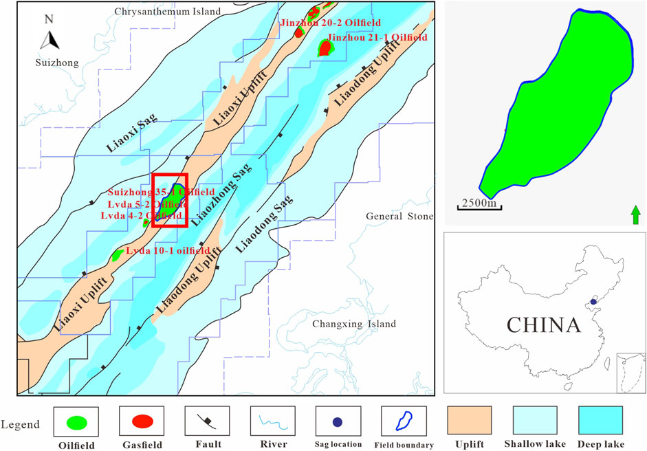
The research area is located in the Liaodong Bay area of eastern China, approximately 50 km northwest of Suizhong City. The average well spacing in the research area is about 150–350 m. The main oil-bearing stratum is the lower part of the Dongying group, featuring a northeastern-oriented faulted anticline. The eastern side transitions to the Liaozhong Depression with a slope, and the western side is bounded by the Liaoxi No.1 fault adjacent to the Liaoxi Depression, constituting an oil and gas reservoir in a buried hill anticline (Figure 2). Vertically, the lower part of the Dongying group is divided into four oil groups: Zero, I, II, and III. This paper mainly considers oil groups I and II, with the reservoir depth ranging from −1,175 to −1,605 m above sea level. The formation thickness is about 350 m, subdivided into 14 sub-layers and 38 individual layers (Zhang et al., 2018). The surface 1, 4-2, and 9 are typical lithological interfaces (the interface is widely developed, with different lithologies above and below, and the physical properties of rocks vary greatly), the seismic response feature is evident to distinguish the time-depth relationship Figure 3.

Figure 2

Figure 2. Location map of the X oilfield in Liaoxi Uplift, China.

Figure 3

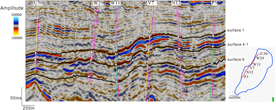
Figure 3. Section of initial seismic data in line P3-U30 (red line in location map). The purple curves represent the GR log and black lines are surfaces (1, 4-1, 9, and 15), the blue line is the boundary of the oil field.

Within the targeted stratigraphic section of the study area, the reservoir lithology is primarily composed of fine sandstone, followed by medium sandstone, with siltstone and coarse sandstone being relatively less common. The main depositional microfacies include lacustrine delta front sand bodies, developing sedimentary microfacies such as mouth bars, distributary channels, and beach sands. The water flow is from west to east of the ancient Suizhong river system (Zhang et al., 2022; Feng et al., 2019b). The sand bodies are continuously distributed and present lobe-shaped, sheet-like, or finger-like patterns. Vertically, they are interbedded with each other, resulting in good connectivity.

The field includes a total of 684 wells, with 227 horizontal wells. Initial seismic data exhibits an effective frequency ranging from 10 Hz to 41 Hz, with a peak at 30 Hz, as indicated in Figure 4. Post-stack seismic data undergoes processing with a 90° phase shift. The sampling for vertical sections is every 2 ms, and the distance between traces is 25 m. Focusing on the third layer, cited studies (Xue et al., 2021) classify it as part of a deltaic depositional system noted for its extensive channel sands. Data from 30 horizontal wells in this third layer serve as an effective dataset for neural network training. The processed seismic data, with its 90° phase shift, reveals that areas displaying lower seismic amplitudes correspond to lower GR values. Conversely, the majority of thinner strata with low GR values demonstrate no significant reactions in the initial seismic attributes.

Figure 4

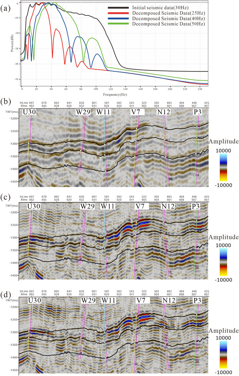
Figure 4. Seismic attributes correlation after frequency decomposition. (A) The frequency spectrum of various seismic volumes; (B) seismic section with a dominant frequency of 25 Hz; (C) seismic section with a domain frequency of 40 Hz; (D) seismic section with a dominant frequency of 50 Hz. All sections come from Figure 3.

3.2 Spectral decomposition

Initial seismic readings indicate a prevalent frequency range between 16 and 30 Hz, which is insufficient for dependable seismic analysis. By employing spectral decomposition, we gather seismic data across various frequencies. This approach enables us to fine-tune the resonance impact by integrating data from different frequencies (Zeng, 2017). For Ricker wavelet, the maximum resolution for vertical thickness determination is determined by the Rayleigh criterion (Ricker, 1953; Kallweit and Wood, 1982), the equation is shown as follows.

$h_{\mathit{max}}=\frac{{\lambda }_d}{4}=\frac{VT}{4}=\frac{V}{4f_d}=\frac{V}{4\left(1.3f_p\right)}(2)$

In this context, $f_p$ stands for the peak frequency (the maximum frequency), $V$ indicates the stratum average velocity, and $f_d$ refers to the dominant frequency. Within the X oilfield, the thickness of the majority of sand bodies in the target formation is below the vertical seismic resolution threshold (for 30 Hz frequency seismic data at 2,200 m/s wave velocity in this region), leading to significant uncertainties in seismic interpretation.

To improve the resolution of seismic data, we proposed a method based on spectral decomposition. In general, matching pursuit decomposition (MPD) is well-regarded for its effectiveness in precisely extracting high-frequency components (Durka et al., 1996; Wang et al., 2016). MPD-based spectral decomposition is the ideal solution because the initial seismic data often lacks enough high-frequency details. In our approach, MPD-based spectral decomposition extracts three frequency-decomposed seismic volumes (FDSVs) with distinct bandwidths: 25 Hz amplitude attribute with a bandwidth of 10–40 Hz, 40 Hz amplitude attribute with a bandwidth of 20–60 Hz, and 50 Hz amplitude attribute with a bandwidth of 20–80 Hz (as illustrated in Figure 4). Equation 2 can help you tune thickness values for the respective FDSVs, with 31.3 m, 19.56 m, and 15.65 m as the desired thickness resolution.

Our analysis reveals that the 25 Hz frequency-decomposed seismic volume (FDSV) shows a stronger correlation with the well log DT (see Figure 5), while the 50 Hz FDSV aligns more closely with the well log SP. This observation confirms that frequency decomposition techniques are effective in extracting critical high-frequency information from initial seismic data. Additionally, the higher-frequency FDSVs display more detailed architectural features and exhibit better alignment with well logs. Thus, these results underscore the potential of frequency decomposition method in improving subsurface interpretation through seismic attribute analysis.

Figure 5

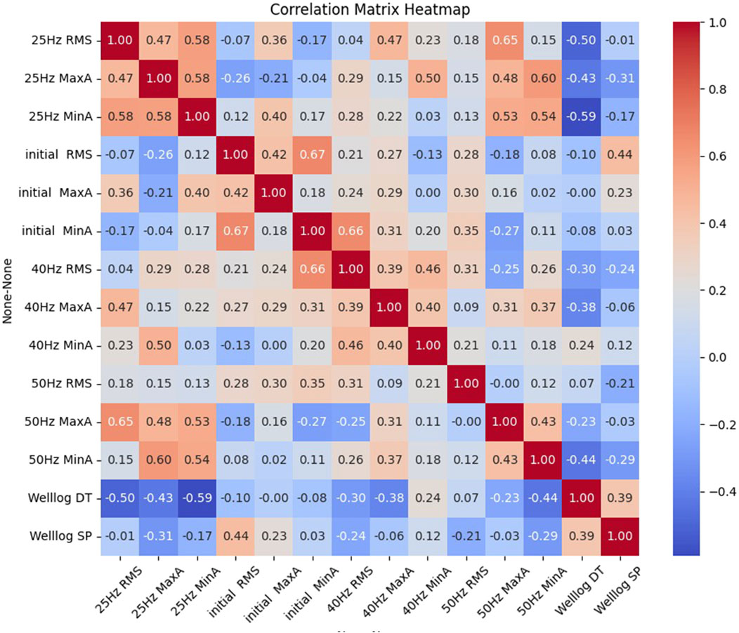
Figure 5. Person correlation coefficient heatmap showing the relationships between the 18 seismic attributes in 4 dominant frequency.

3.3 Facies interpretation

It is necessary to establish labels before the network training phase. Given the uncertainty of underground conditions, obtaining reliable lithological labels may be challenging. The labels for distinguishing sand and mud are defined using core, logging, and seismic data, and GR curves are particularly sensitive to lithological changes. Core is used to identify lithology by correlating logging curves with lithology data to select the most suitable logging curve for distinguishing sand and mud. As shown in Figure 6, the correlation between sand bodies and DT is weak, making traditional seismic impedance inversion ineffective. On the contrary, the GR value shows a strong correlation with sand, making it a valuable parameter for labeling. In this study, GR curves were used as labels for the training set, while FDSV was used as the training dataset.

Figure 6

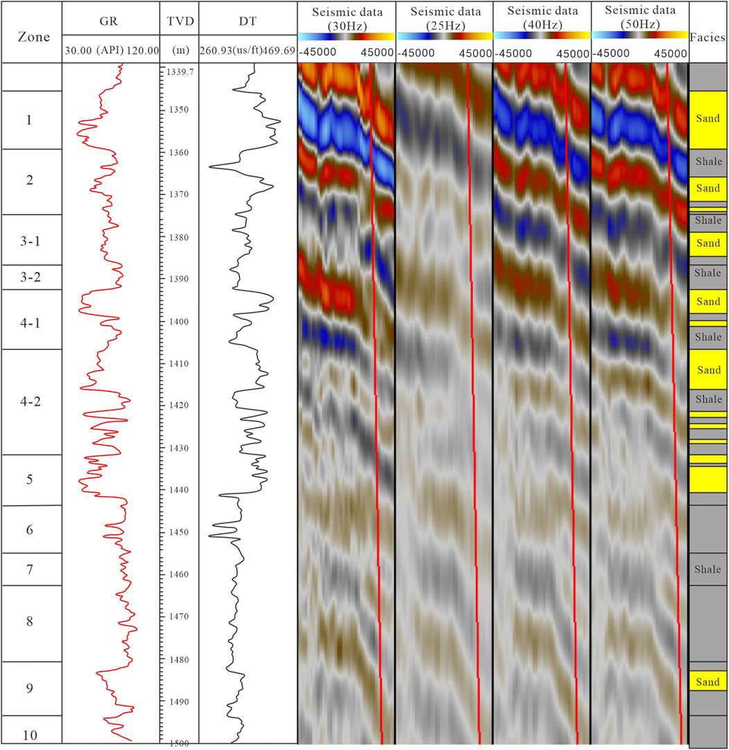
Figure 6. Comparison diagram between different dominant frequency seismic attributes (after 90°conversion) and well logs (the location of well V7 are seen as Figure 3)

3.4 Inversion results

In our test, 300 wells are employed as labels of the learning set, while 20 horizontal wells serve as the test set. The CNN parameters are configured as follows: a median filter with a 3 × 3 × 3 convolution kernel, and the hidden layer is composed of 3 convolutional layers, and the network depth is set to 3 (corresponding to the 3 frequencies FDSVs). The correlated threshold value is established at 0.85, with an iteration decay rate of 0.01. The maximum number of iterations is set to 20,000.

For optimal inversion results and faster convergence in the genetic algorithm, the time window value should closely match the actual seismic wavelet (52 Hz, which is 1.3 times the peak frequency of 40 Hz). Both the in-line and cross-line half ranges are set to 1, while the resample parameter is 3, and the vertical range is 50.

Using the proposed approach, the inversion results exhibit a strong correlation with the original seismic data and reveal more detailed, refined features. Obtaining high-resolution seismic data is essential before interpreting seismic data. We compare a 90°phase conversion and GR genetic inversion result in a same section profile. From a simple vision, the original seismic data can be divided into three matrix sand body, the inversion result can be described as five matrix sand body, and the mud layers are recognized by inversion attributes value. Due to the uncertainty of seismic data, it is not a convincing interpretation by attributes value. We have to prove the inversion attributes can be sensitive to rock features. In general, geologists describe the architecture by geological patterns and well logs, but there is an uncertainty between wells. The interpretation results or facies of well logs are used to verify the inversion attribute, when the attribute value is consistent to the result or facies, the inversion attributes can be used as the indicator of facies or oil/water interpretation.

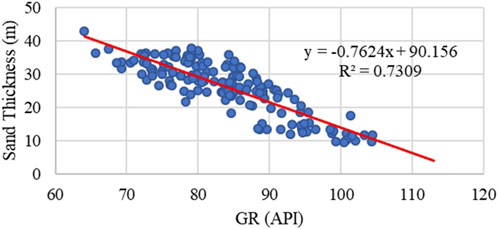
By integrating seismic and well data, the CNN-based genetic inversion method allows for the high-resolution characterization of sand bodies using well data. There are some uncertainties between wells, here a horizontal well is utilized as a test set. Although the thin interbeds are not perfectly characterized, the thick sand bodies in wells are confirmed by the inversion attributes, as shown in Figure 7. Despite this, the method offers a promising improvement in characterization of thin sand bodies, with a resolution that is significantly higher than the initial seismic data. According to the predicted sand thickness, the R² value of 0.7309 compares well to actual measurements (Figure 8). Due to overlap between test and training sets and the inclusion of well-interpreted data in the training data, the high correlation coefficient may be overstated. The correlation of thin sand thickness (for sands less than 10 m thick, which were not part of the training set) demonstrates that the proposed method enhances inversion quality and accurately predicts sand body distribution, which is valuable for gas field development.

Figure 7

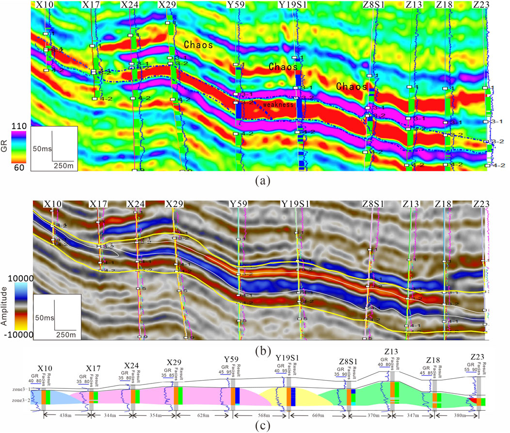
Figure 7. Correlation between inversion result, initial seismic data, and reservoir architecture section. (A) Inversion result, the blue dashed lines represent boundaries of sand bodies in zone 3-2; (B) initial seismic data, yellow lines are the surfaces of zone 3-1 and zone 4-1, white dashed lines are the sand body boundary; (C) architecture section interpreted by production result and well-log, different colors represent different sand bodies.

Figure 8

Figure 8. Correlation relationship analysis between sand thickness (m) and GR value (API) at wells.

The well intersects two channel sand bodies, which differs from the sand interpretation depicted in Figure 9A. Two channel sand bodies are intersected in the well, which is in contrast to the sand interpretation displayed in Figure 9B. The inversion result captures significant geological patterns of the channel, with predicted sand bodies closely aligning with the actual data from the horizontal well (Figure 9C). 32,370 sampling points were provided by the well log curve, which spans 1 km and samples at 0.125-m intervals. The predictions and the points were compared, and it was found that 85.1% (25,419/32,370) of them matched the predictions. The method’s effective reduction of uncertainty in seismic inversion attribute interpretation can be demonstrated through this high accuracy.

Figure 9

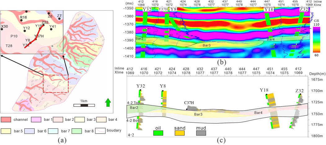
Figure 9. Inversion prediction section and bars interpretation result. (A) Facies map and section location (colors represent bars develop in different times); (B) inversion attribute of C32-E32 section and well logs, blue is GR curve, the green represents sand; (C) sand bodies interpretation section and wells location.

4 Discussion

This study proposes a novel seismic inversion method combined with GA and CNN for predicting the hydrocarbon reservoirs. GA plays an optimal algorithm for fast computing speed, the CNN extract the potential information from seismic attributes and hydrocarbon reservoirs parameters. In marine oil field, few wells and low-quality seismic data make reservoirs prediction difficult. The inversion process can integrate more high-resolution information, which make insufficient data acquire lower uncertainty. When the proposed method is applied to other areas, the training set must be re-built, the FDSVs with different frequency have to be selected after a sand thickness analysis. The label attribute should be the well log with the optimal indicator, for example, the GR curve represent the fraction of mud or sand, the impedance indicates the density and velocity of rocks. After the selection of well log and seismic attributes in training set, the proposed method can be as a tool to run, the best result will be acquired in some minutes.

Compared to the general GA inversion, the CNN is used to extract the nonlinear relation through convolution and activation. Traditional neural networks fail to consider the spatial relation (relation with spatial locations), leading to the seismic inversion result lacking the features of geo-body (Xie et al., 2023a). Then, we use spectral decomposition to generate multiple frequency range seismic attributes, and supply for the reservoir interpretation. Based on the generated attributes and CNN, the high frequency information is added in the low-resolution data from marine oil fields, being an effective way to improve the quality of initial seismic data. Different from conventional seismic inversion, our proposed method calculates a better attribute based on machine learning. It is unnecessary to evaluate the wavelet for seismic impedance, while a precise wavelet is too difficult to acquire. The proposed method overcomes the bias from statistical parameters, and improves the correlation between wells data and seismic data. Genetic algorithm makes the inversion process fast, and CNN digs the potential relation between wells data and seismic data for better prediction of hydrocarbon reservoirs.

In statistical seismic inversion, Bayesian inversion uses statistical modeling methods, such as sequential indicator or multi-point statistical modeling, to generate forward models. The seismic response for each model iteration is calculated and compared with the initial seismic response, and a loss function (see Likelihood Function, Jeong et al., 2017) measures the difference. The model is updated iteratively until the loss function reaches a threshold. Although this approach yields promising results, it often requires numerous iterations and significant computational time. Additionally, acquiring variogram functions and training images can be challenging (Xie et al., 2023b), which may result in models that fail to fully capture natural patterns (Wang et al., 2022a; Wang et al., 2022b). However, advancements in big data and high-performance computing are promising solutions for these challenges.

Recent studies have shown the potential of generative adversarial networks (GANs) in inversion algorithms (Laloy et al., 2018; Xie et al., 2022). GANs can quickly extract complex image features and replicate learned patterns, delivering high-quality inversion results. Despite these advantages, the impact of multi-frequency seismic attributes in GANs is not fully explored. Compared to conventional neural networks, GANs offer significant benefits, and combining them with genetic inversion could further enhance inversion quality and speed.

A key limitation of this method lies in conditioning well data. Since well data is the most accurate source of information, the method prioritizes seismic data and translates a hydrocarbon-sensitive attribute based on well-seismic correction. However, due to the limited resolution of initial marine seismic data, some uncertainty in seismic data remains inevitable. Alternatively, geological modeling can predict hydrocarbon reservoirs by assigning values to spatial grids. This method treats well data as “hard” data while using seismic data as “soft” data to guide interpolation, preserving well data at 100% and using seismic data to fill in inter-well information. Integrating CNN-based inversion with geological modeling could help reduce hydrocarbon reservoir prediction uncertainties. In the future, machine learning algorithms and big data could enable the inclusion of additional hydrocarbon knowledge and insights, improving predictive accuracy and potentially lowering development costs.

Another limitation is the method’s current disregard for faults. Faults significantly influence sand body responses, and their inclusion could support a more continuous interpretation of channel sands. Given the many geological factors that affect seismic response, machine learning applications in this field must incorporate expert geological knowledge for quality control. The next step will involve integrating geological expertise with machine learning algorithms.

When applying this method to other oilfields worldwide, it is essential to consider the specific conditions of the research area. For instance, in mature oilfields with dense well networks (average spacing of 50–300 m), the well data typically have higher resolution than the horizontal resolution of seismic data. Additionally, ample production data reduce uncertainty between wells. In such cases, the inversion results from the proposed method can serve as soft data to decrease hydrocarbon prediction uncertainty, while well data remain critical for reservoir prediction. In offshore oilfields, data scarcity and low-quality seismic data are common due to challenging marine acquisition conditions. These limitations complicate prediction efforts, making the proposed method a promising approach to address low-resolution data issues. Similarly, deep reservoirs face similar challenges, including significant drilling costs and increased seismic noise due to depth, resulting in fewer wells and lower-quality seismic data. The proposed method offers a practical solution to improve reservoir prediction in such scenarios.

5 Conclusion

This study proposes a novel seismic inversion method combined with GA and CNN for predicting the hydrocarbon reservoirs. In this method, the CNN is used to extract the nonlinear relation through convolution and activation. Traditional neural networks fail to consider the spatial relation (relation with spatial locations), leading to the seismic inversion result lacking the features of geobody. The spectral decomposition generates multiple frequency range seismic attributes, and supply for the reservoir interpretation. Based on CNN, the low-resolution data from marine oil fields is added the high frequency information, being an effective way to improve the quality of initial seismic data. The result shows that these sand bodies can be accurately predicted, and their predicted volumes accurately reflect seismic and well data at the specified target level. Also, there is a significant correlation between horizontal well logging and these predictions. Using this method, a significant amount of seismic data and related information can be integrated more effectively. Compared to traditional seismic inversion methods, this approach may find a wider application, especially at offshore oilfields with few wells data and low quality seismic data. In the future, researchers plan to improve deep learning models to recognize geological patterns more accurately and increase processing speed by utilizing high performance computing and parallel computing.

Data availability statement

The original contributions presented in the study are included in the article/supplementary material, further inquiries can be directed to the corresponding author.

Author contributions

ZL: Funding acquisition, Resources, Writing–original draft. JZ: Funding acquisition, Resources, Writing–original draft. BT: Writing–original draft. RZ: Writing–original draft. YF: Data curation, Writing–review and editing. YL: Data curation, Writing–review and editing. LW: Writing–review and editing.

Funding

The author(s) declare that financial support was received for the research, authorship, and/or publication of this article. This research is supported by the National natural science foundation No.42402153 and No.42372137.

Acknowledgments

Parts of this work was supported by the AI tools, include grammar checker software Ginger Software (v 2.3.23) and generative AI Chat GPT4o.

Conflict of interest

Authors ZL, JZ, BT, RZ, YF, and YL were employed by CNOOC China Limited.

The remaining author declares that the research was conducted in the absence of any commercial or financial relationships that could be construed as a potential conflict of interest.

Publisher’s note

All claims expressed in this article are solely those of the authors and do not necessarily represent those of their affiliated organizations, or those of the publisher, the editors and the reviewers. Any product that may be evaluated in this article, or claim that may be made by its manufacturer, is not guaranteed or endorsed by the publisher.

References

Alabbad, A., Dvorkin, J., Altowairqi, Y., and Duan, Z. F. (2021). Rock physics based interpretation of seismically derived elastic volumes. Front. Earth Sci. 8. doi:10.3389/feart.2020.620276

CrossRef Full Text | Google Scholar

Bosch, M., Mukerji, T., and Gonzalez, E. F. (2010). Seismic inversion for reservoir properties combining statistical rock physics and geostatistics: a review. Geophysics 75 (5), 75A165–75A176. doi:10.1190/1.3478209

CrossRef Full Text | Google Scholar

De Ruig, M. J., and Hubbard, S. M. (2006). Seismic facies and reservoir characteristics of a deep-marine channel belt in the Molasse foreland basin, Puchkirchen Formation, Austria. AAPG Bull. 90 (5), 735–752. doi:10.1306/10210505018

CrossRef Full Text | Google Scholar

Doyen, P. M. (2007). Seismic reservoir characterization: an earth modelling perspective. EAGE.

Google Scholar

Durka, P. J., Kelly, E. F., and Blinowska, K. J. (1996). Time-frequency analysis of stimulus-driven EEG activity by matching pursuit. IEEE 3 (1), 1009–1010. doi:10.1109/iembs.1996.652684

CrossRef Full Text | Google Scholar

Feng, W., Yin, Y., Zhang, C., Duan, T., Zhang, W., Hou, G., et al. (2019a). A training image optimal selecting method based on composite correlation coefficient ranking for multiple-point geostatistics. J. Petroleum Sci. Eng. 179, 292–311. doi:10.1016/j.petrol.2019.04.046

CrossRef Full Text | Google Scholar

Feng, W., Zhang, C., Yin, T., Yin, Y., Liu, J., Zhu, R., et al. (2019b). Sedimentary characteristics and internal architecture of a river-dominated delta controlled by autogenic process: implications from a flume tank experiment. Petroleum Sci. 16, 1237–1254. doi:10.1007/s12182-019-00389-x

CrossRef Full Text | Google Scholar

Gabry, M. A., Gharieb, A., Soliman, M. Y., Eltaleb, I., Farouq-Ali, S. M., and Cipolla, C. (2024). Advanced Deep Learning for microseismic events prediction for hydraulic fracture treatment via Continuous Wavelet Transform. Geoenergy Sci. Eng. 239, 212983. doi:10.1016/j.geoen.2024.212983

CrossRef Full Text | Google Scholar

Glorot, X., Bordes, A., and Bengio, Y. (2011). Deep sparse rectifier neural networks. J. Mach. Learn. Res. 15, 315–323.

Google Scholar

Goyal, D., and Pabla, B. S. (2015). Condition based maintenance of machine tools—a review. CIRP J. Manuf. Sci. Technol. 10, 24–35. doi:10.1016/j.cirpj.2015.05.004

CrossRef Full Text | Google Scholar

He, S., Shen, F., Chen, T., Mitri, H., Ren, T., and Song, D. (2023). Study on the seismic damage and dynamic support of roadway surrounding rock based on reconstructive transverse and longitudinal waves. Adv. Geo-Energy Res. 9 (3), 156–171. doi:10.46690/ager.2023.09.04

CrossRef Full Text | Google Scholar

Holland, J. H. (1975). Adaptation in natural and artificial systems. University of Michigan Press.

Google Scholar

Jeong, C., Mukerji, T., and Mariethoz, G. (2017). A fast approximation for seismic inverse modeling: adaptive spatial resampling. Math. Geosci. 49, 845–869. doi:10.1007/s11004-017-9693-y

CrossRef Full Text | Google Scholar

Kallweit, R. S., and Wood, L. C. (1982). The limits of resolution of zero-phase wavelets. Geophysics 47 (7), 1035–1046. doi:10.1190/1.1441367

CrossRef Full Text | Google Scholar

Kamenski, A., Cvetković, M., Kapuralić, J., Močilac, I. K., and Brcković, A. (2024). From traditional extrapolation to neural networks: time-depth relationship innovations in the subsurface characterization of Drava Basin, Pannonian Super Basin. Adv. geo-energy Res. 14 (1), 25–33. doi:10.46690/ager.2024.10.05

CrossRef Full Text | Google Scholar

Laloy, E., Herault, R., Jacques, D., and Linde, N. (2018). Training-image based geostatistical inversion using a spatial generative adversarial neural network. Water Resour. Res. 54 (1), 381–406. doi:10.1002/2017wr022148

CrossRef Full Text | Google Scholar

La Marca, K., Bedle, H., Stright, L., and Marfurt, K. (2023). Sensitivity analysis of seismic attributes parametrization to reduce misinterpretations: applications to deepwater channel complexes. Mar. Petroleum Geol. 153, 106309. doi:10.1016/j.marpetgeo.2023.106309

CrossRef Full Text | Google Scholar

Li, W., Yue, D., Wang, W., Wang, W., Wu, S., Li, J., et al. (2019). Fusing multiple frequency-decomposed seismic attributes with machine learning for thickness prediction and sedimentary facies interpretation in fluvial reservoirs. J. Petroleum Sci. Eng. 177, 1087–1102. doi:10.1016/j.petrol.2019.03.017

CrossRef Full Text | Google Scholar

Liu, Y., Xie, P., Duan, D., Yao, Y., Liu, P., Li, W., et al. (2023). Multiple seismic attributes fusion approach with support vector regression and forward simulation for sand body prediction and sedimentary facies interpretation — a case of the x gas field in xihu sag. Interpretation 11 (1), SA33–SA45. doi:10.1190/int-2021-0213.1

CrossRef Full Text | Google Scholar

Lubo-Robles, D., Bedle, H., Marfurt, K. J., and Pranter, M. J. (2023). Evaluation of principal component analysis for seismic attribute selection and self-organizing maps for seismic facies discrimination in the presence of gas hydrates. Mar. Petroleum Geol. 150, 106097. doi:10.1016/j.marpetgeo.2023.106097

CrossRef Full Text | Google Scholar

Marfurt, K. J., and Kirlin, R. L. (2001). Narrow-band spectral analysis and thin-bed tuning. Geophysics 66 (4), 1274–1283. doi:10.1190/1.1487075

CrossRef Full Text | Google Scholar

Mukerji, T., Avseth, P., Mavko, G., Takahashi, I., and González, E. F. (2001a). Statistical rock physics: combining rock physics, information theory, and geostatistics to reduce uncertainty in seismic reservoir characterization. Lead. Edge 20 (3), 313–319. doi:10.1190/1.1438938

CrossRef Full Text | Google Scholar

Mukerji, T., Jorstad, A., Avseth, P., Mavko, G., and Granli, J. R. (2001b). Mapping lithofacies and pore-fluid probabilities in a North Sea reservoir: seismic inversions and statistical rock physics. Geophysics 66, 988–1001. doi:10.1190/1.1487078

CrossRef Full Text | Google Scholar

Oliver, D. S., Reynolds, A. C., and Liu, N. (2008). Inverse theory for petroleum reservoir characterization and history matching. Cambridge University Press.

Google Scholar

Ricker, N. (1953). Wavelet contraction, wavelet expansion, and the control of seismic resolution. Geophysics 18 (4), 769–792. doi:10.1190/1.1437927

CrossRef Full Text | Google Scholar

Rowbotham, P. S., Lamy, P., Swaby, P. A., and Dubrule, O. (1998). Geostatistical inversion for reservoir characterization. SEG Technical Program Expanded Abstracts, 886–889. doi:10.1190/1.1820631

CrossRef Full Text | Google Scholar

Samakinde, C. A., van Bever Donker, J. M., and Fadipe, O. A. (2020). A combination of genetic inversion and seismic frequency attributes to delineate reservoir targets in offshore northern Orange Basin, South Africa. Open Geosciences 12 (1), 1158–1168. doi:10.1515/geo-2020-0200

CrossRef Full Text | Google Scholar

Sinha, S., Routh, P. S., Anno, P. D., and Castagna, J. P. (2005). Spectral decomposition of seismic data with continuous-wavelet transform. Geophysics 70 (6), P19–P25. doi:10.1190/1.2127113

CrossRef Full Text | Google Scholar

Tounkara, F., Ehsan, M., Nasar Iqbal, M., Al-Ansari, N., Hajana, M. I., Shafi, A., et al. (2023). Analyzing the seismic attributes, structural and petrophysical analyses of the Lower Goru Formation: a case study from Middle Indus Basin Pakistan. Front. Earth Sci. 10. doi:10.3389/feart.2022.1034874

CrossRef Full Text | Google Scholar

Ulvmoen, M., and Omre, H. (2010). Improved resolution in Bayesian lithology/fluid inversion from prestack seismic data and well observations: part 1—methodology. Geophysics 75 (2), R21–R35. doi:10.1190/1.3294570

CrossRef Full Text | Google Scholar

Wang, L., Yin, Y., Zhang, C., Feng, W., Li, G., Chen, Q., et al. (2022a). A MPS-based novel method of reconstructing 3D reservoir models from 2D images using seismic constraints. J. Petroleum Sci. Eng. 209, 109974. doi:10.1016/j.petrol.2021.109974

CrossRef Full Text | Google Scholar

Wang, X., Yu, S., Li, S., and Zhang, N. (2022b). Two parameter optimization methods of multi-point geostatistics. J. Petroleum Sci. and Eng. 208 (B), 109724. doi:10.1016/j.petrol.2021.109724

CrossRef Full Text | Google Scholar

Wang, X., Zhang, B., Li, F., Qi, J., and Bai, B. (2016). Seismic time-frequency decomposition by using a hybrid basis-matching pursuit technique. Interpretation 4 (2), T239–T248. doi:10.1190/int-2015-0208.1

CrossRef Full Text | Google Scholar

Widess, M. B. (1973). How thin is a thin bed? Geophysics 38 (6), 1176–1180. doi:10.1190/1.1440403

CrossRef Full Text | Google Scholar

Widess, M. B. (1983). Addendum to: quantifying resolving power of seismic systems. Geophysics 48 (12), 1687–1690. doi:10.1190/1.1441449

CrossRef Full Text | Google Scholar

Wood, D. A. (2024). Expanding role of borehole image logs in reservoir fracture and heterogeneity characterization: a review. Adv. Geo-Energy Res. 12 (3), 194–204. doi:10.46690/ager.2024.06.04

CrossRef Full Text | Google Scholar

Xie, C., Du, S., Wang, J., Lao, J., and Song, H. (2023). Intelligent modeling with physics-informed machine learning for petroleum engineering problems. Adv. Geo-Energy Res. 8 (2), 71–75. doi:10.46690/ager.2023.05.01

CrossRef Full Text | Google Scholar

Xie, P., Hou, J., Duan, D., Yao, Y., Yang, W., Liu, Y., et al. (2023a). A novel genetic inversion workflow based on spectral decomposition and convolutional neural networks for sand prediction in Xihu Sag of East China Sea. Geoenergy Sci. Eng. 231, 212331. doi:10.1016/j.geoen.2023.212331

CrossRef Full Text | Google Scholar

Xie, P., Hou, J., Wang, Y., Zhang, H., Lv, X., Li, H., et al. (2023b). Application of multi-information fusion modeling of fracture-vuggy reservoir in ordovician reservoir of 12th block in tahe oilfield. J. China Univ. Petroleum Ed. Nat. Sci. 47 (3), 1–14.

Google Scholar

Xie, P., Hou, J., Yin, Y., Chen, Z., Chen, M., and Wang, X. (2022). Seismic inverse modeling method based on generative adversarial networks. J. Petroleum Sci. Eng. 215, 110652. doi:10.1016/j.petrol.2022.110652

CrossRef Full Text | Google Scholar

Xue, Y., Guo, T., Liu, Z., Yu, H., Wang, D., and Zhou, Y. (2021). Accumulation conditions and key technologies for exploration and development of suizhong 36-1 oilfield. Acta Pet. Sin. 42 (11), 1531–1542.

Google Scholar

Zeng, H. (2017). Thickness imaging for high-resolution stratigraphic interpretation by linear combination and color blending of multiple-frequency panels. Interpretation 5 (3), T411–T422. doi:10.1190/int-2017-0034.1

CrossRef Full Text | Google Scholar

Zhang, R., Liu, Z., Jia, X., Wang, G., and Tian, B. (2018). Reservoir plane heterogeneity characterization based on reservoir architecture research. J. Southwest Petroleum Univ. Sci. and Technol. Ed. 40 (5), 15–27.

CrossRef Full Text | Google Scholar

Zhang, R., Liu, Z., Liao, X., Wang, G., and Tian, B. (2022). A study on distribution of remaining oil in the high water-cut stage of delta front sand body. J. Southwest Petroleum Univ. Sci. and Technol. Ed. 44 (2), 1–18.

Google Scholar