Data assimilation by combining ABAQUS with ensemble Kalman filter and its application to geotechnical engineering

Geological parameters of soil exhibit spatial variability. Inverse analysis allows the acquisition of accurate spatial distributions of key geological parameters, which is crucial for structural safety assessment. In this study, an ensemble Kalman filter (EnKF) is employed in the context of data assimilation. Random fields are used as the initial input ensembles for the algorithm. The present study effectively integrates the ensemble Kalman filter with the numerical simulation software ABAQUS, enabling the inversion of parameter fields under various operating conditions. An in-house Python code script is developed to control ABAQUS for finite element computations and to obtain observations at target points. During the stepwise computation process, the algorithm can utilize newly acquired observations to accelerate the convergence of the parameter field to the true field. The effectiveness of the algorithm is validated, and the method is applied to a case study of double-tunnel excavation and a stepwise excavation analysis of a three-layered slope. The impact of the number of ensemble members and the ratio of the horizontal correlation scale to the vertical correlation scale of random fields on the effectiveness of updating the parameter field have also been investigated.

1 Introduction

The stratigraphy of natural environments is formed through prolonged sedimentation, resulting in soil exhibiting heterogeneity. Many scholars regard soil as a complex heterogeneous substance and have demonstrated that soil parameters constitute a spatial stochastic variable (Lumb, 1966), implying that soil parameters possess different values at different locations. Due to the inability to access all material parameters possessed by soil within a given area, rock and soil material parameters are typically treated as stochastic variables. Vanmarcke Erik (1977) presented stochastic models using random fields, achieving more accurate spatial simulations of geological parameters. Building upon the concepts of Vanmarcke’s random field theory, Griffiths and Fenton Gordon (2004) proposed a more rigorous probabilistic analysis method known as the random finite element method (RFEM), which incorporates considerations of spatial correlation length. In RFEM, Monte Carlo methods and random field theory are employed to address the challenge of simulating spatial variability in soil parameters. To tackle the issue of spatial variability in soil parameters, Li X. et al.(2015) focused on the role of conditional random fields. Li et al. (Li et al., 2013; Li Y. J. et al., 2015; Li et al., 2016) concentrated on the domain of three-dimensional slope stability. Furthermore, Li (2017) utilized RFEM to investigate three-dimensional spatial variability in slope stability analysis and conducted performance comparisons with other methods.

Inaccuracies often arise in computational simulations compared to actual engineering scenarios when a crucial geological parameter of the model is crudely defined as a single value. Numerical simulation and monitoring are very important for geohazard and geohazard mitigation (Fang et al., 2023; Fang et al., 2024; Yuan et al., 2024). To address the challenge of obtaining precise soil parameters, the methods of inverse analysis have garnered significant attention in the field of geotechnical engineering. Cividini et al. (1983) employed both the least squares method and Bayesian method to inversely compute Young’s modulus of foundation soil layers based on foundation displacements. Honjo et al. (1994) extended the Bayesian method, while Lee and Kim (1999) applied this approach in tunnel engineering, inversely computing four parameters. Ledesma et al. (1996) provided a brief overview and comparison of four commonly used inverse analysis methods: the least squares method, maximum likelihood method, Bayesian method, and Kalman filtering (KF). Other inverse analysis methods include the Markov Chain Monte Carlo method (MCMC) (Zhang et al., 2010) and the Hamiltonian Monte Carlo method (HMC) (Koch et al., 2020). While inverse analysis methods have shown great potential in geotechnical engineering, they face several challenges, i.e., the bayesian method require numerous forward simulations, which can be computationally expensive for complex geotechnical models. Moreover, traditional methods often struggle to properly account for uncertainties in both measurements and model parameters.

The Kalman filter, particularly the ensemble Kalman filter (Evensen, 1994; Evensen, 2006), and particle filter (Doucet et al., 2000), among other nonlinear methods, have gradually evolved into data assimilation techniques when combined with finite element methods. Among these, EnKF has stood out due to its excellent computational efficiency and has found widespread application. The EnKF has the following advantages over the traditional methods, for example, it provides a probabilistic framework that can handle multiple possible solutions, allowing for sequential updating, which is particularly suited for time-evolving geotechnical problems and it is more computationally efficient. Data assimilation techniques, particularly the Ensemble Kalman Filter (EnKF), have gained significant traction in geotechnical engineering over the past decade. EnKF, originally developed for weather forecasting, has proven to be a powerful tool for integrating observations with numerical models in geotechnical applications. For instance, Chen and Zhang (2006) employed EnKF to update permeability coefficients and pressure heads. Vardon et al. (2016) utilized EnKF to reduce spatial variability in permeability coefficients.

In the context of slope stability, recent studies have shown the potential of data assimilation methods to improve predictions and reduce uncertainties. Liu et al. (2018) proposed a data assimilation framework based on EnKF, utilizing measurements of pore water pressure to improve estimates of hydraulic parameters and consequently predict slope stability. Caballero Perez et al. (2018) enhanced the prediction accuracy of coupled fluid and geomechanical sequential methods at a lower computational cost using EnKF. Li and Liu (2019) combined conditional random fields with EnKF, effectively improving estimates of parameter spatial distributions. Tao et al. (2020) utilized EnKF to investigate key issues in geotechnical and geological domains, such as surface subsidence, and compared simulation results with actual data. Mohsan et al. (2021) combined the EnKF with PLAXIS to investigate the influence of the Mohr-Coulomb model and the Hardening Soil model on the inversion of key parameters in coupled hydro-mechanical slope. Ren et al. (2022) estimated the spatial distribution of the Young’s modulus of an earth-fill dam using EnKF by assimilating arrival times of surface waves.

The use of EnKF for inverse analysis within data assimilation methods requires a forward solver, which in geotechnical engineering is often a custom code script rather than a standardised implementation. In this paper, EnKF is integrated with the numerical simulation software ABAQUS, taking advantage of ABAQUS’ robust problem-solving capabilities. This approach provides a versatile and flexible method for inverse data assimilation analysis, significantly reducing the learning curve associated with this technique.

The main objective of this paper is to achieve parameter updates through EnKF, a data assimilation algorithm. In this process, random fields of critical parameters are generated as the initial input ensemble for filtering. A Python script is employed to control ABAQUS and its subroutines for finite element computations, obtaining observations at each step. This enables the stepwise updating of the parameter field, progressively reducing uncertainties inherent in structural stability analysis. While our work builds upon the foundation laid by Li and Liu (2019), we introduce several innovative aspects. By integrating EnKF with ABAQUS, we extend the applicability of the method to a wider range of complex geotechnical scenarios. Our approach offers enhanced flexibility in problem formulation, improved computational efficiency through optimized scripting, and the ability to handle multi-stage analyses effectively. Furthermore, we provide a comprehensive sensitivity analysis, offering insights into the method’s performance under varying conditions.

The paper is organized into several sections: Section 2 delves into the primary implementation methods of EnKF. A detailed description of the implementation steps and key aspects of the inverse analysis method is provided in Section 3. Section 4 presents a simplified four-step excavation case for comparative analysis and validation of the method’s effectiveness. Section 5 discusses the analysis of a double-tunnel excavation case, focusing on the impact of ensemble size and the ratio of horizontal to vertical fluctuation scales in the random fields on the update results. An analysis of a slope excavation case involving three steps is included in Section 6. The final section is the conclusion of the paper.

2 Ensemble kalman filter

Under normal circumstances, the outcomes of observations come from the observation space. This can be mathematically expressed as follows in Equations 1, 2:

$y=f\left(z\right)(1)$

In which,

$z={\left(z_1,z_2,\dots ,z_n\right)}^T(2)$

in this context, $y\in {\mathbb{R}}^m$ represents the output at measurement points, and $z\in {\mathbb{R}}^n$ denotes a combined vector of model parameters and state variables. Here, $m$ signifies the number of ensembles, while $n$ represents the total count of model parameters and state variables.

Utilizing the algorithm proposed by Evensen (2003), we generate a set of ensembles $X_b$ (Equation 3) of state variable predictions describing the model’s forecast error at time $t_i$. Here, $m$ denotes the number of ensembles:

$X_b=\left\{x_1^b,x_2^b,\dots ,x_m^b\right\}(3)$

In Equation 4, the average value of the set of ensembles of state variables is given by:

$\overline{x^{\mathrm{b}}}=\frac{1}{m}{\displaystyle {\sum }_{i=1}^m}{x}_i^{\mathrm{b}}(4)$

let $x_i^{\prime b}=x_i^b-\overline{x^b}$ denote the difference of the $i$-th ensemble from the mean of ensembles. The matrix representation of these differences can be expressed in Equation 5 as:

$X_b^{\prime }=\left\{x_1^{\prime b},x_2^{\prime b},\dots ,x_m^{\prime b}\right\}(5)$

The covariance matrix of the predicted errors in the state variables can be obtained in Equation 6 as follows:

$B^{\mathrm{f}}=\frac{1}{m-1}{X}^{\prime \mathrm{b}}{\left[X^{\prime \mathrm{b}}\right]}^{\mathrm{T}}(6)$

The calculation formula for error statistics in the Kalman Filter is defined as follows in Equations 7, 8:

$B^{\mathrm{f}}=\overline{\left(X^{\mathrm{b}}-X^{\mathrm{t}}\right){\left[X^{\mathrm{b}}-X^{\mathrm{t}}\right]}^{\mathrm{T}}}(7)$

$B^{\mathrm{a}}=\overline{\left(X^{\mathrm{a}}-X^{\mathrm{t}}\right){\left[X^{\mathrm{a}}-X^{\mathrm{t}}\right]}^{\mathrm{T}}}(8)$

where $B^{\mathrm{a}}$ represents the covariance matrix of analysis errors, $X^{\mathrm{b}}$ represents the analysis state, and $X^{\mathrm{t}}$ denotes the true state. EnKF approximates the ensembles’ mean as the optimal estimate. Centered around the mean, the covariance matrix of the ensembles can be defined as follows in Equations 9, 10:

$B^f\approx \overline{\left(X^{\mathrm{b}}-\overline{X^{\mathrm{b}}}\right){\left(X^{\mathrm{b}}-\overline{X^{\mathrm{b}}}\right)}^{\mathrm{T}}}(9)$

$B^a\approx \overline{\left(X^{\mathrm{a}}-\overline{X^{\mathrm{a}}}\right){\left(X^{\mathrm{a}}-\overline{X^{\mathrm{a}}}\right)}^{\mathrm{T}}}(10)$

Monte Carlo sampling of random numbers is employed to simulate Gaussian white noise with a mean of 0 and a standard deviation equal to the observation multiplied by a noise scaling factor. In this scenario, the displacement vector of measurement points constitutes a set of observations with added perturbations, where the $i$-th sample can be expressed in Equation 11 as:

$y_i=y+y_i^{\prime }(11)$

where the statistical characteristics of $y_i^{\prime }$ exhibit a mean of 0 and an error covariance of $R$. The inclusion of perturbed observations is crucial for EnKF. If the observations are not treated as random variables, the updated ensembles, while possessing the correct mean, may result in excessively low variance, leading to eventual divergence of the algorithm (Burgers et al., 1998).

In Equation 12 the Kalman gain matrix is given by:

$K=B^{\mathrm{f}}{H}^{\mathrm{T}}{\left(H{B}^{\mathrm{f}}{H}^{\mathrm{T}}+R\right)}^{-1}(12)$

where $H$ is the observation operator. $H$ is composed solely of 0s and 1s, and by adjusting its composition, one can succinctly describe the linear or nonlinear relationship between the model and the data.

The primary computational burden of the Kalman filter lies in the calculation of the covariance matrix. In EnKF process, it is evident that the observation operator $H$ and the state error covariance $B^{\mathrm{f}}$ consistently appear in the updating process. Consequently, the operations involving $H$ and $B^{\mathrm{f}}$ can be approximated to replace the actual covariance matrix operations, resulting in a substantial simplification of the computations.

Finally, update the state variables by:

$x_i^{\mathrm{a}}=x_i^{\mathrm{b}}+K\left(y_i-H{x}_i^{\mathrm{b}}\right)(13)$

In Equation 14 the optimal estimate is obtained by taking the mean of $m$ ensembles of state variables:

$\overline{x^{\mathrm{a}}}=\frac{1}{m}{\displaystyle {\sum }_{i=1}^m}{x}_i^{\mathrm{a}}(14)$

The initial value of the state variable are random fields of key geological parameters, which will be updated through EnKF. Upon completion of all iterations, the ensembles’ mean can be regarded as the optimal estimate.

3 Parameter field inversion method using EnKF with ABAQUS

ABAQUS, recognized as a robust finite element analysis software, possesses the capability to simulate a diverse range of mechanical problems and intricate engineering scenarios. It has found widespread application in numerical simulations and engineering computations. Notably, the functionality of ABAQUS subroutines is highly potent. By leveraging these subroutines and connecting them within the ABAQUS framework, various functionalities can be achieved through the utilization of customized Python or Fortran code script. This study specifically employs ABAQUS and its subroutines to assign distinct material parameters to all nodes in the model and to extract displacement values for selected nodes. The flexibility afforded by subroutines ensures the theoretical problem-solving capacity of ABAQUS, rendering it’s theoretically capablity of addressing a spectrum of problems through corresponding inverse analyses.

Accurately predicting the stability of a structure through existing observations is crucial for structural maintenance and safety assessments. The main objective of this paper is to achieve parameter updates through EnKF, a data assimilation algorithm. In this process, random fields of critical parameters are generated as the initial input ensemble for filtering. Customized Python code script is employed to control ABAQUS and its subroutines for finite element computations, obtaining displacement values of the observation points at each step. This enables the stepwise updating of the parameter field, progressively reducing uncertainties inherent in structural stability analysis.

This study utilizes random fields of key geological parameters as the initial ensembles for EnKF. The displacements or stresses at measurement points in the corresponding finite element model are considered as observations. ABAQUS and its subroutines are employed as the computational tools for the model, ultimately achieving the update and inversion of the parameter field.

The general steps of the parameter field inversion method using EnKF with ABAQUS are as follows:

1. Initialization: Generate initial ensemble members using random fields of key parameters. Obtain key parameters such as mean, variance, and spatial correlation from soil data. Use a local averaging subdivision method to generate unconditional random fields of geological parameters to be inverted.

2. Forward Simulation: For each ensemble member, use ABAQUS to simulate the system response. Map the parameters of the random fields to the Abaqus finite element mesh perform finite element analysis.

3. Observation Simulation: Extract simulated observations from ABAQUS output corresponding to measurement locations.

4. EnKF Update: Apply the EnKF update equation to adjust parameter fields based on the difference between simulated and actual observations. The EnKF update equation is given by Equation 13.

5. Use the updated parameter fields for the next round of finite element calculations. Repeat for a specified number of iterations. Upon completion of all iterations, consider the ensembles’ mean as the optimal estimate of the parameter field to be inverted.

The integration with ABAQUS is achieved through custom Python scripts that control the ABAQUS simulations, extract relevant outputs, and feed them into the EnKF algorithm. This approach allows for seamless coupling between the finite element simulations and the data assimilation process. The detailed flowchart of the parameter field inversion method achieved by coupling EnKF with ABAQUS is illustrated in Figure 1.

Figure 1

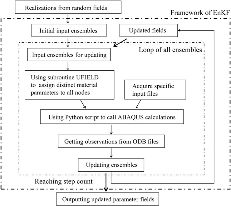
Figure 1. Flowchart of the parameter field inversion method achieved by coupling EnKF with ABAQUS.

In the section on stochastic finite element analysis, an in-house Python code script is employed to map the input parameter field onto the mesh nodes of the computational model. The size of the input parameter field is $N_m\times N_{cell}$, where $N_m$ is the number of ensembles, and $N_{cell}=nxe\times nye$ represents the cell scale of random fields. Initially, the input parameter fields are random fields, serving as the initial ensembles for which the subsequent fields are progressively updated by EnKF. For each ensemble, a parameter field of size $N_{cell}$ is used as the input for finite element calculations. In ABAQUS, a user subroutine called UFIELD is adopted. This ensures that each node in the finite element model can access its corresponding parameter in the mapped parameter field. Subsequently, customized Python code script is utilized to submit computations and obtain displacement values (or stress values at observed Gauss points) corresponding to the measurement points. A snippet of the code is provided in Supplementary Appendix SA.

4 Simplified excavation case for validation

To validate the proposed Abaqus Enkf framework in geotechnical engineering applications, a simplified excavation is considered in this section. Li and Liu (2019) investigated the influence of unconditional and conditional random fields on the inversion of parameter fields. They conducted a computational case study involving the inversion of Young’s modulus for a simplified four-step excavation, as shown in Figure 2. Measurement points were strategically placed within the model, which can obtain observations after each excavation step. These observations were then utilized to update the parameter field. The updated parameter fields were subsequently employed in the next excavation step.

Figure 2

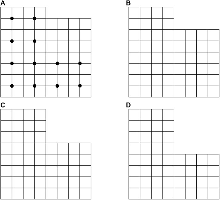
Figure 2. Four-step excavation case: first layer excavation (A) second layer excavation (B) third layer excavation (C) and fourth layer excavation (D) (dots indicate 12 displacement measurement locations).

In this paper, the feasibility of the parameter field inversion method using EnKF with ABAQUS was validated by a reference case study. Li and Liu (2019) used the Enkf with an in-house Fortran finite element code for this case study. The excavation problem assumed in this case had a dimension of $4\mathrm{m}\times 4\mathrm{m}$. The domain is divided into eight-node quadrilateral elements, each with a grid size of $0.5\mathrm{m}\times 0.5\mathrm{m}$. The boundary conditions are fixed base and rollers on left and right sides. The model applied the Mohr-Coulomb failure criterion with $c_u=9\text{kPa}$, $\phi =30°$, $\psi =0.1°$, soil density $\gamma =20\text{kN}/{\mathrm{m}}^3$, and a Poisson’s ratio of 0.49. The inverted parameter field was Young’s modulus field with a mean ${\mu }_E=1.0\times {10}^8\text{Pa}$, coefficient of variation $V_E=0.2$, and isotropic fluctuation scale $\theta =1\mathrm{m}$. The model underwent excavations in four steps, with each excavation depth being $0.5\mathrm{m}$, resulting in a total excavation depth of $2\mathrm{m}$. Simultaneously, parameters such as the number and distribution of measurement points, values of observation noise, etc., were consistent with Li and Liu’s setup (Li and Liu, 2019). For the selection of the reference field, it aligned with Li and Liu’s approach.

When generating unconditional random fields as the initial ensembles, an additional reference field was generated specifically for the current parameter field inversion. To facilitate a better comparison of the two methods in parameter field inversion, both methods utilized the same reference field.

The results of the inversion of Young’s modulus field after the first three excavation steps using Fortran code and the parameter field inversion method using EnKF with ABAQUS are illustrated in Figures 3, 4, respectively. In the plots, cells closer to red indicate higher values, while those closer to blue indicate lower values. For better numerical comparison, the maximum and minimum values in the legend of the plots for each step of both methods are kept identical. Additionally, root mean square error (RMSE) is introduced to better evaluate the results of the parameter field inversion:

$RMSE=\sqrt{\frac{1}{N}{\displaystyle {\sum }_{i=1}^N}{\left(S^t-S^a\right)}^2}(15)$

here, $N$ represents the number of parameters in the parameter field, which, in this case study, is 64. $S^t$ denotes the true parameter field values, and $S^a$ represents the updated parameter field values. The RMSE values for the corresponding parameter fields after three updates using both methods are shown in Figure 5.

Figure 3

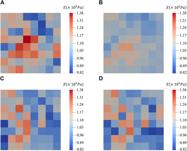
Figure 3. Young’s modulus field using Fortran of: reference field (A) first layer excavation and update (B) second layer excavation and update (C) and third layer excavation and update (D).

Figure 4

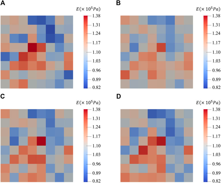
Figure 4. Young’s modulus field using ABAQUS of: reference field (A) first layer excavation and update (B) second layer excavation and update (C) and third layer excavation and update (D).

Figure 5

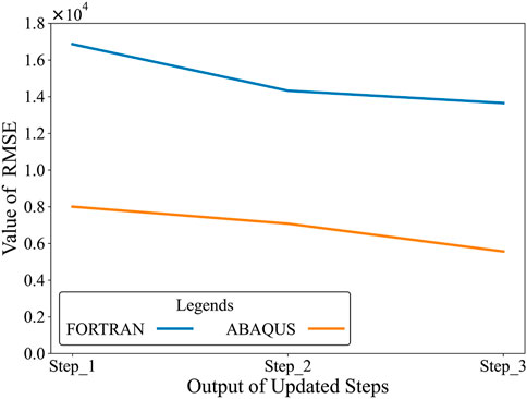
Figure 5. RMSE for Young’s modulus fields after three updates using Fortran and ABAQUS.

Following the first update, the distribution of larger and smaller values in the parameter field is already essentially consistent with the reference field, reflecting the spatial variability of the parameters. However, there is still a significant numerical deviation. This issue sees substantial improvement after the second update, and by the third update, the parameter field is nearly identical to the reference field. As seen in Figure 5, the RMSE values of the parameter fields obtained by the two methods continue to decrease, indicating that the uncertainty of the parameter field decreases continuously under the updating of the algorithm, and the updated parameter field converges to the reference field continuously.

Thus, through the comparison with the results of the four-step excavation case studied by Li and Liu, the feasibility and effectiveness of the parameter field inversion method using EnKF with ABAQUS has been demonstrated.

5 Parameter field inversion of double-tunnel excavation

In the previous section, the feasibility and effectiveness of the parameter field inversion method using EnKF with ABAQUS was validated using a simplified four-step excavation case. In this section, a more complex and realistic two-dimensional double-tunnel excavation case is introduced. The double-tunnel excavation case is selected to demonstrate the applicability of our method to complex, multi-stage geotechnical problems. This case presents challenges in capturing the spatial variability of soil properties and their evolution during sequential excavations, which are common in urban tunneling projects. By applying our EnKF-ABAQUS integration to this scenario, we aim to show how the method can improve parameter field estimations in realistic engineering contexts.

The schematic diagram of the model is shown in Figure 6, with a length of $80\mathrm{m}$ and a height of $40\mathrm{m}$. Moreover, 15 displacement target points are used in this study (the black dot points in Figure 6). The model involves the sequential excavation of two tunnels from left to right, each with a radius of $3\mathrm{m}$. Adjustments have been made to the grids around the tunnels to reduce computational errors. The boundary conditions for the model are fixed base and rollers on left and right sides. The model adopts the Mohr-Coulomb failure criterion, and detailed material parameters are provided in Table 1.

Figure 6

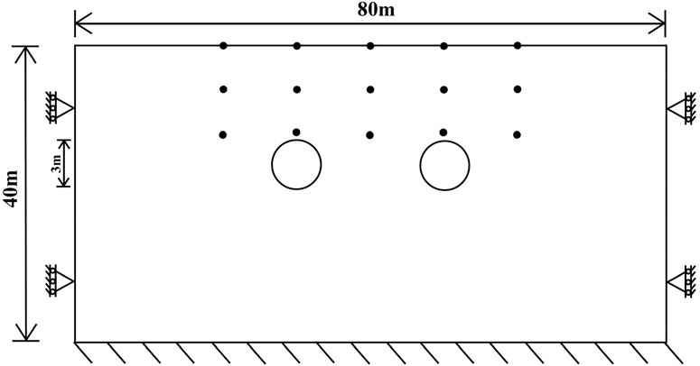
Figure 6. Size and boundary conditions of double-tunnel excavation (dots indicate 15 displacement target points).

Table 1

Table 1. Soil property values of double-tunnel excavation.

According to the parameter sensitivity analysis by Wang et al. (2022), under the Mohr-Coulomb criterion, the sensitivity of displacement values to Young’s modulus is much higher than other parameters. Additionally, since not all elements enter the plastic stage during the simulated excavation process, parameters such as cohesion and friction angle only affect displacement in a few elements. Therefore, in this case, Young’s modulus field is chosen as the parameter field for inversion. To simulate geological stratification and make the inversion results clearer, the reference field is set to have four distinct layers, as shown in Figure 7. Young’s modulus values from top to bottom are: $2.0\times {10}^7\text{Pa}$, $1.7\times {10}^7\text{Pa}$, $2.1\times {10}^7\text{Pa}$ and $2.4\times {10}^7\text{Pa}$. In this Figure, regions closer to red indicate higher Young’s modulus values, while regions closer to blue indicate lower Young’s modulus values.

Figure 7

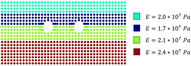
Figure 7. Reference field of Young’s modulus values.

A customized Fortran code was used to generate an unconditional random field of Young’s modulus as the initial ensembles for EnKF. The ensemble size as well as the number of random fields were set to 500. The mean of Young’s modulus was ${\mu }_E=2.0\times {10}^7\text{Pa}$, the coefficient of variation was $V_E=0.15$, the horizontal fluctuation scale ${\theta }_h=16\mathrm{m}$, the vertical fluctuation scale ${\theta }_v=2\mathrm{m}$, resulting in an anisotropy ratio of $aniso={\theta }_h/{\theta }_v=8$. A user subroutine called UFIELD assigned parameter values to all nodes in the model and initiated the computations. Displacement values at measurement points were read from the Odb files, and Gaussian noise with a mean of 0 and a variance of approximately $10\%$ of the surface maximum settlement (1.8 cm in the reference field) was added to the observations.

After the first excavation, the updated parameters were used for the second excavation. The mean of the parameter fields from the 500 ensembles after the two excavations can be considered the best estimate for the parameter field.

The distribution of the parameter field after two excavations is shown in Figure 8. In this Figure, regions closer to red represent higher values, while those closer to blue represent lower values. From Figure 8, it is evident that after the first excavation and update, the distribution of Young’s modulus field already exhibits a clear four-layer pattern, although the boundaries are not well-defined, and there are mixed regions between every two layers. The inversion results for Young’s modulus field in the left edge and right edge regions of the model are not as pronounced. After the second excavation and update, the four-layer pattern, especially in the central region, has clearer boundaries. Young’s modulus field in the left and right regions of the model is now consistent with the reference field, and the distinguishability of Young’s modulus values between the four layers is higher and closer to the corresponding values in the reference field. The trend of RMSE (Equation 15) values for the random fields and the updated fields after two excavations, as shown in Figure 9, also indicates that the inversion of the parameter field has been quite effective after the two-step excavations.

Figure 8

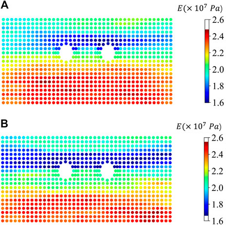
Figure 8. Young’s modulus field of: first tunnel excavation and update (A) second tunnel excavation and update (B).

Figure 9

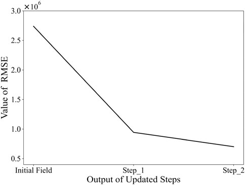
Figure 9. RMSE for Young’s modulus fields of random fields and two updates.

The primary focus is to investigate the influence of the ensemble size and the ratio of the horizontal fluctuation scale to the vertical fluctuation scale $aniso={\theta }_h/{\theta }_v$ on the results of the parameter field inversion.

In the first part of the investigation into the impact of ensemble size on the results of the parameter field inversion, while keeping other parameters constant, the ratio of the horizontal fluctuation scale to the vertical fluctuation scale is set to $aniso={\theta }_h/{\theta }_v=8$. The mean of the observation noise is 0, and the variance is $1\%$ of the maximum displacement value. Figure 10 displays the distribution of the parameter field after one step of update for ensemble sizes of 200, 300, 500, and 1,000, along with the reference field.

Figure 10

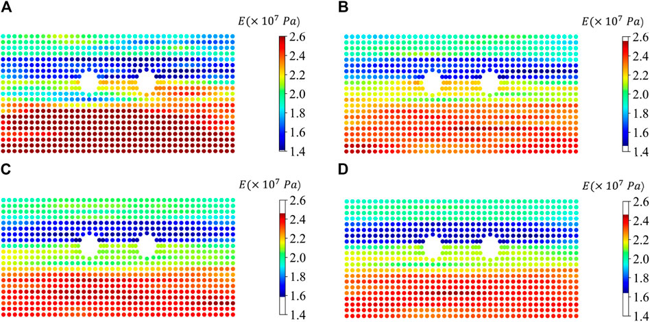
Figure 10. Young’s modulus field of double-tunnel excavation after one update using: 200 ensembles (A) 300 ensembles (B) 500 ensembles (C) 1,000 ensembles (D).

In this Figure, regions closer to red indicate higher Young’s modulus values, while those closer to blue indicate lower values. When the ensemble size is 200, the four-layer stratification in the distribution of the parameter field after one update is almost invisible, with unclear layer boundaries and even mixing between different layers. This outcome is nearly unusable. However, with an increase in the ensemble size, this situation is significantly improved. After one update, the parameter field already exhibits a more distinct four-layer stratigraphic distribution. When the ensemble size is increased to 500, the stratigraphic distribution becomes more apparent, and the contours between each layer are clearer, with no mixing at the layer edges. Increasing the ensemble size to 1,000 does not show a significant improvement compared to an ensemble size of 500, as the results are already fairly close to the reference field. Meanwhile, the RMSE values of the parameter fields for the four ensemble sizes after one update are shown in Figure 11. From this Figure, it can be seen that the curve converges when the ensemble size reaches 500, and further increasing the ensemble size does not lead to a noticeable improvement. It is essential to note that an increase in ensemble size implies a proportional increase in computational cost (i.e. increase the ensemble size from 500 to 1,000 will double the computational cost), as each ensemble’s parameter field undergoes finite element calculation at least once. Considering these factors, an ensemble size of 500 appears to be a reasonable choice for this case.

Figure 11

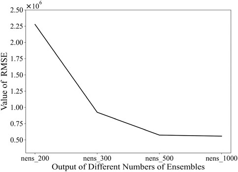
Figure 11. RMSE for Young’s modulus fields using different numbers of ensembles.

Figure 12 presents the probability density distributions of parameter field values for four ensemble sizes after one update, as part of the investigation into the impact of ensemble size on the results of the parameter field inversion. When the ensemble size is 200, the data distribution is extensive, and the four values corresponding to the reference field ($1.7\times {10}^7\text{Pa}$, $2.0\times {10}^7\text{Pa}$, $2.1\times {10}^7\text{Pa}$ and $2.4\times {10}^7\text{Pa}$) are not prominent. This situation persists when the ensemble size increases to 300. However, when the ensemble size reaches 500, three distinct peaks become evident in the data, indicating a more effective reduction of uncertainty in the parameter field updates. With an ensemble size of 1,000, the distribution plot clearly exhibits four peak intervals, ranging from small to large as follows: $1.6725\times {10}^7\sim 1.7\times {10}^7\text{Pa}$, $2.0025\times {10}^7\sim 2.03\times {10}^7\text{Pa}$, $2.1125\times {10}^7\sim 2.14\times {10}^7\text{Pa}$ and $2.36\times {10}^7\sim 2.3875\times {10}^7\text{Pa}$. These values are very close to the four values in the reference field.

Figure 12

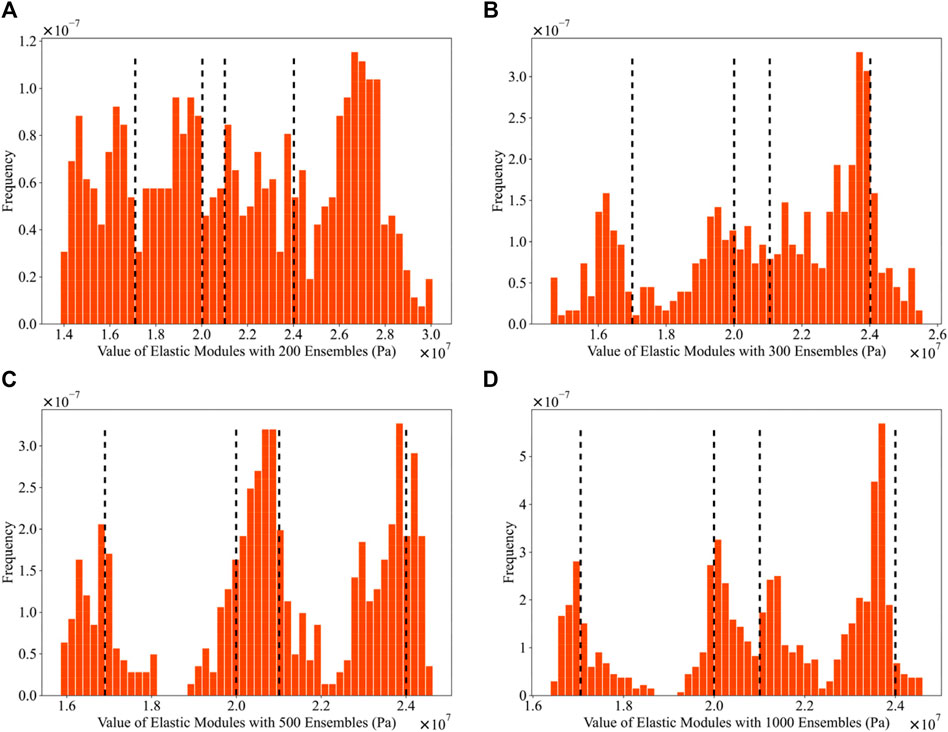
Figure 12. Probability density distributions of Young’s modulus field values after one update using: 200 ensembles (A) 300 ensembles (B) 500 ensembles (C) 1,000 ensembles (D) (The dashed lines in the illustration denote the parameter values of the reference field).

In the second part, the focus is primarily on exploring the impact of the ratio of horizontal to vertical fluctuation scales, denoted as $aniso={\theta }_h/{\theta }_v$, on the results of the parameter field inversion. Other than the aniso values, all other parameters are kept consistent. In this case, the ensemble size is set to $nens=500$, and the mean of the observation noise is 0, with a variance of $1\%$ of the maximum displacement value.

Figure 13 presents the distributions of the reference field and the parameter field after one update for aniso values of 2, 4, 8, 12, 16, and 20. In this Figure, regions closer to red indicate higher values of Young’s modulus, while regions closer to blue indicate lower values. When aniso is set to 2, the parameter field distribution shows almost no discernible four-layer stratification, and the boundaries between layers are relatively unclear, with different layers even exhibiting mixing, making it nearly unusable.

Figure 13

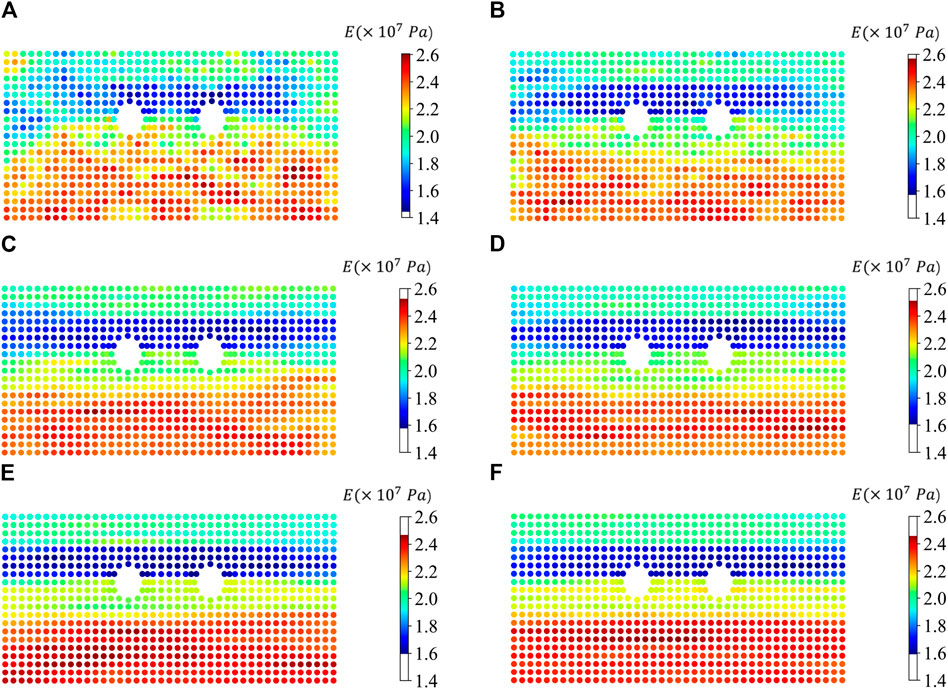
Figure 13. Young’s modulus field of double-tunnel excavation after one update using: $aniso=2$ (A) $aniso=4$ (B) $aniso=8$ (C) $aniso=12$ (D) $aniso=16$ (E) $aniso=20$ (F).

However, when aniso is set to 4 and 8, this situation improves significantly. After one update, the parameter field already exhibits a more apparent stratified distribution, although the contours of the layers are still not very clear, and there are still mixed regions along the edges. When the value of aniso increases to 12, the layer distribution becomes more distinct, with clearer contours between each layer, and the edges of the layers no longer exhibit mixing. When aniso is set to 16 or higher, the parameter field after one update is essentially indistinguishable from the reference field, showing a very clear stratification, and the contours of the layers are highly distinct. Simultaneously, the RMSE values of the parameter field after one update for six values of aniso are shown in Figure 14. From this Figure, it is evident that increasing the value of aniso from 2 to 4 results in a significant improvement in the inversion effectiveness. However, subsequent increases in aniso have a relatively less pronounced impact on the inversion effectiveness. The results depicted in the two Figures can be explained by considering that when the value of aniso is excessively large, the horizontal fluctuation scale approaches the width of the model. As a result, the two-dimensional spatial variability tends to become one-dimensional along the vertical axis, making the inversion much less challenging for one-dimensional data compared to two-dimensional data. In practical geological distributions, layers are unlikely to be so regular and uniformly distributed, rendering excessively large values of aniso meaningless in realistic scenarios.

Figure 14

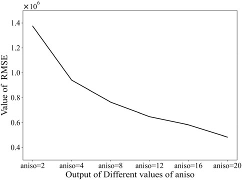
Figure 14. RMSE for Young’s modulus fields using different values of aniso.

Figure 15 presents the probability density distributions of parameter field values after one update for six values of aniso when investigating the influence of the ratio of horizontal to vertical fluctuation scales, denoted as $aniso={\theta }_h/{\theta }_v$. When aniso is set to 2, the data distribution is quite wide, and the four values in the reference field ($1.7\times {10}^7\text{Pa}$, $2.0\times {10}^7\text{Pa}$, $2.1\times {10}^7\text{Pa}$ and $2.4\times {10}^7\text{Pa}$) are not particularly prominent. This situation improves when aniso is set to 4, as three peaks become discernible. When aniso is increased to 8, the data clearly exhibits three peaks, indicating that the parameter field’s update has effectively reduced uncertainty. When aniso is further increased to 16, the distribution graph distinctly presents four peak intervals. The four peaks become more pronounced when aniso is set to 20, with values are $1.64\times {10}^7\sim 1.66\times {10}^7\text{Pa}$, $2.0\times {10}^7\sim 2.02\times {10}^7\text{Pa}$, $2.12\times {10}^7\sim 2.14\times {10}^7\text{Pa}$ and $2.36\times {10}^7\sim 2.38\times {10}^7\text{Pa}$. These values are very close to the values in the reference field.

Figure 15

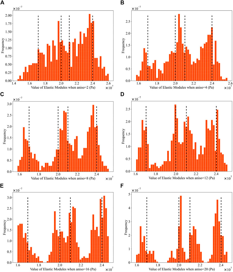
Figure 15. Probability density distributions of Young’s modulus field values after one update using: $aniso=2$ (A) $aniso=4$ (B) $aniso=8$ (C) $aniso=12$ (D) $aniso=16$ (E), $aniso=20$ (F) (The dashed lines in the illustration denote the parameter values of the reference field).

6 Parameter field inversion of slope excavation

In the previous section, we employed a two-dimensional case of a double-tunnel excavation to validate the accuracy of the algorithm and conducted an analysis of relevant parameters. Building upon that foundation, this section will introduce a simplified two-dimensional layered slope with a three-step excavation case for additional validation. The three-layered slope excavation case was chosen to further validate our method in a different geotechnical context and to explore its performance in capturing distinct stratigraphic features. Slope stability analysis is a critical aspect of geotechnical engineering, and accurate estimation of soil parameters in layered slopes is essential for reliable stability assessments. This case study allows us to demonstrate the method’s capability in handling varying spatial correlations and its effectiveness in updating parameter fields across different geological layers.

The schematic diagram of the model is shown in Figure 16, with a length of 240 m, height of 120 m. The three-step excavation is carried out from top to bottom as indicated in the diagram. Excavation sequence is as follows:

1) Initial state: Full slope profile;

2) First excavation: Remove top 20 m from the slope face, part (a) in Figure 16;

3) Second excavation: Remove additional 20 m from the slope face, part (b) in Figure 16

4) Third excavation: Remove final 20 m to achieve the target slope profile, part (3) in Figure 16

Figure 16

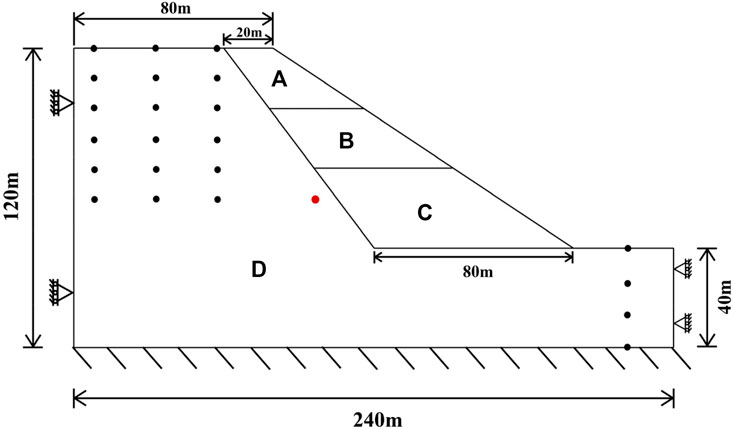
Figure 16. Excavation sequence: first layer excavation (A) second layer excavation (B) third layer excavation (C). (D) Represents the regions involved in the inverse analysis (Black dots indicate displacement measurement locations and the red dot indicates the target point).

Each excavation stage is followed by an EnKF update of the parameter field.

The boundary conditions of the model involve constraining horizontal displacements at both ends, while the bottom is fixed. The model employs the Mohr-Coulomb failure criterion, and detailed material parameters are provided in Table 2.

Table 2

Table 2. Soil property values of slope excavation.

Consistent with the double-tunnel excavation case, a parameter inversion will be conducted for Young’s modulus field. In order to simulate geological stratification and enhance the clarity of the parameter inversion results, a reference field is set with an apparent three-layer stratification, as illustrated in Figure 17. Young’s modulus values are assigned from top to bottom as $5.0\times {10}^9\text{Pa}$、 $6.0\times {10}^9\text{Pa}$ and $8.0\times {10}^9\text{Pa}$. In this Figure, regions with colors closer to red indicate higher values, while regions with colors closer to blue signify lower values.

Figure 17

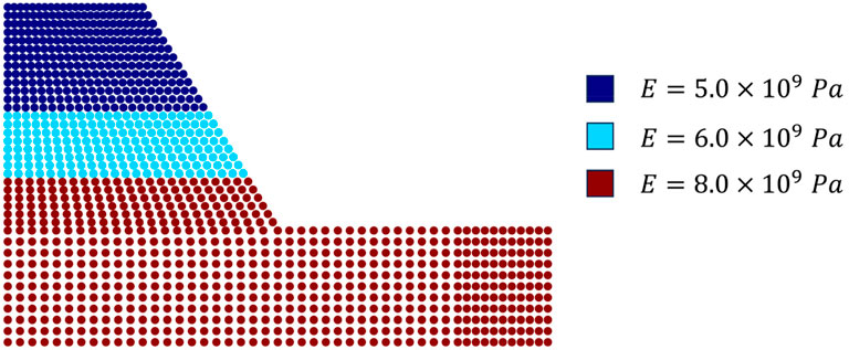
Figure 17. Reference field of Young’s modulus values.

A Fortran code was employed to generate random fields of Young’s modulus for the initial ensembles in EnKF. The ensemble size and the number of random fields remained at 500. The mean of Young’s modulus ${\mu }_E=6.0\times {10}^9\text{Pa}$, the coefficient of variation $V_E=0.2$, the horizontal fluctuation scale ${\theta }_h=24\mathrm{m}$, the vertical fluctuation scale ${\theta }_v=2\mathrm{m}$, resulting in an anisotropy factor of $aniso={\theta }_h/{\theta }_v=12$. Consistent with the double-tunnel excavation case, a user subroutine named UFIELD was used to assign parameter field values to all nodes of the model. Displacement values at observation points were read from the Odb files, with Gaussian noise added to the observations. The mean of the added Gaussian noise was set to 0, and the variance was approximately 10% of the maximum displacement value. After the first excavation and parameter update, the updated parameters were used for the second excavation. Subsequently, the parameters updated after the second excavation were applied to the third excavation. Finally, the mean of the parameter fields from the 500 ensembles was considered as the best estimate for these parameter fields.

The distribution of the parameter field after the three-step excavation update is depicted in Figure 18. In this Figure, regions closer to red indicate higher values, while regions closer to blue signify lower values. From Figure 18, it is obvious that after the first excavation and update, Young’s modulus field distribution has clearly exhibited a three-layer pattern, with distinct edges. Notably, there is no evident lack of inversion effectiveness for Young’s modulus field in the regions at the left and right ends of the model. The results after the first update are superior to the double-tunnel excavation case, primarily due to the increased value of the anisotropy factor (aniso).

Figure 18

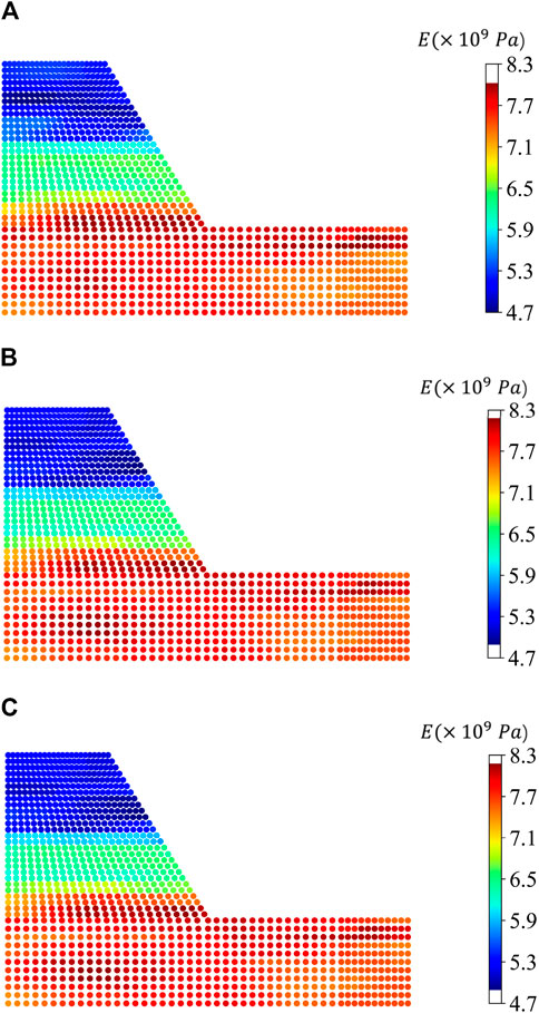
Figure 18. Youngs modulus field of: first excavation and update (A) second excavation and update (B) third excavation and update (C).

In the second and third excavations and updates, the boundary lines of the three-layered region become more distinct. Young’s modulus field at the left and right ends of the model also aligns closely with the reference field, and the discriminability of Young’s modulus values in the three layers is higher, numerically approaching the reference field. The RMSE values for the updated fields of the three-step excavation are shown in Figure 19. After the first excavation and update, the inversion of the parameter field is already quite effective.

Figure 19

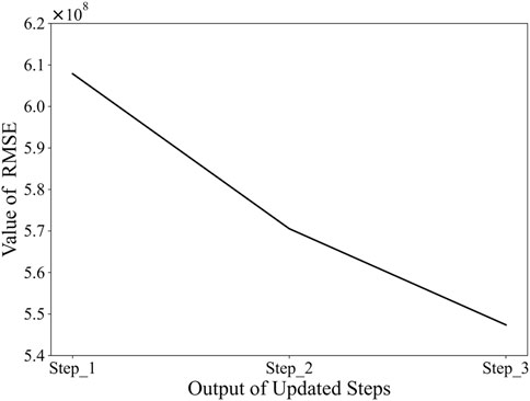
Figure 19. RMSE for Young’s modulus fields of three updates.

As depicted in Figure 16, the red dots therein represent the selected target point. The displacement distribution of this point in both the horizontal and vertical directions under the reference field, as well as within the three successive updating fields, is illustrated in Figure 20. The histograms in the figure depict the distribution of displacements in the horizontal and vertical directions for the target point. The blue curve represents the fitted curve, while the black dashed line signifies the displacements in the horizontal and vertical directions under the reference field for the selected point in the three excavation scenarios. Following each update, the displacement distributions under the parameter fields approximate a normal distribution. Simultaneously, with an increasing number of steps, the mean values of the displacements under the parameter fields converge towards those under the reference field. Additionally, the standard deviation of the displacement distribution progressively decreases. After the three excavation and updating steps, the mean values of the displacements in the horizontal and vertical directions under the updated parameter fields closely resemble those under the reference field, indicating the effectiveness of the parameter field updates.

Figure 20

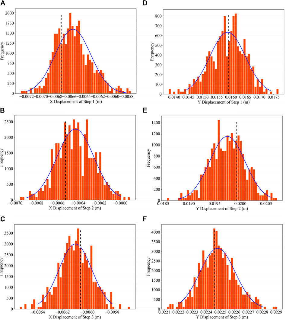
Figure 20. Probability density distributions of target point’s displacement values: in X direction after step 1 (A) in X direction after step 2 (B) in X direction after step 3 (C) in Y direction after step 1 (D) in Y direction after step 2 (E) in Y direction after step 3 (F) (The dashed lines in the illustration denote the target point’s displacement values of three steps under the reference field).

7 Conclusion

This paper presents a parameter field inversion method based on a data assimilation method named EnKF with a finite element analysis tool called ABAQUS. The method employs an ABAQUS subroutine to assign material parameters to nodes, and a customized in-house Python code script is used to control ABAQUS for computations and to read observation points data, which is subsequently utilized for EnKF updates. The method can be applied to various scenarios, including double-tunnel excavation and slope excavation. By using random fields of key parameters as the initial input ensembles for EnKF and utilizing displacement data from observation points, precise inversion of the parameter field can be achieved.

For geological formations characterized by stratified distribution, the ratio of horizontal to vertical fluctuation scales in the random fields, denoted as aniso, significantly influences the results of parameter updates. Similarly, the ensemble size is also a major factor affecting the updating outcomes. In general, a larger ensemble size tends to yield better updating effects. However, a larger ensemble size also implies a greater computational burden. For a specific problem, once the ensemble size reaches a certain value, the improvement in updating results becomes limited.

The results indicate that, owing to higher precision of ABAQUS in finite element computations, this method provides more accurate updates for the parameter field. For multi-step engineering or practical problems, new observations are generated after each step, and these can be utilized for updating the parameter field. Consequently, the parameter field gradually converges to the true values. This characteristic can be beneficial in guiding realistic engineering applications.

The integration with ABAQUS allows for the use of high-performance computing resources to handle more complex and finely discretized models. Future work will focus on optimizing the method for large-scale applications, potentially incorporating techniques such as localization or model reduction to manage computational costs effectively.

Data availability statement

The raw data supporting the conclusions of this article will be made available by the authors, without undue reservation.

Author contributions

DW: Conceptualization, Formal Analysis, Methodology, Writing–original draft. CW: Formal Analysis, Investigation, Methodology, Software, Writing–original draft. XP: Supervision, Validation, Writing–review and editing. HS: Methodology, Resources, Validation, Writing–review and editing. JW: Data curation, Investigation, Validation, Writing–review and editing. ZC: Project administration, Resources, Software, Writing–review and editing.

Funding

The author(s) declare that financial support was received for the research, authorship, and/or publication of this article. The research is supported by the Hunan Provincial Transportation Technology Project (No. 202316).

Conflict of interest

Authors DW, HS, JW, and ZC were employed by Hunan Provincial Water Transportation Construction and Investment Group Co.,Ltd.

The remaining authors declare that the research was conducted in the absence of any commercial or financial relationships that could be construed as a potential conflict of interest.

The reviewer LG declared a shared affiliation with the authors DW, CW to the handling editor at time of review.

Publisher’s note

All claims expressed in this article are solely those of the authors and do not necessarily represent those of their affiliated organizations, or those of the publisher, the editors and the reviewers. Any product that may be evaluated in this article, or claim that may be made by its manufacturer, is not guaranteed or endorsed by the publisher.

Supplementary material

The Supplementary Material for this article can be found online at: https://www.frontiersin.org/articles/10.3389/feart.2024.1456186/full#supplementary-material

References

Burgers, G. J. H., Leeuwen, P. J. v., and Evensen, G. (1998). Analysis scheme in the ensemble kalman filter. Mon. Weather Rev. 126, 1719–1724. doi:10.1175/1520-0493(1998)126<1719:asitek>2.0.co;2

CrossRef Full Text | Google Scholar

Caballero Perez, E. F., Rochinha, F., Borges, M., and Murad, M. (2018). An enhanced ensemble Kalman filter scheme incorporating model error in sequential coupling between flow and geomechanics. Int. J. Numer. Anal. Methods Geomechanics 43, 482–500. doi:10.1002/nag.2872

CrossRef Full Text | Google Scholar

Chen, Y., and Zhang, D. (2006). Data assimilation for transient flow in geologic formations via Ensemble Kalman Filter. Adv. Water Resour. 29, 1107–1122. doi:10.1016/j.advwatres.2005.09.007

CrossRef Full Text | Google Scholar

Cividini, A., Maier, G., and Nappi, A. (1983). Parameter estimation of a static geotechnical model using a Bayes' approach. Int. J. Rock Mech. Min. Sci. & Geomechanics Abstr. 20 (5), 215–226. doi:10.1016/0148-9062(83)90002-5

CrossRef Full Text | Google Scholar

Doucet, A., Godsill, S., and Andrieu, C. (2000). On sequential Monte Carlo sampling methods for Bayesian filtering. Statistics Comput. 10 (3), 197–208. doi:10.1023/A:1008935410038

CrossRef Full Text | Google Scholar

Evensen, G. (1994). Sequential data assimilation with a nonlinear quasi-geostrophic model using Monte Carlo methods to forecast error statistics. J. Geophys. Res. Oceans 99 (C5), 10143–10162. doi:10.1029/94JC00572

CrossRef Full Text | Google Scholar

Evensen, G. (2003). The Ensemble Kalman Filter: theoretical formulation and practical implementation. Ocean. Dyn. 53 (4), 343–367. doi:10.1007/s10236-003-0036-9

CrossRef Full Text | Google Scholar

Evensen, G. (2006). Data assimilation: the ensemble kalman filter. Berlin, Heidelberg: Springer-Verlag.

Google Scholar

Fang, K., Dong, A., Tang, H., An, P., Wang, Q., Jia, S., et al. (2024). Development of an easy-assembly and low-cost multismartphone photogrammetric monitoring system for rock slope hazards. Int. J. Rock Mech. Min. Sci. 174, 105655. doi:10.1016/j.ijrmms.2024.105655

CrossRef Full Text | Google Scholar

Fang, K., Tang, H., Li, C., Su, X., An, P., and Sun, S. (2023). Centrifuge modelling of landslides and landslide hazard mitigation: a review. Geosci. Front. 14 (1), 101493. doi:10.1016/j.gsf.2022.101493

CrossRef Full Text | Google Scholar

Griffiths, D. V., and Fenton Gordon, A. (2004). Probabilistic slope stability analysis by finite elements. J. Geotechnical Geoenvironmental Eng. 130 (5), 507–518. doi:10.1061/(ASCE)1090-0241(2004)130:5(507)

CrossRef Full Text | Google Scholar

Honjo, Y., Wen-Tsung, L., and Guha, S. (1994). Inverse analysis of an embankment on soft clay by extended Bayesian method. Int. J. Numer. Anal. Methods Geomechanics 18 (10), 709–734. doi:10.1002/nag.1610181004

CrossRef Full Text | Google Scholar

Koch, M. C., Fujisawa, K., and Murakami, A. (2020). Adjoint Hamiltonian Monte Carlo algorithm for the estimation of elastic modulus through the inversion of elastic wave propagation data. Int. J. Numer. Methods Eng. 121 (6), 1037–1067. doi:10.1002/nme.6256

CrossRef Full Text | Google Scholar

Ledesma, A., Gens, A., and Alonso, E. E. (1996). Parameter and variance estimation in geotechnical backanalysis using prior information. Int. J. Numer. Anal. Methods Geomechanics 20 (2), 119–141. doi:10.1002/(SICI)1096-9853(199602)20:2<119::AID-NAG810>3.0.CO;2-L

CrossRef Full Text | Google Scholar

Lee, I.-M., and Kim, D.-H. (1999). Parameter estimation using extended Bayesian method in tunnelling. Comput. Geotechnics 24 (2), 109–124. doi:10.1016/S0266-352X(98)00031-7

CrossRef Full Text | Google Scholar

Li, X., Zhang, L., and Li, J. L. (2015a). Using conditioned random field to characterize the variability of geologic profiles. J. Geotechnical Geoenvironmental Eng. 142, 04015096. doi:10.1061/(ASCE)GT.1943-5606.0001428

CrossRef Full Text | Google Scholar

Li, Y. (2017). Reliability of long heterogeneous slopes in 3D: model performance and conditional simulation. PhD thesis. Delft University of Technology.

Google Scholar

Li, Y., Hicks, M. A., and Nuttall, J. (2013) “Probabilistic analysis of a benchmark problem for slope stability in 3D,” in Proceedings of the 3rd international symposium on computational geomechanics (COMGEO III). Krakow, Poland.

Google Scholar

Li, Y., and Liu, K. (2019). Updating soil spatial variability and reducing uncertainty in soil excavations by kriging and ensemble kalman filter. Adv. Civ. Eng. 2019, 1–14. doi:10.1155/2019/8518792

CrossRef Full Text | Google Scholar

Li, Y. J., Hicks, M. A., and Nuttall, J. D. (2015b). Comparative analyses of slope reliability in 3D. Eng. Geol. 196, 12–23. doi:10.1016/j.enggeo.2015.06.012

CrossRef Full Text | Google Scholar

Li, Y. J., Hicks, M. A., and Vardon, P. J. (2016). Uncertainty reduction and sampling efficiency in slope designs using 3D conditional random fields. Comput. Geotechnics 79, 159–172. doi:10.1016/j.compgeo.2016.05.027

CrossRef Full Text | Google Scholar

Liu, K., Vardon, P. J., and Hicks, M. A. (2018). Sequential reduction of slope stability uncertainty based on temporal hydraulic measurements via the ensemble Kalman filter. Comput. Geotechnics 95, 147–161. doi:10.1016/j.compgeo.2017.09.019

CrossRef Full Text | Google Scholar

Lumb, P. (1966). The variability of natural soils. Can. Geotechnical J. 3 (2), 74–97. doi:10.1139/t66-009

CrossRef Full Text | Google Scholar

Mohsan, M., Vardon, P. J., and Vossepoel, F. C. (2021). On the use of different constitutive models in data assimilation for slope stability. Comput. Geotechnics 138, 104332. doi:10.1016/j.compgeo.2021.104332

CrossRef Full Text | Google Scholar

Ren, Y., Nishimura, S., Shibata, T., and Shuku, T. (2022). Data assimilation for surface wave method by ensemble Kalman filter with random field modeling. Int. J. Numer. Anal. Methods Geomechanics 46 (15), 2944–2961. doi:10.1002/nag.3435

CrossRef Full Text | Google Scholar

Tao, Y., Sun, H., and Cai, Y. (2020). Predicting soil settlement with quantified uncertainties by using ensemble Kalman filtering. Eng. Geol. 276, 105753. doi:10.1016/j.enggeo.2020.105753

CrossRef Full Text | Google Scholar

Vanmarcke Erik, H. (1977). Probabilistic modeling of soil profiles. J. Geotechnical Eng. Div. 103 (11), 1227–1246. doi:10.1061/AJGEB6.0000517

CrossRef Full Text | Google Scholar

Vardon, P. J., Liu, K., and Hicks, M. A. (2016). Reduction of slope stability uncertainty based on hydraulic measurement via inverse analysis. Georisk Assess. Manag. Risk Eng. Syst. Geohazards 10 (3), 223–240. doi:10.1080/17499518.2016.1180400

CrossRef Full Text | Google Scholar

Wang, C., Wang, K., Tang, D., Hu, B., and Kelata, Y. (2022). Spatial random fields-based Bayesian method for calibrating geotechnical parameters with ground surface settlements induced by shield tunneling. Acta Geotech. 17 (4), 1503–1519. doi:10.1007/s11440-021-01407-2

CrossRef Full Text | Google Scholar

Yuan, W.-H., Liu, M., Dai, B.-B., Wang, Y., Chan, A., Zhang, W. *, Zheng, X.-C., and Wang, Y. (2024). Stabilizing nodal integration in dynamic smoothed particle finite element method: a simple and efficient algorithm. Comput. Geotechnics 169, 106208. doi:10.1016/j.compgeo.2024.106208

CrossRef Full Text | Google Scholar

Zhang, L. L., Zhang, J., Zhang, L. M., and Tang, W. H. (2010). Back analysis of slope failure with Markov chain Monte Carlo simulation. Comput. Geotechnics 37 (7), 905–912. doi:10.1016/j.compgeo.2010.07.009

CrossRef Full Text | Google Scholar