Uncertainty prediction of conventional gas production in Sichuan Basin under multi factor control

The establishment of a natural gas production model under multi factor control provides support for the formulation of planning schemes and exploration deployment decisions, and is of great significance for the rapid development of natural gas. Especially the growth rate and decline rate of production can be regulated in the planning process to increase natural gas production. The exploration and development of conventional gas in the Sichuan Basin has a long history. Firstly, based on the development of conventional gas production, the influencing factors of production are determined and a production model under multi factor control is established. Then, single factor analysis and sensitivity analysis are conducted, and multi factor analysis is conducted based on Bayesian networks. Finally, combining the multivariate Gaussian mixture model and production sensitivity analysis, a production planning model is established to predict production uncertainty under the influence of multiple factors. The results show that: 1) the production is positively correlated with the five influencing factors, and the degree of influence is in descending order: recovery rate, proven rate, growth rate, decline rate, and recovery degree. After being influenced by multiple factors, the fluctuation range of production increases and the probability of realization decreases. 2) The growth rate controls the amplitude of the growth stage, the exploration rate and recovery rate control the amplitude of the stable production stage, the recovery degree controls the amplitude of the transition from the stable production stage to the decreasing stage, and the decreasing rate controls the amplitude of the decreasing stage. 3)The article innovatively combines multiple research methods to further obtain the probability of achieving production under the influence of multiple factors, providing a reference for the formulation of production planning goals.

1 Introduction

Carbon peaking and carbon neutrality are major national strategies aimed at promoting high-quality economic and social development through the transformation of the energy system, and promoting the transformation of the energy system from fossil energy to renewable energy. Natural gas belongs to low-carbon fossil energy, with a strong development foundation and huge development potential. Moderately leveraging the unique advantages of clean, low-carbon, efficient, and stable natural gas is of great significance for the high-quality development of China’s natural gas industry and the smooth realization of carbon peak and carbon neutrality goals (Song et al., 2023; Nuo et al., 2022; Jian et al., 2018; Jun et al., 2024; Wang et al., 2024; Arun Kumar et al., 2020). In addition, the development of natural gas production is highly uncertain due to various factors such as reserve utilization efficiency, economic factors, geological factors, and development factors (Hongbing and Han, 2023; Haitao et al., 2021; Jianliang and Nu, 2020). Reasonable production target planning is of great significance to the exploration and development of natural gas and can promote the rapid development of natural gas. Therefore, establishing a natural gas production prediction model under multi factor control provides support for the preparation of planning schemes and exploration deployment decisions, and is of great significance for the rapid development of natural gas.

There has been some research on methods and models for predicting natural gas production, and they have been well applied both domestically and internationally. Tongfei and Yanrui, 2022 proposed a new discrete fractional nonlinear grey Bernoulli model with power terms, which has the advantages of most grey prediction models, such as fractional order cumulative operation and time power terms. Then, taking the consumption and production of natural gas in China from 2003 to 2020 as an example, the feasibility and effectiveness of the model were verified. The results indicate that the predictive ability of this model is superior to other models. Chong et al., 2022 established an optimized grey system model with weighted score accumulation, which has good predictive performance. Then, taking the natural gas production of Germany, Italy, and Canada as examples, the feasibility of the model was confirmed through comparison with the competitive model, and the model was used to study China’s natural gas production. The results indicate that this model is very suitable for predicting and analyzing China’s natural gas production. Yingying et al., 2022 established a semi analytical shale gas constant pressure production capacity prediction model and verified it with actual production data. Research has shown that this method has certain theoretical reference value in reducing the risk of production prediction during the production process of shale gas wells and guiding the optimization of development plans. In addition, many scholars have applied algorithms to predict energy sources such as natural gas. Durmuş and Safa, 2022 proposed a new improved Artificial bee colony (M-ABC) method, which adaptively selects the optimal search equation to estimate energy consumption in Turkey more accurately. The results show that the model based on M-ABC algorithm is more successful in estimating energy demand. Durmuş Özdemir (Özdemir et al., 2022) developed a new adaptive artificial bee colony algorithm, which can adaptively select the appropriate search equation to estimate the transportation energy demand more accurately. The results show that the error of this algorithm is lower. (Bilici et al., 2023) compared the performance of four different meta-heuristic algorithms used to estimate gas demand in Turkey. The results show that PSO-Quadratic model is the most successful in predicting observed gas consumption. The research of these scholars has brought some inspiration, and suitable models or algorithms can be used to predict natural gas production.

Although domestic and foreign scholars have optimized production prediction models, these methods all combine models and historical data to predict the development trend of production, without considering factors that affect natural gas production, such as proven rate, recovery rate, decline rate, etc., and are not suitable for environments with multi factor control (Marta et al., 2020; Erick et al., 2022; Palanisamy et al., 2021). Therefore, it is necessary to establish a production target prediction model that considers various influencing factors. Guo et al., 2021 used Monte Carlo probability method to obtain the probability distribution and growth curve of various production risk factors and production of the Carboniferous gas reservoir in eastern Sichuan. In addition, the sensitivity analysis of risk factors was conducted using the fuzzy comprehensive evaluation method, and the natural gas production and realization probability under different risk factors were obtained. Jianzhong et al., 2016 used a gas field in the Ordos Basin as an example to construct an optimal extraction model for natural gas resources. They analyzed the impact of factors such as the extraction scale of the gas field, recovery rate, discount rate, and gas well depletion period on the optimal exploration path of the gas field. Since these studies only consider the impact of a single factor on production, they cannot reflect the coupling effect of multiple factors on production in actual production. Therefore, it is necessary to combine multiple influencing factors and calculate the multivariate probability of production realization. In view of many factors affecting natural gas production, this paper comprehensively considers the change rule and realization probability of production under the influence of different factors, which makes up for the shortcomings of current research. Due to the need to simultaneously consider multiple factors for mixed probability calculation and establish a multi factor prediction model, Bayesian networks and Gaussian mixture models are needed.

Bayesian networks are developed by J Pearl was proposed in the 1980s as a powerful tool for representing, manipulating, and inferring beliefs about the real world. They are used to demonstrate the probability relationships between random variables and serve as models for the joint probability distribution of these variables (Duygu and Derya, 2019; Yaser et al., 2021; Haoran et al., 2022; Jiří et al., 2023; Qi et al., 2018 proposed a fuzzy probability Bayesian network method for dynamic risk assessment. FPBN has been established to analyze and predict the propagation of network security risks, and an approximate dynamic inference algorithm has been proposed for dynamic assessment of ICS network security risks. Yang et al., 2021 proposed a system level fatigue reliability assessment model based on Bayesian networks, treating bridge decks as a parallel system. A fatigue probability reliability model was derived using the main S-N curve. Kyung et al., 2024 realized Bayesian inference of all conditional probabilities within the network at low power and low energy consumption, and achieved a normalized mean squared error of ∼7.5×10⁻⁴ through division feedback logic with variational learning rate to suppress the inherent variation of the memristor. Therefore, Bayesian networks can be used to solve the calculation problem of mixed probabilities of multiple factors.

Gaussian Mixture Model (GMM) is a special type of finite mixture model that assumes that the basic distribution of data is composed of a mixture of multiple Gaussian distributions. GMM has been widely applied in various scientific fields, including computer vision, pattern recognition, and supervised and unsupervised learning (Luca, 2023; Cangqi et al., 2020; Maruf, 2021; Joachim et al., 2024; Zhe et al., 2020 used a Gaussian mixture model to estimate the probability density function of wave height in the context of second-order random wave theory. Two methods were used to construct a Gaussian mixture probability distribution, and three sets of observation data were applied to further validate the accuracy and effectiveness of the Gaussian mixture model; Chunsheng et al., 2020 proposed a variational autoencoder that optimizes Gaussian mixture model prior. This method utilizes a Gaussian mixture model to construct a prior distribution, and utilizes the KL distance between the posterior distribution and the prior distribution to achieve iterative optimization of the prior distribution based on data. (Chen et al., 2024) reconstructed the probability density function of input random variables by using a Gaussian mixture model, proposed a K-value criterion for the selection of segmentation direction considering both nonlinearity and variance, and then divided the components of input random variables into a Gaussian mixture model, which has a small variance along the direction determined by the k value. Therefore, a Gaussian mixture model can be used to stack the distribution results of multiple probability calculations to obtain a mixed model that considers multiple factors.

Based on the development of conventional gas production in the Sichuan Basin, this article first determines the influencing factors of production by combining production planning models, and establishes a production prediction model under multi factor control. Then, based on the analysis of various factors, the variation patterns of production and realization probability under the influence of single factors were obtained. Combined with sensitivity analysis, the sensitivity degree of different factors was obtained, and the impact range of each factor was preliminarily determined. In addition, a multi factor analysis was conducted based on Bayesian networks, using the detection rate and recovery rate as prior probabilities to obtain binary distribution probabilities and implementation probabilities of other factors, as well as production variation graphs under the influence of multiple factors. Finally, combining the weight results of the multivariate Gaussian mixture model and sensitivity analysis, a production planning model is established to predict production uncertainty under the influence of multiple factors.

2 Production uncertainty prediction theory

2.1 Bayesian network

Bayesian networks are directional graphs that combine network structures, covering knowledge from multiple fields such as artificial intelligence, probability theory, and decision theory. Bayesian networks use directed acyclic graphs to represent the correlation and degree of influence of each information element. Among them, nodes are used to represent each feature attribute, directional arrows connecting nodes represent the correlation of each feature attribute, conditional probability represents the degree of influence between each feature attribute, and combines prior probability with sample information, correlation relationships, and probability tables (Deyan et al., 2022; Li et al., 2022; Dongfeng et al., 2020; Jianliang and Nu, 2020; David et al., 2022).

Bayesian networks have an important and commonly used characteristic. After the preceding nodes are determined, each subsequent node is independent of each other and directly related to the preceding node. Therefore, the probability of the preceding node can be used as a prior probability, and the probability of each subsequent independent node can be calculated. The existence of this feature also proves that Bayesian networks can conveniently calculate joint probability distributions, using Formula 1 to calculate multivariate non independent joint conditional probability distributions.

$P\left(x_1,x_2,...,x_n\right)=P\left(x_1\right)P\left(x_2|x_1\right)P\left(x_3|x_1,x_2\right)...P\left(x_n|x_1,x_2,...,x_{n-1}\right)(1)$

In Formula 1, $P\left(x_n|x_1,x_2,...,x_{n-1}\right)$ represents the probability of node $x_n$ under the probability of other nodes. In this case, other nodes are not independent, but $x_n$ is independent.

In Bayesian networks, due to the above properties, the joint conditional probability distribution of any combination of random variables is shown in Formula 2, where Parents represents the joint probability of the preceding nodes of $x_i$.

$P\left(x_1,x_2,...,x_n\right)={\displaystyle \prod _{i=1}^n}P\left(x_i|Parents\left(x_i\right)\right)(2)$

In Bayesian network, there can be multiple directed paths between nodes, meaning that there may be multiple subsequent nodes after a preceding node, and all subsequent nodes may be affected by the preceding node. There may be correlation or independence between subsequent nodes. Therefore, after determining the prior probability of the preceding node, the corresponding probability of the subsequent nodes can be obtained, which provides a good idea for the research of natural gas production prediction affected by multiple factors. Some factors that are bound to have an impact can be used as pre nodes to calculate their prior probabilities, and then study the implementation probabilities of other factors and their impact on production.

Based on the research approach described above, a Bayesian network with conditional probability distribution can be established to calculate the probability of factors affecting gas production in the gas field. As shown in Formula 3, both A and $B_i$ represent various influencing factors that occur when predicting production in a certain gas region. $P\left(A\right)$ is a prior probability, which is the probability of being selected as a leading node. $P\left(B_i|A\right)$ is the probability of other factors calculated after the prior probability is known. $P\left(A|B_i\right)$ is the binary probability obtained by considering both A and $B_i$. To study the impact of multiple factors on natural gas production, it is necessary to calculate the production prediction results and realization probabilities under multiple factors. Therefore, it is necessary to take some factors as prior probabilities and then calculate the probabilities of other factors. Currently, it is necessary to adopt the research method of Bayesian network.

$P\left(A|B_i\right)=\frac{P\left(B_i|A\right)P\left(A\right)}{{\displaystyle {\sum }_{i=1}^n}P\left(B_i|A\right)P\left(A\right)}(3)$

2.2 Multivariate Gaussian mixture model

The Gaussian mixture model can be seen as a model composed of multiple Gaussian models, which are hidden variables of the mixture model. A mixed model can use any probability distribution, and the Gaussian mixed model is used here because the Gaussian distribution has good mathematical properties and good computational performance, which can better analyze the trend of data changes. There is interference between different Gaussian models that changes the distribution shape of the mixed model, and the combined model is affected by the shape of other sub models (Andreas, 2021; Adriana and Martha, 2021; Julie and Agnes, 2020). Below is a detailed explanation of this.

The Gaussian distribution can be regarded as a normal distribution, and the distribution function of a single Gaussian model is shown in Formula 4. Figure 1 shows the univariate normal distribution function.

$f\left(x\right)=\frac{1}{\sqrt{2\pi }\sigma }{e}^{-\frac{{\left(x-\mu \right)}^2}{2{\sigma }^2}}(4)$

Figure 1

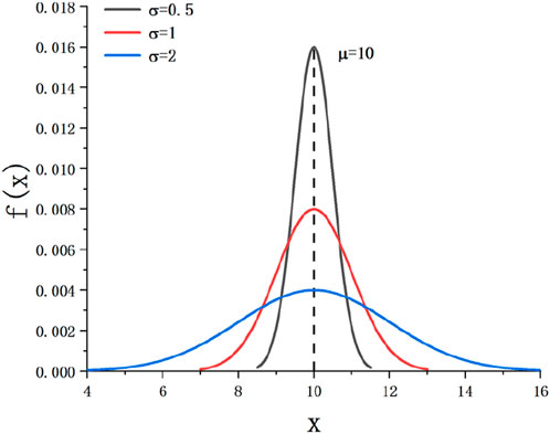
Figure 1. Univariate normal distribution function diagram.

Among them, $\mu$ is the mean, $\sigma$ is the standard deviation.

When considering two Gaussian models simultaneously, the combined bivariate Gaussian model distribution function is shown in Formula 5, and Figure 2 shows the bivariate normal distribution function.

$\begin{array}{ll}\hfill f\left(x_1,x_2\right)& =\frac{1}{2\pi {\sigma }_1{\sigma }_2\sqrt{1-p^2}}\exp \left(-\frac{1}{2\left(1-p^2\right)}\left(\frac{{\left(x_1-{\mu }_1\right)}^2}{{\sigma }_1^2}\right.\right.\hfill \\ \hfill & \left.\left.+|\frac{{\left(x_2-{\mu }_2\right)}^2}{{\sigma }_2^2}|-|\frac{2p\left(x_1-{\mu }_1\right)\left(x_2-{\mu }_2\right)}{{\sigma }_1{\sigma }_2}\right)\right)\hfill \end{array}(5)$

Figure 2

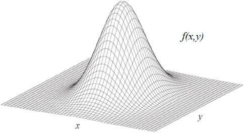
Figure 2. Binary normal distribution function diagram.

Among them, $x_1$ satisfies the normal distribution $\mathrm{N}\left({\mu }_1,{\sigma }_1^2\right)$, $x_2$ satisfies the normal distribution $\mathrm{N}\left({\mu }_2,{\sigma }_2^2\right)$, p is the correlation coefficient, $\mathrm{p}=\frac{C_{12}}{{\sigma }_1{\sigma }_2}$, $C_{12}$ is the covariance, $C_{12}=\mathrm{E}-{\mu }_1{\mu }_2$, and E is the expected value of the binary Gaussian model.

The distribution function of the multivariate Gaussian model is derived analogously, as shown in Formula 6.

$f\left(x_1,x_2,...,x_n\right)=\frac{1}{\sqrt{{\left(2\pi \right)}^n{\left|\mathrm{\Sigma }\right|}^{1/2}}}\exp \left(-\frac{1}{2}{\left(x-\mu \right)}^T{\mathrm{\Sigma }}^{-1}\left(x-\mu \right)\right)(6)$

Among them, $\mathrm{\Sigma }$ is the covariance matrix, $T$ is the transposed symbol, $\mu$ is the mean.

After analyzing the influencing factors of natural gas production, this article uses a multivariate Gaussian mixture model to establish a production planning model. Firstly, establish a single Gaussian model based on each factor, and then use the superposition approach to combine the five Gaussian models together to form a production planning model under multi factor control.

2.3 Production uncertainty prediction model

From the historical production of natural gas, the development of production will go through multiple cycles, with each cycle showing three stages of growth, stability, and decline. Currently, natural gas in the Sichuan Basin is undergoing the fourth production cycle of development. According to the requirements of production planning, under a certain ultimate recoverable reserve URR, the production goes through a growth period, a stable production period, and a decreasing period, with a stable production period of 20 years. Finally, a production planning chart is generated. As shown in Figure 3, based on the historical production data of conventional gas in the Sichuan Basin, boundary conditions are set to predict the development trend of production. From the figure, using the data from 1953 to 2023 as historical data, predictions will be made after 2023, with a production growth period from 2023 to 2032, a stable production period from 2032 to 2051, and a production decline period after 2051. The area of the entire curve is equal to the ultimate recoverable reserve URR.

Figure 3

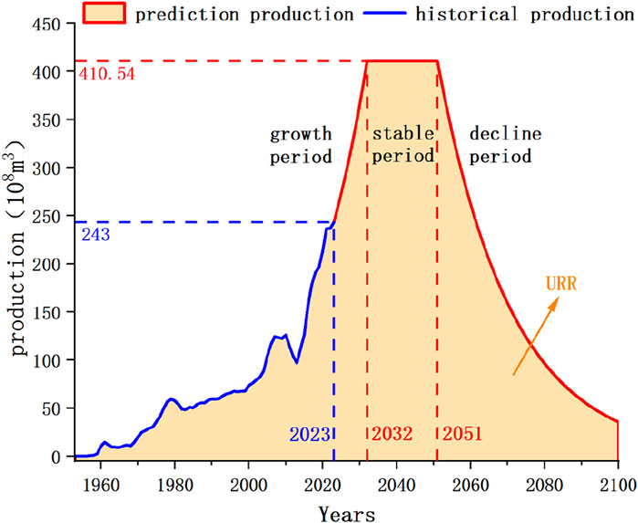
Figure 3. Historical development and production planning curve of conventional gas in Sichuan Basin.

When planning production, it is necessary to consider factors that may affect changes in production. To reasonably screen the influencing factors of production, combined with the production planning chart, starting from different stages of production development, determine the influencing factors. Firstly, during the production growth stage, the production will show different growth rates with changes in the growth rate. Secondly, during the stable production stage, the degree of extraction will also affect the production during the stable production period. Finally, in the stage of production decline, production will show different degrees of decline with changes in the decline rate. In addition, the development of the entire production is also controlled by the ultimate recoverable reserve URR, which is also influenced by the proven rate and recovery rate. In summary, the factors that affect the development of production include the proven rate, recovery rate, growth rate, degree of recovery at the end of stable production period, and decline rate.

By constraining the production and time during the stable production period through these five influencing factors, multiple equations are established, as shown below.

$\left[Q_{ls}+\left(Q+Q_0\right)*\frac{t_m-t_0}{2}\right]+t*Q*c_c+dj*Q=URR(7)$

$\frac{\mathrm{Q}-Q_0}{t_m-t_0}=k*Q_0(8)$

$\text{dj}={\displaystyle \sum _{i=1}^n}{\left(e^{-m}\right)}^i(9)$

$\text{URR}=Q_r*tml*csl(10)$

Among them, $Q$ is the production during the stable production period, and $t_m$ is the time to enter the stable production period. These two variables need to be determined.

$Q_{ls}$ is the historical cumulative production, $Q_0$ is the initial production (predicted from 2024, production in 2023 is $Q_0$), $t_0$ is the time corresponding to the initial production, $t$ is the stable production period years (stable production period of 20 years, $t$ is 20), $i$ is the decreasing period years (decreasing by 50 years, $i$ is 50), $Q_r$ is the resource quantity, all of which are known quantities.

Among them, $tml$ is the proven rate, $csl$ is the recovery rate, $c_c$ is the recovery degree control coefficient, $k$ is the growth rate, and $m$ is the decline rate. These five variables, as risk factors, have an impact on the stable production period $Q$ and the time to enter the stable production period $t_m$ in the production planning model. The final production uncertainty prediction model obtained is as follows.

$Q\left(\mathrm{t}\right)=\left\{\begin{array}{l}{Q}_0*{\left(1+k\right)}^{\left(t-t_0\right)}\left(t_0\le t\le t_m\right)\\ Q\left(t_m\le t\le t_m+19\right)\\ Q*{\left(e^{-m}\right)}^{t-t_m-19}\left(t\ge t_m+19\right)\end{array}\right.(11)$

$\sum Q\left(t\right)+Q_{ls}=URR(12)$

Formula 11 is a production prediction model, where $Q\left(\mathrm{t}\right)$ is the production prediction result, $t$ is the prediction time, $t_0$ is the last year of historical production, $t_m$ is the time of entering the stable production period, $Q_0$ is the production of the last year of historical data, $Q$ is the stable production period production, $k$ is the growth rate, and $m$ is the decreasing rate.

Formula 12 is the model boundary condition, $\sum Q\left(t\right)$ is the cumulative value of production prediction results, and $URR$ is the ultimate recoverable reserves.

3 Analysis of factors affecting production prediction

3.1 Single factor analysis

Based on the historical production data and exploration and development parameters of conventional gas in the Sichuan Basin, an analysis is conducted on five influencing factors: proven rate, recovery rate, growth rate, stable production end recovery degree, and decline rate. The quantitative analysis of production influencing factors requires objective and accurate evaluation of different factors, and requires the generation and calculation of a large amount of factor data. Therefore, the Monte Carlo method is suitable for quantitative research of production influencing factors.

When estimating production probability based on the principle of Monte Carlo method, the problem to be solved must first be transformed into the expected value of a certain probability model. Then, the model is randomly sampled and simulated on a computer to extract sufficient random numbers and perform statistical analysis on the problem to be solved (Li et al., 2022; Simone et al., 2023).

Assuming the distribution density of the known random variable $f\left(x\right)$ is $\psi \left(x\right)$. The mathematical expectation of variable $f\left(x\right)$ is:

$E={\int }_{x_0}^{x_1}f\left(x\right)\psi \left(x\right)dx(13)$

In the formula, $E$ is the expectation, [$x_0$, $x_1$] is the interval of random sampling, and $f\left(x\right)$ is the random variable, $\psi \left(x\right)$ The density function of a random variable.

According to the distribution density function $\psi \left(x\right)$ Randomly select N sample points $x_i$, and use the arithmetic mean of the function value $f\left(x_i\right)$ corresponding to the sample points as the integral estimation value.

$\overline{E_N}=\frac{1}{N}{\displaystyle \sum _{i=1}^N}f\left(x_i\right)(14)$

In the formula, $\overline{E_N}$ is the estimated integral value, $x_i$ is the extracted sample, $f\left(x_i\right)$ is the function value of the extracted sample, and N is the number of samples.

Randomly extract variable values based on the probability distribution density function of the variables. After many independent simulations of the variable values, the probability density distribution of the objective function can be obtained. Monte Carlo simulation can achieve the calculation process of variable random sampling.

In subsequent research, it is necessary to calculate the prediction results and implementation probability of production under different factors, which requires random sampling. Taking the exploration rate as an example, the range of exploration rates is obtained based on actual production, and then a random sampling that conforms to a normal distribution is carried out within the range. 1,000 exploration rates are selected, and the remaining four factors are kept as the average to calculate the production and probability of achievement.

Firstly, the exploration rate and recovery rate are analyzed, both of which directly affect the ultimate recoverable reserve URR of natural gas, thereby affecting the overall amplitude of the production planning model, as shown in Figure 4. As shown in the figure, when other conditions are constant, the larger the ultimate recoverable reserve URR, the greater the production during the stable production period, and the later the time to reach the stable production period. As can be seen from Formulas 7–12, URR is the boundary condition for production prediction, and the result is controlled. Therefore, URR should first be used to study the influence of proved rate and recovery efficiency, and then take them as prior conditions to study other factors by using Bayesian network, to obtain the production prediction results under multi-factor control. In addition, the distribution probability density is calculated by Formulas 13, 14, as shown in the orange bar chart in Figure 5.

Figure 4

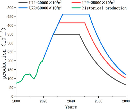
Figure 4. Prediction curves of conventional gas production under different URR conditions.

Figure 5

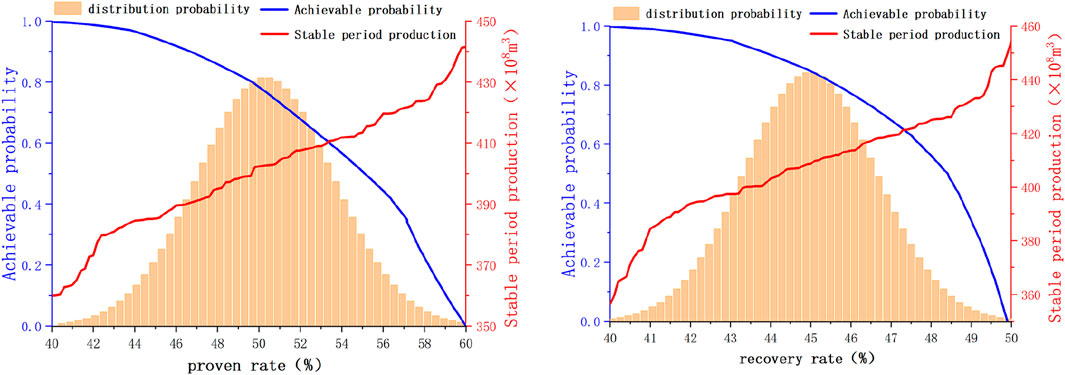
Figure 5. Production probability plots at different proved rates and recovery rates.

The proven rate of conventional gas in the Sichuan Basin is 40%–60%, and the recovery rate is 40%–50%. Under the separate influence of these two factors, the variation of stable production period production with factors and the probability of achievement are shown in Figure 5. From the figure, the production during the stable production period increases with the increase of the proven rate (or recovery rate), but the increase amplitude is inconsistent. The change in production shows a relatively gentle trend in the middle and a sharp change at both ends. This is because after using a normal distribution for Monte Carlo random sampling, within the range of proven rates (or recovery rates), the probability of sampling in the middle is high, while the probability of sampling at both ends is low, resulting in a denser production result in the middle and a looser production result on both sides.

Among them, under the influence of the proven rate, the range of stable production period production is 360–440 $\times {10}^8{m}^3$, and the production is concentrated in 380–420 $\times {10}^8{m}^3$. Under the influence of recovery rate, the range of stable production period production is 355–455 $\times {10}^8{m}^3$, and the production is concentrated in 390–430 $\times {10}^8{m}^3$.

Then analyze the three factors of growth rate, stable production at the end of the period, and decline rate. The trend of changes in the production planning curve and production development probability curve under the separate influence of three factors is shown in Figure 6.

Figure 6

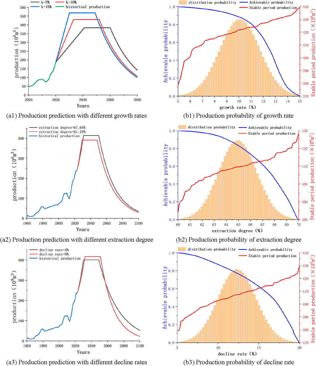
Figure 6. Production prediction curve and Production probability graph under different factors. (A1) Production prediction with different growth rates. (A2) Production prediction with different extraction degree. (A3) Production prediction with different decline rates. (B1) Production probability of growth rate. (B2) Production probability of extraction degree. (B3) Production probability of decline rate.

From Figures 6A1, B1, as the growth rate increases, the increase in production before entering the stable production period increases, and the production will enter the stable production period earlier, and the production during the stable production period is larger. The growth rate of conventional gas is between 5%–15%, and a normal distribution is used for random sampling with a mean of 10%. The range of stable production period production is 380–440 $\times {10}^8{m}^3$, and the production is concentrated in 400–430 $\times {10}^8{m}^3$.

From Figures 6A2, B2, as the degree of recovery at the end of the stable production period increases, the cumulative production at the end of the stable production period is greater, and the production will enter the stable production period later, and the production during the stable production period is greater. The recovery rate at the end of the stable production period is between 60%–70%, and a normal distribution is used for random sampling, with a mean of 65%. The range of production during the stable production period is 385–430 $\times {10}^8{m}^3$, and the production is concentrated in 395–420 $\times {10}^8{m}^3$.

From Figures 6A3, B3, as the decline rate increases, the decrease in production after entering the decline period is greater. Therefore, under other conditions that remain unchanged, the cumulative production before entering the decline period is greater, and the production will enter the stable production period later, and the production during the stable production period is greater. The conventional gas decline rate is around 5%–20%, and a normal distribution is used for random sampling, with an average of 12.5%. The range of stable production period production is 380–430 $\times {10}^8{m}^3$, and the production is concentrated in 390–420 $\times {10}^8{m}^3$.

3.2 Single factor sensitivity analysis

From the content of Section 3.1, different factors have varying degrees of impact on production. Therefore, in subsequent research, it is necessary to first determine the degree of impact of each factor, which requires sensitivity analysis to study the degree of impact of each factor on the production prediction results during the stable production period (Endong et al., 2023; Shuai-hua and Huang, 2020).

Anton Sysoev (Anton, 2023) proposed an alternative method based on finite fluctuation analysis, which obtained a set of sensitivity measures for each input through sensitivity analysis. And the described method was compared with the Sobol index calculation method, proving the consistency of the proposed method. This is a very good sensitivity analysis method, but this article adopts different perspectives for research. This article analyzes the factors that affect production and needs to combine with actual production conditions to study the probability of achieving predicted production. Therefore, the article takes the probability of achieving production as the boundary and studies the maximum and minimum values that can be achieved by a single factor in the range of 0%–100%. The larger the fluctuation range of production, the greater the amplitude and possibility of changes in the actual production process, indicating that production is most sensitive to this factor.

In this section, sensitivity analysis of production prediction results under single factor is carried out, and the research results are as follows. The stable production period production and probability of achievement under different influencing factors are shown in Figure 7. From the perspective of fluctuation range, the proven rate and recovery rate have the greatest impact on the production during the stable production period. The curve changes in the figure show a trend of flat in the middle and steep at both ends, which is also because all factors are randomly sampled using a normal distribution, resulting in concentrated values in the middle and scattered values at both ends.

Figure 7

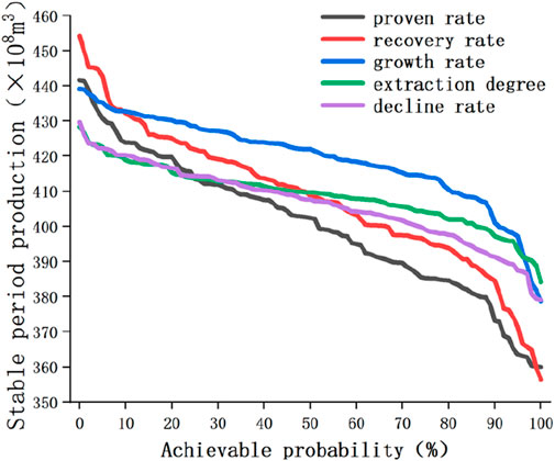
Figure 7. Production probability diagram under different factors.

Sensitivity analysis is conducted based on the production probability graph results of five factors. Since the range of probability of realization is all 0%–100%, the maximum and minimum values of probability are taken to obtain the minimum and maximum production under each influencing factor. Subtraction results in production fluctuations. The larger the fluctuation value, the greater the impact of this factor and the greater its weight. Finally, normalize the production fluctuation value, calculate the weight value, and convert it into a percentage, which is the sensitivity level of the influencing factors, as shown in Table 1.

Table 1

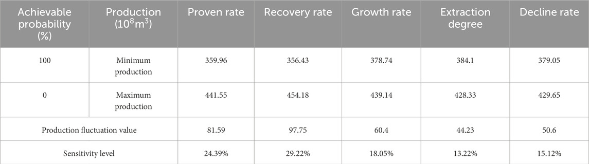
Table 1. Influencing factors sensitivity analysis results table.

The sensitivity level of influencing factors is shown in Figure 8. From the figure, the factors that have a significant impact on the stable production period production are the proven rate, recovery rate, and growth rate, while the factors that have a smaller impact are the extraction degree and decline rate. The sensitivity and weight values of the influencing factors will serve as the basis for subsequent calculations.

Figure 8

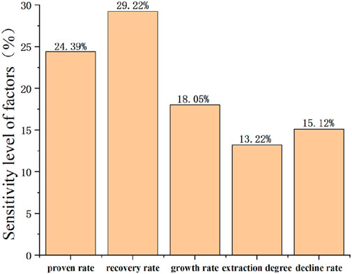
Figure 8. Sensitivity degree diagram of influencing factors.

Based on the analysis of production planning, the target for stable production period production planning of conventional gas is 390 $\times {10}^8{m}^3$. By benchmarking the planned production to the production probability diagram, the predicted range of achievement probability is obtained, as shown in Figure 9. As shown in the figure, the probability range for achieving a stable production period of 390 $\times {10}^8{m}^3$ under five factors is 70%–98%, with a probability greater than 70%, indicating a high possibility of achieving the production planning goal.

Figure 9

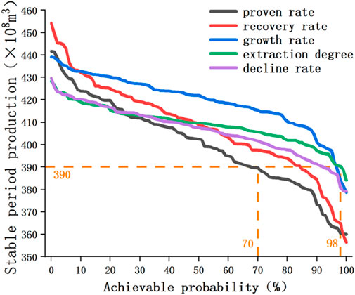
Figure 9. Production probability diagram under different factors.

3.3 Multifactor analysis

After completing the single factor analysis of production, a multi factor analysis of production is carried out by combining Bayesian networks and binary Gaussian models. The specific research ideas are as follows. When conducting multi factor analysis, it is not possible to simultaneously consider the data calculation and graphic drawing of the five factors, therefore, the ultimate recoverable reserve URR is used as the entry point. Firstly, study the impact of the binary probability of proven rate and recovery rate on ultimate recoverable reserve URR and production. Further study the impact of the binary probability generated by the proven rate and recovery rate on production based on the remaining three factors.

In the actual production process, there are many factors that affect natural gas, so it is necessary to study the probability of achieving production during different stable production periods when considering multiple factors at the same time, and develop extraction plans based on the relationship between production and probability. For example, first determine the impact and probability of exploration rate and recovery rate on production, and then combine Bayesian networks to calculate the impact and probability of growth rate, exploration rate and recovery rate on production under the combined effect. Based on the results, determine the appropriate range of growth rate in actual production.

The conventional gas exploration rate in the Sichuan Basin is between 40%–60%, and the recovery rate is between 40%–50%. Due to the normal distribution used for random sampling, the combination of proven rate and recovery rate is also a normal distribution value, with a range of 16%–30%, which means the average is 23%. The conventional gas resource quantity $Q_r=122300\times {10}^8{m}^3$, the range of ultimate recoverable reserve URR is calculated using Formula 9, and the trend of production during stable production period is predicted based on ultimate recoverable reserve URR. The results are shown in Figure 10.

Figure 10

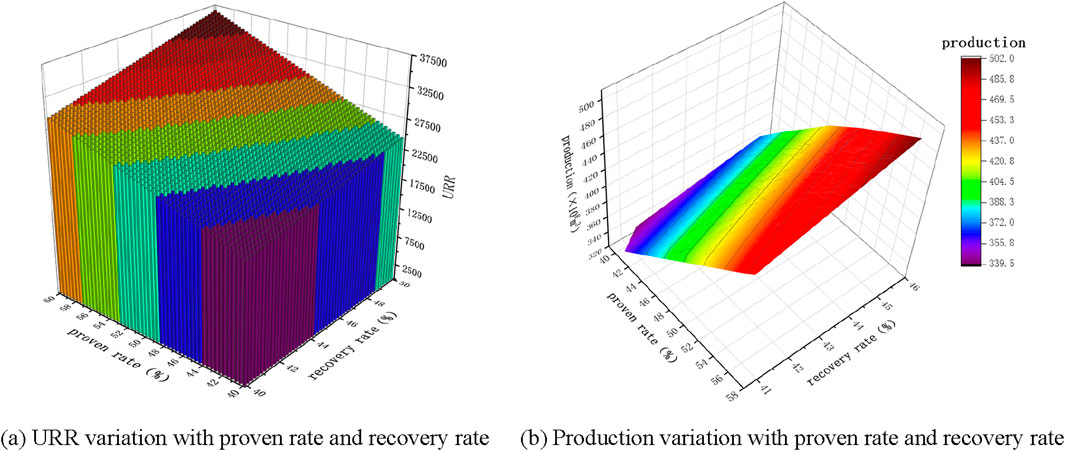
Figure 10. URR and production change trend chart. (A) URR variation with proven rate and recovery rate. (B) Production variation with proven rate and recovery rate.

From Figure 10A, ultimate recoverable reserve URR increases with the increase of proven rate and recovery rate, and the amplitude of change in proven rate has a more significant impact on ultimate recoverable reserve URR. The ultimate recoverable reserve URR range of conventional gas is $19568-36690\times {10}^8{m}^3$. From Figure 10B, the production shows a curved trend with the increase of proved rate and recovery rate, and the overall trend also increases with the increase of proved rate and recovery rate. Under the influence of proven rate and recovery rate, the range of stable production period production is 339–502 $\times {10}^8{m}^3$.

The probability of determining the distribution of proven rate and recovery rate is a normal distribution, with a mean of 23% and a value range of 16%–30%. Using it as a prior probability and other influencing factors as subsequent nodes, establish a Bayesian network and use a binary Gaussian model to calculate the probability of influencing factors.

Take the growth rate as an example to illustrate. The distribution probability of the growth rate is a normal distribution with a mean of 10% and a value range of 5%–15%. As these variables all follow a normal distribution, the Bayesian distribution probability of the growth rate follows a binary normal distribution. Then, the distribution probability is converted into a cumulative probability to obtain the Bayesian implementation probability diagram of the growth rate, as shown in Figure 11. From the figure, when the growth rate, proven rate, and recovery rate are small, the probability of realization is relatively high. As the influencing factors increase, the probability of realization gradually decreases. The probability map of implementation under Bayesian networks will also serve as the basis for the subsequent establishment of multivariate Gaussian mixture models.

Figure 11

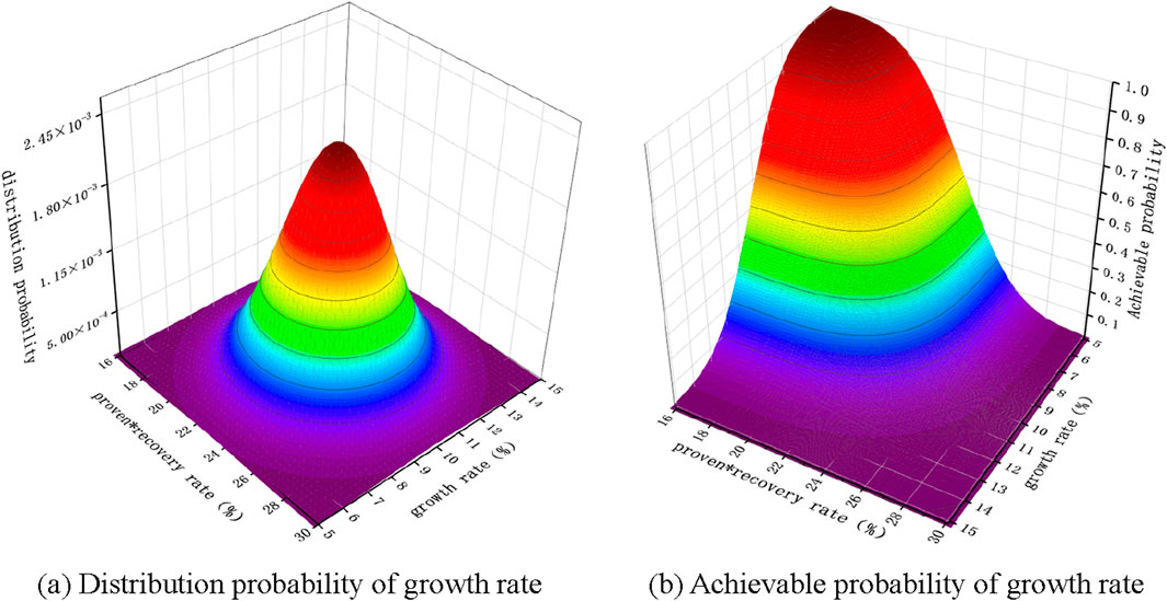
Figure 11. Binary probability plot of growth rate. (A) Distribution probability of growth rate. (B) Achievable probability of growth rate.

Maintain the other influencing factors unchanged, and use Formula 6 to calculate the trend of production changes during the stable production period under the mixed influence of three factors, as shown in Figure 12. From Figure 12A, the trend of production change is an irregular surface graph, and production does not completely increase with the increase of growth rate. It is only a monotonic increasing relationship between production and growth rate within a specific range of proven rate and recovery rate. This pattern can be clearly seen from Figure 12B. Compared with the red and blue lines, when the exploration rate and recovery rate are high, even if the growth rate is low, the stable production period production is relatively high. This is because the production is influenced by a mixture of three factors. In actual production, the range of each factor should be determined based on the production situation, to reasonably control the production. Under the influence of proven rate, recovery rate, and growth rate, the range of stable production period production is 352–500 $\times {10}^8{m}^3$.

Figure 12

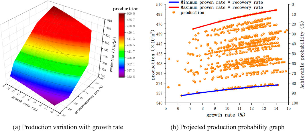
Figure 12. Calculation results under the influence of growth rate. (A) Production variation with growth rate. (B) Projected production probability graph.

Project the three-dimensional production map on the production growth rate surface and combine it with the calculation results of the implementation probability to obtain the production probability map under the Bayesian network. From Figure 12B, the results are shown in the blue curve at the lowest proved recovery rate and the red curve at the highest recovery rate. In the figure, when the stable production period production is about 390 $\times {10}^8{m}^3$, the corresponding probability of achievement is about 70%, while in single factor analysis, the corresponding probability of achievement is 90%. This is because the prior probabilities of proven rate and recovery rate are considered. Currently, under the Bayesian network, the impact of growth rate on production changes, and the probability of achievement decreases, reducing the likelihood of achieving production planning goals.

Similarly, the analysis of extraction degree and decline rate is consistent with the analysis process of growth rate. Using the proven rate and recovery rate as known probabilities, calculate the binary distribution probability of the recovery degree, and then obtain the probability of achieving the recovery degree, as shown in Figure 13A. Finally, combine Formula 6 to calculate the trend of production with the recovery degree, as shown in Figure 13B. The trend of change is an irregular surface graph, which shows that the production does not increase completely with the increase of recovery degree, but only shows a monotonic increasing relationship between production and recovery degree in a specific proved rate recovery rate interval. Under the influence of proven rate, recovery rate, and recovery degree, the range of stable production period production is 376–490 $\times {10}^8{m}^3$.

Figure 13

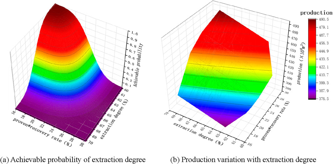
Figure 13. Calculation results under the influence of extraction degree. (A) Achievable probability of extraction degree. (B) Production variation with extraction degree.

Using the proven rate and recovery rate as known probabilities, calculate the binary distribution probability of the decline rate, and then obtain the probability of achieving the decline rate, as shown in Figure 14A. Finally, combine Formula 6 to calculate the trend of production change with the decline rate, as shown in Figure 14B. The trend of change is an irregular surface graph, which shows that production does not increase completely with the increase of decline rate, but only shows a monotonic increasing relationship between production and decline rate in a specific proved rate recovery interval. Under the influence of proven rate, recovery rate, and decline rate, the range of stable production period production is 374–483 $\times {10}^8{m}^3$.

Figure 14

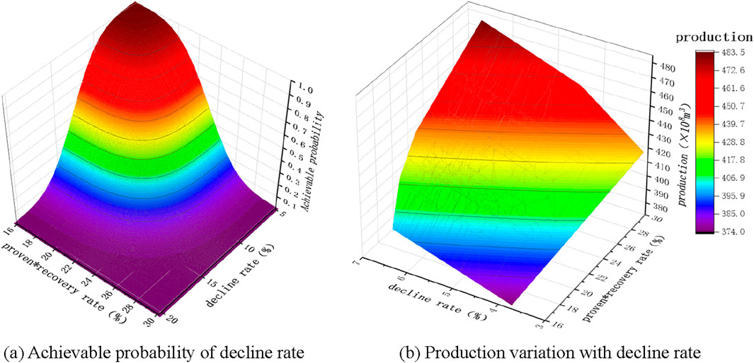
Figure 14. Calculation results under the influence of decline rate. (A) Achievable probability of decline rate. (B) Production variation with decline rate.

3.4 Summary of factor analysis

By conducting a single factor analysis of production, the fluctuation range of influencing factors was determined, and it was clarified that under the influence of a single factor, the stable production period production increased with the increase of influencing factor values. Under the influence of the proven rate, the range of stable production period production is 359.96–441.55 $\times {10}^8{m}^3$; Under the influence of recovery rate, the range of stable production during the production period is 356.43–454.18 $\times {10}^8{m}^3$; Under the influence of growth rate, the range of stable production period production is 378.74–439.14 $\times {10}^8{m}^3$; Under the influence of extraction degree, the range of stable production period production is 384.1–428.33 $\times {10}^8{m}^3$; Under the influence of the decline rate, the range of stable production period production is 379.05–429.65 $\times {10}^8{m}^3$. As shown in Table 2, the recovery rate has the greatest impact on the production, and the degree of recovery has the least impact on the production.

Table 2

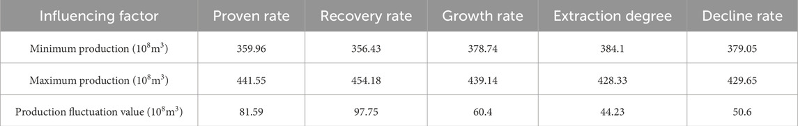
Table 2. Production prediction results table under different factors.

By conducting sensitivity analysis on the factors affecting production, the sensitivity levels of five factors were obtained and converted into weight values for the establishment of subsequent multi factor production planning models. When the production planning target is determined to be 390 $\times {10}^8{m}^3$, the probability of achieving it under the influence of a single factor will exceed 70%, indicating a high possibility of achieving the target production.

By conducting a multifactor analysis of production, the distribution probability of the proven rate and recovery rate was used as a prior probability. The binary distribution probability and implementation probability of the other three factors were calculated, and the trend of stable production period production under the mixed action of multiple factors was predicted. The production during the stable production period does not increase entirely with the increase of influencing factor values, and only within a certain range can this law be met. In addition, taking the production probability projection diagram of growth rate as an example, the variation of stable production period production and its corresponding realization probability under the mixed effects of multiple factors was analyzed. The results showed that compared to the influence of single factors, the probability of achieving production targets under multiple factors decreased. In actual planning, it is necessary to consider the combined effects of multiple factors to more accurately carry out production planning.

4 Establishment of production planning model

Through the previous calculations, the influence law and sensitivity level of a single factor, as well as the probability of achieving mixed effects of multiple factors and the trend of production changes were obtained. Then, based on the sensitivity of a single factor, weight values are assigned to obtain a single factor production planning model. The impact of each factor on production planning is preliminarily analyzed. Finally, a multivariate Gaussian model is used to overlay and combine the single factor production model to obtain a multi factor production planning model.

When establishing a production planning model, it is considered that the greater the impact of a certain factor on production, the higher the proportion of that factor in the model. Therefore, the results of the sensitivity analysis in the previous section are used as weights in the production planning model. According to the sensitivity analysis results in Section 3.2, the sensitivity degree of the influencing factors is converted into weight, and the weight matrix of the five factors, namely, the proven rate, recovery rate, growth rate, recovery degree, and decline rate, is R= [0.25,0.29,0.18,0.13,0.15]. Based on historical data of conventional gas production, allocation is made according to weights, and production planning models are established based on different factors to obtain production prediction curves with different proportions, as shown in Figure 15.

Figure 15

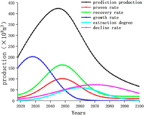
Figure 15. Production prediction curves for different factors.

The black curve in the figure represents the conventional gas production prediction curve, which is composed of five other curves stacked together. The remaining curves represent the production planning model after assigning weights to each of the five factors individually. As shown in the figure, the production curve of growth rate is concentrated in the growth period, the production curve of proven rate and recovery rate is concentrated in the stable production period, and the production curve of recovery degree and decline rate is concentrated in the decline period.

From this, the growth rate affects the trend of production changes during the growth period by controlling the amplitude of growth, and the proven rate and recovery rate affect the overall size of the production prediction curve by controlling the size of ultimate recoverable reserve URR, thereby affecting the trend of production changes throughout the entire life cycle. The most significant impact is the size of production during the stable production period, and the degree of recovery affects the trend of production changes before and after the decline period by controlling the cumulative production at the end of the stable production period, The decline rate affects the trend of production during the decline period by controlling the magnitude of the decline.

Figure 16 shows the trend of production changes under the mixed influence of five factors since 2020, namely, the multi factor production planning chart. The influencing factors of the coordinate axis represent five different factors, from 1 to 5, which are the proven rate, recovery rate, growth rate, extraction degree, and decline rate. As the value of the coordinate axis increases, the factors also overlap and have an impact on the production prediction results. As shown in the figure, the production prediction curve gradually becomes complete with the superposition of influencing factors, and finally forms a production planning curve that includes growth period, stable production period, and decreasing period.

Figure 16

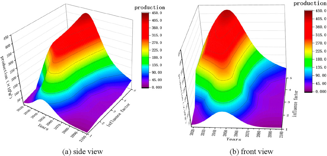
Figure 16. Production planning model under the influence of multiple factors. (A) side view. (B) front view.

From the graph, it can be seen that various factors have an impact on the production planning model. The growth rate controls the amplitude of the production growth stage, the proven rate and recovery rate control the amplitude of the stable production stage, the extraction degree controls the amplitude of the transition from the stable production stage to the decreasing stage, and the decline rate controls the amplitude of the decreasing production stage. Under the combined influence of five factors, the production will reach a peak of 423 $\times {10}^8{m}^3$ in 2045, with a stable production period of 2038–2051. The production planning model can study the forecast results of the production change over time under the influence of different factors, and obtain the influence of each factor on the production at different stages, to better adjust the factors according to the demand in the actual production and achieve the production target.

5 Conclusion

This article establishes a production uncertainty prediction model under multi factor control based on the development of conventional gas production in the Sichuan Basin. By analyzing the factors affecting production, the variation patterns of production and probability of achievement under the influence of single factors were obtained, and the sensitivity levels of different factors were obtained through sensitivity analysis. In addition, a multi factor analysis was conducted based on Bayesian networks, using the detection rate and recovery rate as prior probabilities to obtain binary distribution probabilities and implementation probabilities of other factors, as well as production variation graphs under the influence of multiple factors. A production planning model was established by combining the weight results of the multivariate Gaussian mixture model and sensitivity analysis. The conclusion is as follows.

1) The established production uncertainty model can effectively predict the development trend of production under the control of multiple factors. From the prediction results, production is positively correlated with the five influencing factors of proven rate, recovery rate, growth rate, extraction degree, and decline rate. During the stable production period, production will increase with the increase of the value of the influencing factors, and the degree of influence of the factors from large to small is: recovery rate, recovery rate, growth rate, decline rate, and extraction degree. When the impact of production changes from single factor to multiple factors, the fluctuation range of stable production increases, and the probability of achieving the target production decreases.

2) Based on the weight values of the degree of influence of factors, establish single factor and multi factor production planning models. From the perspective of production development trends, the growth rate controls the amplitude of the production growth stage, the proven rate and recovery rate control the amplitude of the stable production stage, the extraction degree controls the amplitude of the transition from the stable production stage to the decreasing stage, and the decline rate controls the amplitude of the decreasing production stage. These conclusions provide reference for the formulation of production planning goals.

3) Unlike conventional research that considers the impact of a single factor on production, this article comprehensively considers multiple influencing factors, studies the changes in natural gas production, calculates the probability of achieving production, and provides a reference for the formulation of production planning goals. In addition, the article establishes an uncertainty prediction model (Formulas 11, 12), which can effectively combine multiple factors to predict natural gas production.

4) The article analyzes the five main influencing factors of natural gas production, and comprehensive research has certain innovation. However, the influencing factors involved in the research are all those involved in the exploration and development process, and there are also some economic factors (such as investment and cost) that have not been considered. Therefore, more factors can be further considered to analyze the trend of production changes, to develop more suitable production planning schemes.

Data availability statement

The raw data supporting the conclusions of this article will be made available by the authors, without undue reservation.

Author contributions

HL: Conceptualization, Supervision, Writing–original draft, Writing–review and editing. GY: Data curation, Methodology, Supervision, Writing–review and editing. YF: Methodology, Validation, Writing–original draft. YaC: Supervision, Validation, Writing–original draft. KS: Investigation, Methodology, Writing–review and editing. YL: Methodology, Validation, Writing–review and editing. YuC: Investigation, Methodology, Validation, Writing–original draft. DZ: Methodology, Supervision, Validation, Writing–original draft, Writing–review and editing.

Funding

The author(s) declare that no financial support was received for the research, authorship, and/or publication of this article.

Conflict of interest

Authors HL, YF, YaC, and YL were employed by Exploration and Development Research Institute of PetroChina Southwest Oil and Gas Field Company.

Author GY was employed by PetroChina Southwest Oil and Gas Field Company Planning Department.

The remaining authors declare that the research was conducted in the absence of any commercial or financial relationships that could be construed as a potential conflict of interest.

Publisher’s note

All claims expressed in this article are solely those of the authors and do not necessarily represent those of their affiliated organizations, or those of the publisher, the editors and the reviewers. Any product that may be evaluated in this article, or claim that may be made by its manufacturer, is not guaranteed or endorsed by the publisher.

References

Adriana, L.L.-L., and Martha, L. (2021). Fitting a Gaussian mixture model through the gini index. Int. J. Appl. Math. Comput. Sci. 31, 487–500. doi:10.34768/amcs-2021-0033

CrossRef Full Text | Google Scholar

Andreas, W. (2021). Quantum-like Gaussian mixture model. Soft Comput. 25, 10067–10081. doi:10.1007/s00500-021-05941-9

CrossRef Full Text | Google Scholar

Anton, S. (2023). Sensitivity analysis of mathematical models. Computation 11, 159. doi:10.3390/computation11080159

CrossRef Full Text | Google Scholar

Arun Kumar, S., Erfan, B. T., Alireza, G., and Dehnavi-Arani, S. (2020). Robust optimization and mixed-integer linear programming model for LNG supply chain planning problem. Soft Comput. 24, 7885–7905. doi:10.1007/s00500-019-04010-6

CrossRef Full Text | Google Scholar

Bilici, Z., Özdemir, D., and Temurtaş, H. (2023). Comparative analysis of metaheuristic algorithms for natural gas demand forecasting based on meteorological indicators. J. Eng. Res. 11, 259–265. doi:10.1016/j.jer.2023.100127

CrossRef Full Text | Google Scholar

Cangqi, Z., Hao, B., Jing, Z., Li, Q., and Zhang, Y. (2020). Gaussian mixture variational autoencoder for semi-supervised topic modeling. IEEE ACCESS 8, 106843–106854. doi:10.1109/access.2020.3001184

CrossRef Full Text | Google Scholar

Chen., Q., Zhang., Z., Chunming, F., Hu, D., and Jiang, C. (2024). Enhanced Gaussian-mixture-model-based nonlinear probabilistic uncertainty propagation using Gaussian splitting approach. Struct. Multidiscip. Optim. 67, 49. doi:10.1007/s00158-023-03733-3

CrossRef Full Text | Google Scholar

Chong, L., Tongfei, L., Wen-Ze, W., Xie, W., and Zhu, H. (2022). An optimized nonlinear grey Bernoulli prediction model and its application in natural gas production. Expert Syst. Appl. 194, 116448. doi:10.1016/j.eswa.2021.116448

CrossRef Full Text | Google Scholar

Chunsheng, G., Jialuo, Z., Huahua, C., Ying, N., Zhang, J., and Zhou, D. (2020). Variational autoencoder with optimizing Gaussian mixture model priors. IEEE ACCESS 8, 43992–44005. doi:10.1109/access.2020.2977671

CrossRef Full Text | Google Scholar

David, A., Concha, B., and Pedro, L. (2022). Semiparametric bayesian networks. Inf. Sci. 584, 564–582. doi:10.1016/j.ins.2021.10.074

CrossRef Full Text | Google Scholar

Deyan, W., Adam, A. J., and Ying, X. (2020). Dynamic knowledge inference based on bayesian network learning. Math. Problems Eng. 2020, 6613896. doi:10.1155/2020/6613896

CrossRef Full Text | Google Scholar

Dongfeng, L., Heng, F., Wang, R., Yang, S., Zhao, Y., and Yan, X. (2022). Prediction of casing collapse strength based on bayesian neural network. Processes 10, 1327. doi:10.3390/pr10071327

CrossRef Full Text | Google Scholar

Durmuş, Ö., Safa, D., Doğan, A., et al. (2022). A new modified artificial bee colony algorithm for energy demand forecasting problem. Neural Comput. Appl. 34, 17455–17471. doi:10.1007/s00521-022-07675-7

CrossRef Full Text | Google Scholar

Duygu, I., and Derya, E. (2019). A new approach for probability calculation of fuzzy events in Bayesian Networks. Int. J. Approx. Reason. 108, 76–88. doi:10.1016/j.ijar.2019.03.004

CrossRef Full Text | Google Scholar

Endong, W., Lianjun, Z., Hong, C., and Zhang, X. (2023). Collinearity-oriented sensitivity analysis for patterning energy factor significance in buildings. J. Build. Eng. 73, 106685. doi:10.1016/j.jobe.2023.106685

CrossRef Full Text | Google Scholar

Erick, M., Fernando, L. C. O., and de Menezes, L. M. (2022). Forecasting natural gas consumption using Bagging and modified regularization techniques. Energy Econ. 106, 105760. doi:10.1016/j.eneco.2021.105760

CrossRef Full Text | Google Scholar

Guo, Yu., Haitao, Li., Yanru, C., Liu, L., Wang, C., Chen, Y., et al. (2021). Quantitative study on natural gas production risk of Carboniferous gas reservoir in eastern Sichuan. J. Petroleum Explor. Prod. Technol. 11, 3841–3857. doi:10.1007/s13202-021-01261-8

CrossRef Full Text | Google Scholar

Haitao, L., Guo, Y., Chen, Y., and Zhang, D. (2021). Research on quantitative evaluation methods and influencing factors of natural gas reservoir development. Shock Vib. 2021, 1684178. doi:10.1155/2021/1684178

CrossRef Full Text | Google Scholar

Haoran, L., Shaopeng, C., Sheng, L., Wang, N., Shi, Q., Cai, Y., et al. (2022). A bayesian network structure learning algorithm based on probabilistic incremental analysis and constraint. IEEE ACCESS 10, 130719–130732. doi:10.1109/access.2022.3229128

CrossRef Full Text | Google Scholar

Hongbing, L., and Han, M. (2023). Forecast of China’s natural gas demand based on the double-logarithmic model with stepwise regression method. Energy Policy 45, 8491–8506. doi:10.1080/15567036.2023.2227584

CrossRef Full Text | Google Scholar

Jian, C., Ting, L., Lai, K. K., Zhang, Z. G., and Wang, S. (2018). The future natural gas consumption in China: based on the LMDI-STIRPAT-PLSR framework and scenario analysis. Energy Policy 119, 215–225. doi:10.1016/j.enpol.2018.04.049

CrossRef Full Text | Google Scholar

Jianliang, W., and Nu, L. (2020). Influencing factors and future trends of natural gas demand in the eastern, central and western areas of China based on the grey model. Nat. Gas. Ind. B 7, 473–483. doi:10.1016/j.ngib.2020.09.005

CrossRef Full Text | Google Scholar

Jianzhong, X., Xiaolin, W., and Wang, R. (2016). Research on factors affecting the optimal exploitation of natural gas resources in China. Sustainability 8, 435. doi:10.3390/su8050435

CrossRef Full Text | Google Scholar

Jiří, V., Václav, K., and Kratochvíl, F. (2023). Structural learning of mixed noisy-OR Bayesian networks. Int. J. Approx. Reason. 161, 108990. doi:10.1016/j.ijar.2023.108990

CrossRef Full Text | Google Scholar

Joachim, G., Philipp, L., Linda, P., Schmalwasser, L., and Lawonn, K. (2024). The whole and its parts: visualizing Gaussian mixture models. Vis. Inf. 8, 67–79. doi:10.1016/j.visinf.2024.04.005

CrossRef Full Text | Google Scholar

Julie, D., and Agnes, D. (2020). A wasserstein-type distance in the space of Gaussian mixture models. SIAM J. Imaging Sci. 13, 936–970. doi:10.1137/19m1301047

CrossRef Full Text | Google Scholar

Jun, L., Yan-Bin, Y., and Derek, E. (2024). Morphological complexity and azimuthal disorder of evolving pore space in low-maturity oil shale during in-situ thermal upgrading and impacts on permeability. Petroleum Sci. doi:10.1016/j.petsci.2024.03.020

CrossRef Full Text | Google Scholar

Kyung, B., Soo, H. L., Yoon, H. J., Park, H., Kim, J., Cheong, S., et al. (2024). Implementation of Bayesian networks and Bayesian inference using a Cu_0.1Te_0.9/HfO₂/Pt threshold switching memristor. Nanoscale Adv. 6, 2892–2902. doi:10.1039/d3na01166f

PubMed Abstract | CrossRef Full Text | Google Scholar

Li, H., Yu, G., Fang, Y., Chen, Y., and Zhang, D. (2022). Studies of natural gas production prediction and risk assessment for tight gas in Sichuan Basin. Front. Earth Sci. 10, 1059832. doi:10.3389/feart.2022.1059832

CrossRef Full Text | Google Scholar

Luca, S. (2023). Entropy-based anomaly detection for Gaussian mixture modeling. Algorithms 16, 195. doi:10.3390/a16040195

CrossRef Full Text | Google Scholar

Marta, M., Gregorio, F. V., Alicja, K., Wodarski, K., and Riesgo Fernández, P. (2020). Optimizing predictor variables in artificial neural networks when forecasting raw material prices for energy production. Energies 13, 2017. doi:10.3390/en13082017

CrossRef Full Text | Google Scholar

Maruf, G. (2021). A novel approach for Gaussian mixture model clustering based on soft computing method. IEEE ACCESS 9, 159987–160003. doi:10.1109/access.2021.3130066

CrossRef Full Text | Google Scholar

Nuo, W., Yuxiang, Z., Tao, S., Zou, X., Wang, E., and Du, S. (2022). Accounting for China’s net carbon emissions and research on the realization path of carbon neutralization based on ecosystem carbon sinks. Sustainability 14, 14750. doi:10.3390/su142214750

CrossRef Full Text | Google Scholar

Özdemir, D., Dörterler, S., and AydinDo, D. (2022). An adaptive search equation-based artificial bee colony algorithm for transportation energy demand forecasting. Turkish J. Electr. Eng. Comput. Sci. 30, 1251–1268. doi:10.55730/1300-0632.3847

CrossRef Full Text | Google Scholar

Palanisamy, M., Md, S. A., Majed, A., Khan, U., Alagirisamy, K., Pachiyappan, D., et al. (2021). Forecasting natural gas production and consumption in United States-evidence from SARIMA and SARIMAX models. Energies 14, 6021. doi:10.3390/en14196021

CrossRef Full Text | Google Scholar

Qi, Z., Chunjie, Z., Yu-Chu, T., Xiong, N., Qin, Y., and Hu, B. (2018). A fuzzy probability bayesian network approach for dynamic cybersecurity risk assessment in industrial control systems. IEEE Trans. INDUSTRIAL Inf. 14, 2497–2506. doi:10.1109/tii.2017.2768998

CrossRef Full Text | Google Scholar

Shuai-hua, Ye., and Huang, A. (2020). Sensitivity analysis of factors affecting stability of cut and fill multistage slope based on improved grey incidence model. Soil Mech. Found. Eng. 57, 8–17. doi:10.1007/s11204-020-09631-w

CrossRef Full Text | Google Scholar

Simone, C., Jeanne, T., Martin, W., and Zamponi, F. (2023). Machine-learning-assisted Monte Carlo fails at sampling computationally hard problems. Mach. Learn. Sci. Technol. 4, 010501. doi:10.1088/2632-2153/acbe91

CrossRef Full Text | Google Scholar

Song, Y., Dongzhao, Y., Wei, S., Deng, C., Chen, C., and Feng, S. (2023). Global evaluation of carbon neutrality and peak carbon dioxide emissions: current challenges and future outlook. Environ. Sci. Pollut. Res. 30, 81725–81744. doi:10.1007/s11356-022-19764-0

CrossRef Full Text | Google Scholar

Tongfei, L., and Yanrui, S. (2022). Predicting the production and consumption of natural gas in China by using a new grey forecasting method. Math. Comput. Simul. 202, 295–315. doi:10.1016/j.matcom.2022.05.023

CrossRef Full Text | Google Scholar

Wang, Y., Chen, Q., Dai, B., and Wang, D. (2024). Guidance and review: advancing mining technology for enhanced production and supply of strategic minerals in China, Green and Smart Mining. Engineering 1, 2–11. doi:10.1016/j.gsme.2024.03.005

CrossRef Full Text | Google Scholar

Yang, D., Jingliang, D., Tonglin, Y., Zhou, S., and Wei, Y. (2021). Failure evaluation of bridge deck based on parallel connection bayesian network: analytical model. Materials 14, 1411. doi:10.3390/ma14061411

PubMed Abstract | CrossRef Full Text | Google Scholar

Yaser, S., Parvin, N., Iraj, M., and Azam, K. (2021). Predicting the probability of occupational fall incidents: a Bayesian network model for the oil industry. Int. J. Occup. Saf. Ergonomics 27, 654–663. doi:10.1080/10803548.2019.1607052

CrossRef Full Text | Google Scholar

Yingying, X., Xiangui, L., Zhiming, H., Shao, N., Duan, X., and Chang, J. (2022). Production effect evaluation of shale gas fractured horizontal well under variable production and variable pressure. J. Nat. Gas Sci. Eng. 97, 104344. doi:10.1016/j.jngse.2021.104344

CrossRef Full Text | Google Scholar

Zhe, G., Zhaochen, S., and Shuxiu, L. (2020). Probability density function for wave elevation based on Gaussian mixture models. Ocean. Eng. 213, 107815. doi:10.1016/j.oceaneng.2020.107815

CrossRef Full Text | Google Scholar