Robustness of characteristics of the Matuyama-Brunhes geomagnetic field reversal found in global models

Paleomagnetic data enables the global reconstruction of the geomagnetic field, allowing the investigation of significant events like polarity reversals and excursions. When compared to prior polarity reversals, the most recent one, the Matuyama-Brunhes (MB), is the best recorded reversal in terms of number of available paleomagnetic data. Nevertheless, several of these data have poor age control, and they are not distributed equally worldwide. Few global models have been presented for the MB; the most recent is the GGFMB (Global Geomagnetic Field Model for the MB reversal). Limitations imposed by input data and subjective assumptions about the data that are made in modelling restrict the resolution and reliability of these models. This study presents a suite of eight additional global models that reconstruct the magnetic field during the interval 700–900 ka ago, including the MB reversal and Kamikatsura (KKT) excursion. Through model comparisons, the robustness of the models in resolving MB reversal characteristics is assessed. The majority of models indicate that the reversal was mainly driven by the axial dipole field contribution gradually decreasing, while non-dipole parts slightly increased. At the core-mantle boundary, two high-latitude reverse flux patches appear at the beginning of the reversal, and it seems like a few precursors in the form of regionally seen transitional field occurred, related to variations in the decaying dipole moment. The main global polarity change occurred close to 778 ka, with the axial dipole quickly strengthening in the opposite direction in the following, completing the full polarity transition. All the models confirm the previously reported asymmetry of slow dipole decay and fast recovery, and indicate that the dipole moment was clearly lower in the late Matuyama than the early Brunhes. The whole reversal process occurred on average between 800 and 770 ka, with a duration of approximately 30 kyr. Out of four apparent excursions discovered in some of the models between 900 and 800 ka, the KKT excursion (890–884 ka), can be confirmed as a robust magnetic field feature. Additional, well dated paleomagnetic records in particular from the southern hemisphere are required to confirm several details suggested by the models that should only be interpreted with caution so far.

1 Introduction

The geomagnetic field, generated and maintained by dynamo activity in the Earth’s core, varies continuously. The most extreme changes are full polarity reversals. Throughout Earth’s history, numerous, sporadic magnetic reversals occurred (Cande and Kent, 1995; Channell et al., 2020; Ogg, 2020), which can be described as transitions between two quasi-stable polarity chron states. Reversals are associated with a collapse of the geomagnetic dipole field (Van Zijl et al., 1962; Singer et al., 2019), resulting in an increase in the atmospheric generation of cosmogenic nuclide particles (Elsasser et al., 1956; Simon et al., 2019). Most of the paleomagnetic data documenting reversals come from volcanic and sediment records. Matuyama-Brunhes (MB) is the most recent field reversal, studied by tens of these records. However, previous studies that assembled and assessed the MB database demonstrate that MB data are not distributed evenly over the globe (Love and Mazaud, 1997; Singer et al., 2019; Mahgoub et al., 2023a), and a significant number of the sediment records lack precise chronological information.

High-resolution sediments are essential for tracking changes in the Earth’s magnetic field during the polarity change. However, the quality of the recording varies due to several factors, such as the processes involved in acquiring the remanent magnetization, sedimentation rate (Roberts and Winklhofer, 2004; Channell, 2017) and its continuity or interruption, the lock-in effect (Lund and Keigwin, 1994; Channell et al., 2004; Sagnotti et al., 2005), and the sampling type, i.e., whether it is discrete or U-channels (Nagy and Valet, 1993; Roberts, 2006; Sagnotti et al., 2016). Taken together, these factors imply that many sediment records are unlikely to reflect fast oscillations in the magnetic field (that happen on sub-millennial to centennial periods, as might be relevant during reversals) (Roberts and Winklhofer, 2004; Roberts, 2015; Valet and Fournier, 2016; Channell, 2017; Sagnotti, 2018). Volcanic records, on the other hand, provide only sparse and discontinuous paleomagnetic results (Balbas et al., 2018; Singer et al., 2019).

Global models based on spherical harmonics basis functions can be used to study characteristics of the global reversal process, hence providing insights into the underlying mechanism. Few models have been created so far for the MB (Shao et al., 1999; Leonhardt and Fabian, 2007; Ingham and Turner, 2008; Mahgoub et al., 2023b). Using four records—three from the North Atlantic and one volcanic record from La Palma—Leonhardt and Fabian (2007) constructed the IMMAB4 model. Ingham and Turner (2008) used 11 records, half of which from around the Atlantic (see Figure 2 in Mahgoub et al. (2023b)), to built a model which we label IT08. Both models span only the time from beginning to end of the reversal. The GGFMB (global geomagnetic field model for the Matuyama-Brunhes) model was developed by Mahgoub et al. (2023b) utilising 38 sediment records, and encompasses the much longer time from 900 to 700 ka, including stable field phases of the late Matuyama and early Brunhes. Although the global distribution of GGFMB records is better than that of IMMAB4 and IT08, data from the southern and western hemispheres are still few. These models have been used to investigate the evolution of dipole and non-dipole field contributions during the reversal, as well as the morphology of the magnetic field at core-mantle boundary and at the Earth’s surface. However, the resolution and accuracy of the MB models are limited by the issues of the available MB data as noted above.

When constructing global models for the MB reversal, like GGFMB, several subjective choices have to be made. These relate mainly to data selection and pre-processing, but also to the regularization parameters. In this study, a set of eight additional global models has been constructed for the MB reversal that covers the interval 700–900 ka. In addition to the MB reversal, this time interval includes the Kamikatsura (KKT) excursion, dated around 888 ka (Mahgoub et al., 2023b). The data sets for the new models are aimed at exploring a range of subjective choices regarding the data. They are modifications and subsets of that used for the GGFMB model, that have been classified according to geographic distribution, timescale reliability, temporal resolution, and type, as described in Section 2. The modelling method is also outlined there. By comparing all models including GGFMB (Section 3) we assess how robustly these models can resolve characteristics of the MB reversal. Our robust findings about the reversal are summarized in the conclusions in Section 4. “Robust” in this context means, that the results do not depend on the subjective choices made during the modeling. This concept of robustness does not allow quantitative evaluation, which is beyond the scope of this study. Statistical limitations of the pursued inversion techniques and inherent, statistically not well understood uncertainties in data and age models further hamper quantitative analysis.

2 Data and methods

2.1 Input data sets

The paleomagnetic data spanning the interval 700–900 ka ago used in this study are the 68 sediment records compiled and processed by Mahgoub et al. (2023a), distributed mainly on the northern hemisphere. Also, volcanic (lava) data with radiometric dates (⁴⁰Ar/³⁹Ar and K-Ar) were included from 10 regions which are distributed mainly in the western hemisphere. Paleomagnetic data available only on depth-scale without age information and data acquired from loess deposits were not included.

From the 68 records, Mahgoub et al. (2023b) used 38 sediment records as input for constructing the GGFMB model. Most of these records have independent age data, and their paleomagnetic direction and/or relative paleointensity (RPI) demonstrate an acceptable degree of regional consistency with adjacent records [for more details see Mahgoub et al. (2023a)]. We considered the input data of GGFMB as the primary data set, from which we constructed eight additional data sets: G-ALI, G-STA, G-SEL, G-VOL, G-CMP, G-LSR, G-IND1, and G-IND2. The geographical distribution of these data sets is depicted in Figure 1, and their primary characteristics and differences are described below and listed in Table 1. Supplementary Material S1 contains detailed information about each data set and a table indicating which records are included in each data set, respectively.

Figure 1

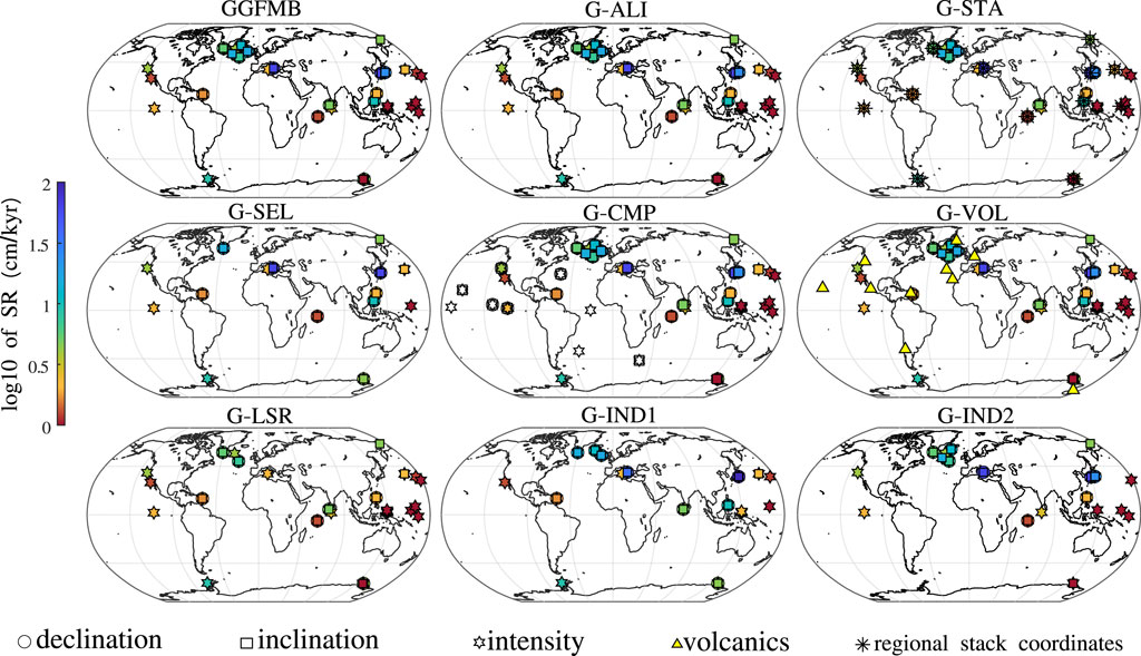
Figure 1. Geographic distribution of the nine input data sets for the models of this study. The primary data set is the one used for model GGFMB (Mahgoub et al., 2023a), of which the other eight are modifications or subsets. The GGFMB data set consists of 38 records indicated by colored circles, squares and stars. The sedimentation rate (SR) of these records is shown using a logarithmic colour scale. The open symbols in G-CMP denote additional sediment records; and the triangles volcanic data in G-VOL, that all have not been used in GGFMB. (See main text for more details).

Table 1

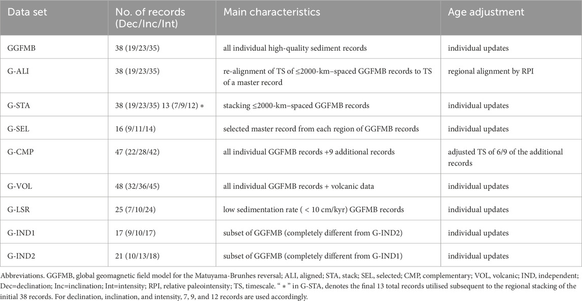
Table 1. Characteristics of the data sets used for modelling the Matuyama-Brunhes reversal.

Dating uncertainties can be large and inconsistent ages of adjacent records may lead to artificial structure in a resulting model. Hence, the G-ALI (aligned) data set contains the same records as GGFMB (Figure 1), but the timescale (TS) of records that are located in close proximity within one region are aligned with the TS of a master record for the region. This master record was selected based on the quality of the applied dating method, the temporal resolution, and sufficient length of the record. The scaled intensity is used for TS alignment, arguing that the minimum intensity during the reversal should occur at similar times in the same region. The alignment was achieved by simply shifting the scaled intensity TS of a record to match the TS of the intensity minimum of the master record. When declination and inclination records existed from the same location, their timescales were shifted along with the intensity component. The regional alignment is conducted on eight regions that contain at least 2 records within an area of radius $\le$1,000 km. These are the North Atlantic, Western Equatorial Pacific (West Caroline Basin), Western Equatorial Pacific (Melanesia Basin), North Pacific (Japan), North Pacific (Hess Rise), Mediterranean, Equatorial Indian Ocean, and Eastern North Pacific. Supplementary Material S1 contains a list of data records in each of these regions, as well as details about the selected master record. Two nearby records exist in the East-Wilkes Basin (Antarctica) region; however, a meaningful correlation of the two high and low resolution records was not possible (see the Supplementary Material S1; Supplementary Figure S9 for further details). The paleomagnetic time series before and after the regional alignment in each of the eight regions are depicted in Supplementary Figures S1–S8. G-ALI additionally includes the individual records from the West Wilkes Basin in Antarctica, the Eastern Equatorial Pacific, the Caribbean Sea and the Russian Arctic that were also used in GGFMB.

The G-STA (stack) data set is constructed by regional stacking of the 38 GGFMB records in nine regions, so that each region is represented by only one representative record in the modelling. Declination, inclination, and intensity data were compiled for nine regions that include at least two sediment records (as specified in G-ALI). All directional and intensity data from the same region were relocated by virtual geomagnetic pole (Noel and Batt, 1990) and virtual axial dipole moment (Creer et al., 1983), respectively, to the geographic coordinates of the master record for this region in order to mitigate the influence of latitude. Using the bootstrapping technique described in Mahgoub et al. (2023a), 5,000 realisations were generated for each of the relocated records. The individual components of these realisations undergo a smoothing spline fit, from which an average fit is derived and generated every 500 years. This average represents the regional stack. The nine regional stacks are shown in the Supplementary Figures S10–S18. In order to carry out the relocation procedure, it is necessary to have both declination and inclination data available simultaneously. However, this requirement is not met for three records (U1304, PC20, SO202-1; See Supplementary Material S1.2; Supplementary Table S1) where declination is not available. In these cases, the declination data were assigned fixed values of 0° and 180° throughout the reverse and normal polarity chron periods, respectively. It should be noted that relocation methods are based on the assumption of a dipolar field configuration, which is not applicable during periods of a magnetic field reversal, but with the rather small relocation distances, the influence of this false assumption is small compared to other uncertainties. G-STA additionally includes the four individual records as G-ALI. Note that TS of the individual records were not aligned prior to establishing regional stacks, but we kept the individual age data as used for GGFMB.

As can be seen in Figure 1, records of GGFMB are concentrated spatially on the Northern hemisphere, mainly in the regions of North Atlantic, Western Equatorial Pacific, and North Pacific. As an alternative to regional stacking, we also included a data set, G-SEL, where one representative record is chosen from each of the well covered regions. The records, selected for good quality, are identical to the master records of G-ALI and re-locations centers of G-STA. Only when the selected master record does not cover the entire time of interest or lacks complete vector information, we expanded it by a nearby high quality record. For example, this was done in the Mediterranean region, where the G-ALI reference record, HS (Sagnotti et al., 2014; Sagnotti et al., 2016), only encompasses a time period of 13 kyrs (780–793 ka). For the period before and after, we used the longest (though lowest resolution) record LC07 (Dinarès-Turell et al., 2002), as noted in Supplementary Table S1. The G-SEL data set consists of 16 records without any TS alignment.

G-CMP (Figure 1) is a complementary data set that supplements the GGFMB records with additional sediment records to improve the spatial data coverage compared to GGFMB. These records were not used for GGFMB because they did not have independent age information, but were dated only by the correlation to a polarity timescale. The nine additional records are from regions of the Atlantic, Pacific, and southern Africa (Figure 1). Declination adjustment and RPI calibration were done in the same way as for the GGFMB records (Mahgoub et al., 2023a). Considering that the additional records have no age information independent of the geomagnetic field, we compared them to the GGFMB predictions for the same locations and adjusted their TS by correlation to the model curve in the cases where clear discrepancies were found. Six out of nine of these records were adjusted in this way, while the remaining three were used on their original TS (see Supplementary Material S1 for more information). Note that this TS adjustment obviously means that the additional information we have added is not fully independent from the GGFMB model.

The data set labelled G-VOL includes volcanic data from 10 regions along with the GGFMB records. The volcanic data consist of 107 site-mean declinations and inclinations and 42 site-mean paleointensities. This volcanic data set is described in detail by Mahgoub et al. (2023a) and the locations are indicated in Figure 1.

G-LSR is created from low sedimentation rate (SR) GGFMB records to see how much information we loose in the model in that case. All sediment records of SR $<$ 10 cm/kyr are considered in G-LSR. This applies to 25 sediment records, of which 7 have declination, 10 inclination, and 24 intensity. Differences to the GGFMB dataset actually mainly affect the North Atlantic and Japan, where five high resolution records were omitted in both these regions.

Finally, two independent (IND) data sets, data G-IND1 and G-IND2, were constructed by using about half of the GGFMB records in each, with as good as possible global distribution. While each of these data sets might lack some regional information, they will lend high credibility to magnetic field features that are found similarly in two models based on information independent from each other. The records included in G-IND1 and G-IND2 are depicted in Figure 1 and listed in Supplementary Table S1.

2.2 Modelling method

Our new models were built using same regularized methodology that has been used in the construction of the GGFMB model (Mahgoub et al., 2023b) and follows the modelling of millennia-scale field models (e.g., CALSxk (Korte et al., 2009; Constable et al., 2016) and GGF100k (Panovska et al., 2018)). The inversion is based on spherical harmonic functions (up to degree 6) in space and cubic B-splines (with 200-year knot point spacing) for the Gauss coefficients in time. The misfit to the data is measured by the L2 norm, and regularizations in space and time were done using quadratic norms (Whaler and Gubbins, 1981; Gubbins, 1983). These allow for the determination of the spatial and temporal resolution of the model by balancing the complexity of the model with its fit to data. In this study, the spatial $({\lambda }_S)$ and temporal $({\lambda }_T)$ regularisation parameters were established based on trade-off curves (Gubbins, 2004; Panovska et al., 2018), which compare the L2 misfit with the spatial $(\mathrm{\Psi })$ and temporal $(\mathrm{\Phi })$ complexity of the model.

The data are weighted using the same methodology as for the GGFMB model. We give equal weight to all sediment data by assigning ${\alpha }_{95}$ of 8.5° for directions and 5 $\mu$T for intensity values. Due to the small number of volcanic data compared to the sediments, we assigned larger weights to these additional data in the G-VOL data set by reducing these values to ${\alpha }_{95}$ of 3.0° and intensity weights to 1 $\mu$T. The ${\alpha }_{95}$ were converted to standard deviation of declination and inclination (Suttie and Nilsson, 2019). For GGFMB, Mahgoub et al. (2023b) had used inclination values calculated from a geocentric axial dipole. Here, we tested using the actual inclination values when they were available. However, as we found essentially no difference to the modelling results between the two methods we kept the previous approach. An iterative data rejection of data falling outside of 10 standard deviations of the model was applied. See Mahgoub et al. (2023b) for more details about the modelling method.

3 Results and discussion

3.1 New global models for the past 700–900 ka

Eight new global paleomagnetic field models (G-ALI, G-STA, G-SEL, G-CMP, G-VOL, G-LSR, G-IND1, and G-IND2), named after their corresponding data sets were constructed in this study. Table 2 includes: the total amount of input data as well as the number of individual magnetic field components (declination, inclination, and intensity), root mean square (rms) misfit of the models (normalised by the data weights) to the whole data set and the individual components, the regularization parameters (${\lambda }_S$ and ${\lambda }_T$), and the spatial $(\mathrm{\Psi })$ and temporal $(\mathrm{\Phi })$ complexity of the models. The parameters of the main model, GGFMB, are given as well. Additional information about the new models is given in Supplementary Material S2.

Table 2

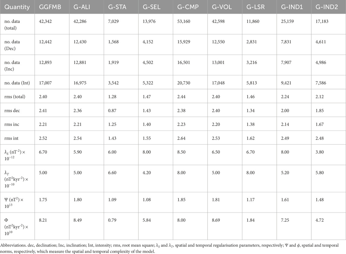
Table 2. Comparison of the nine models based on input data quantity, model misfit to input data, and spatial and temporal regularisation parameters.

The number of input data ranges from just over 7,000 (G-STA) to more than 50, 000 (G-CMP). Except for G-STA, all models have more input data in the interval $\sim$ 800–750 ka, directly around the MB reversal, than before or after (see Table 2; Supplementary Figure S30). The numbers of data for GGFMB, G-ALI, and G-VOL are almost the same. Inputs for G-IND1 are slightly higher than those for G-IND2 over most of the examined period. The numbers of intensity data in G-SEL and G-LSR are comparable, but there are more directional data in G-SEL. The number of intensity data exceeds that for declination or inclination for all models except G-STA and G-SEL.

The trade-off curves used to determine the preferred regularization parameters for the models are displayed in Supplementary Figure S31, indicating the ${\lambda }_S$ and ${\lambda }_T$ that were used to create the models. The temporal variability varies, but the overall spatial complexity is similar among the models (See Table 2). As expected, model G-LSR with only low sedimentation rate data has low resolution, and the resolution for model G-STA with only one stack per region is even lower. Despite the regional data alignment, G-ALI has similar temporal complexity as GGFMB. The highest values is found for G-VOL, while G-CMP with the maximum number of data has a slightly lower value. We assume that the differences in the temporal resolution values among models GGFMB, G-ALI, G-CMP and G-VOL are mainly due to the somewhat subjective choice of regularization parameter. The iterative outlier rejection expectedly removes the largest number of data around 820–760 ka (Supplementary Figure S32), during the MB reversal when the field probably changed more strongly and rapidly than the models can reproduce, and when small errors in dating can have very strong effects in terms of modelling result and deviation of individual data from it, in particular for the directional field components. Interestingly, more directional data were rejected in the late Matuyama (900–800 ka) compared to the early Brunhes (750–700 ka), when most of the models have slightly higher original numbers of data over time on average.

3.2 Fit to data

The normalised rms misfit of the models to the data varied from 1.3 (G-STA) to 2.4 (G-CMP) (Table 2), which is influenced by the amount of input data. Fitting the data to a 1.0 normalised rms misfit should not be expected as age uncertainties are not considered and we do not consider the weights as reliable data uncertainty estimates. The misfits of GGFMB and G-ALI are mostly similar, suggesting that the regional consistency of the paleomagnetic data was not improved by the regional TS alignment process carried out for G-ALI. Similarly, the G-VOL misfit is similar to that of GGFMB, which could be an indication that the small number of volcanic data have little influence on the model despite the higher weighting. The fits of the model G-CMP to inclination and declination data are comparable to those of GGFMB, but the fit to intensity is slightly worse, although G-CMP contains additional data in all components. Histogram distributions of the residuals between the data and model components are displayed in Supplementary Figure S33. They indicate that the intensity misfit has a small positive bias, meaning that model predictions tend to be on average slightly lower than the observed data. The distributions of the declination and inclination residuals are generally symmetric.

As an example of how the models fit the data, we present in Figure 2 the declination, inclination, and intensity model predictions for a high-resolution North-Atlantic sediment record (U1306 (Channell et al., 2014)). This record was selected as the master record for the North Atlantic region because of the high reliability of its age model and its rapid SR of 15 cm/kyr (see Data S1). The comparisons between the model predictions and all original GGFMB input sediment records are displayed in Supplementary Figures S34–S80. In addition to the full time series, enlargements are shown for the period 820–760 ka to provide a more detailed impression of the models’ performances during the reversal. Remember that some models did not include all of the data, or that some of them did so on different age scales (see Supplementary Table S1). In the example in Figure 2, models G-LSR and G-IND2 did not use U1306 as input and we can analyse how well the models fit independent data. Similar assessments of fit to independent data can be conducted on the remaining records (Supplementary Figures S34–S80).

Figure 2

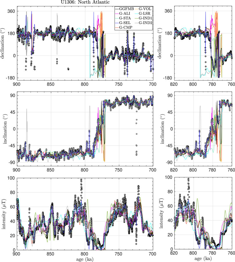
Figure 2. Model predictions for a full-vector paleomagnetic high-resolution record (U1306) (Channell et al., 2014). This record was selected as the master record for North Atlantic region (See Supplementary Material S1). Note that the G-SEL model includes only this record from the North Atlantic, therefore it has the best fit to data. G-LSR and G-IND2 do not include this record. Note that the declination scale spans more than 360° to represent normal variations during both the reverse and normal polarity interval reasonably, which in a few cases leads to apparent disparities when data and model plot 360° offset.

The models provide a reasonable fit as they generally predict most of the paleomagnetic features of the U1306 magnetic field components during the times of stable field (See Figure 2). The amplitudes of fast variations in this record tend to be underestimated, which is not surprising. Millennial scale models in general hardly resolve the full temporal field changes represented by the highest resolution records as similarly good information is not available from all over the world. Extreme declination swings suggested by this record around 887–875 ka and 742 ka are not reproduced by any of the models, and the same is true for the inclination values around 725 ka or the extreme intensity values at 806 ka and 724 ka. However, at least the strong inclination swing is not seen in any of the other Northern Atlantic data so that in some cases also the reliability of the data might be questioned. Rapid and strong regional directional field changes in general can occur when the field is non-dipolar, and in particular fast declination swings can occur when the magnetic pole is close to the location and inclinations are very steep. In a few cases, models predict stronger variations than the data of this record. This effect in general mainly occurs for models that did not include the data and thus may give erroneous interpolations for the location due to influences from surrounding records. The models clearly differ in their representation of the MB reversal in declination and inclination. This is not surprising as the full dynamics of these drastic field changes are not captured by most records and inconsistencies in age scales among records can have strong effects on the models. However, it is noteworthy that all models, including the ones that do not include the record, fit the intensity minimum of U1306 (Figure 2), but all show clear offsets for the intensity minimum around 770–780 ka in records U1308 and U1304 from the same North Atlantic region (Supplementary Figures S35, S37). The high data coverage in this area provides strong constraints for the models regarding the reliable age scales. In the example in Figure 2, the G-SEL model fits the data best since for this model, the record was the only input data for the entire North Atlantic region. Although G-LSR and G-IND2 did not use the record, they properly predict the primary features shown in the data, which adds credibility to the models.

3.3 Dipole evolution

To examine the global evolution of several components of the dipole field as predicted by the nine models, we plot the dipole coefficients (${\mathrm{g}}_1^0$, ${\mathrm{g}}_1^1$, and ${\mathrm{h}}_1^1$), dipole moment (DM), latitude of the geomagnetic pole (dipole latitude DL), dipole power (DP) and non-dipole power (NDP) at core-mantle boundary (CMB) in Figure 3. All models exhibit similar dipole field behaviour over most of the analyzed time period. Only models G-CMP, G-IND1, and G-IND2 differ notably during some intervals.

Figure 3

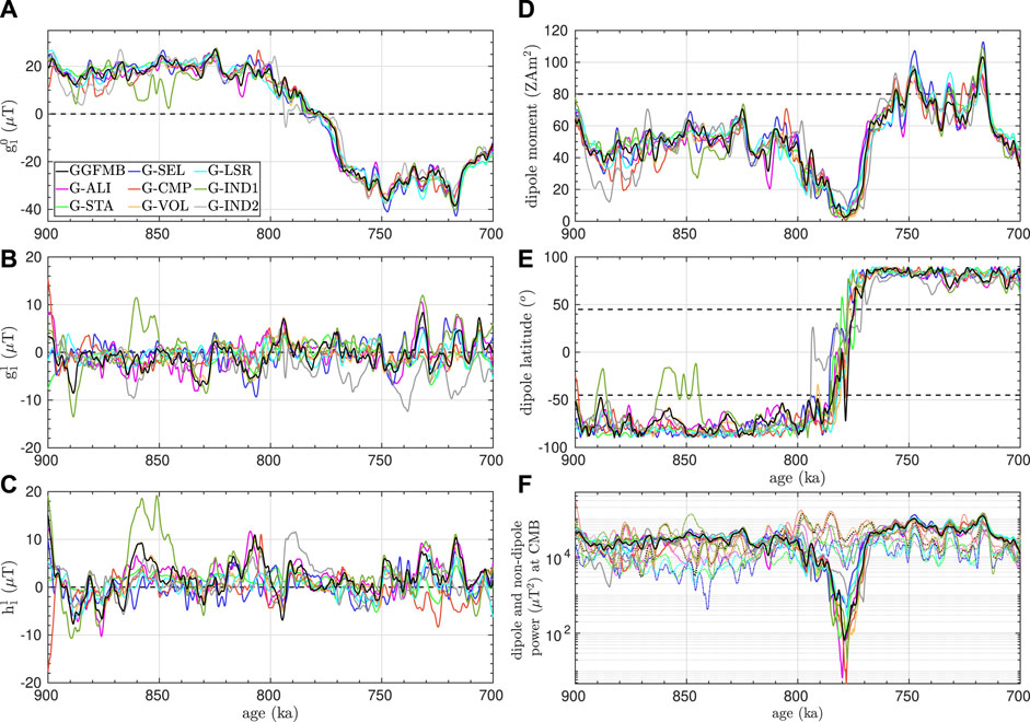
Figure 3. (A–C) Dipole coefficients (${\mathrm{g}}_1^0$, ${\mathrm{g}}_1^1$, and ${\mathrm{h}}_1^1$), (D) dipole moment, (E) latitude of the geomagnetic pole (dipole latitude), and (F) dipole (solid lines) and non-dipole (dashed lines) power of the nine models over the interval 700–900 ka. The approximate value of the 20^th century dipole moment ($\sim$80 ZAm²) is shown by the dashed line in (D). The two dashed lines in (E) represent dipole latitudes of +45° and −45°, within which the magnetic field might be considered to be in a transitional state.

Most of the models agree that the DM oscillated between $\sim$30 and 50 ZAm² from 900 to 800 ka (Figure 3D), never reaching the present-day field value ($\sim$80 ZAm²), while the DL ranged between −90° and −55° (Figure 3E). The dipole tilt was generally low in the late Matuyama, but several models, including the original GGFMB, indicate that occasionally the tilt reached values up to −45°. The field was clearly stronger after the reversal in the Early Brunhes, when all models agree that the DM fluctuated notably between 60 and around 100 ZAm². The dipole tilt also varied less during this time. During the reversal, all models clearly show the previously noted asymmetric slow decay and fast recovery of the DM (Valet and Meynadier, 1993; Meynadier et al., 1994), that has been termed sawtooth behaviour. Almost all agree that the DM dropped to very low values around or below 5 ZAm². G-CMP reaches the lowest DM with 0.1 ZAm², while the DM of G-IND2 did not go below 9 ZAm². Except for G-IND2 (which is constrained by only half of the data set) they also quite consistently give the main polarity change closely around 778 ka, although details in variations of dipole latitude vary. This is not surprising as small differences in the equatorial dipole coefficients can cause clear differences in dipole latitude when the axial dipole contribution is small.

Although the equatorial dipole coefficients differ somewhat among the models, ${\mathrm{h}}_1^1$ appears to have on average slightly larger amplitude variations than ${\mathrm{g}}_1^1$ (Figures 3B, C) in particular during the late Matuyama, potentially indicating preferred dipole tilt directions. None of the models exhibits special behaviour of the equatorial dipole contribution during the reversal. Variations in NDP also differ among the models, but the large scale NDP at the CMB (model resolution $\le$ SH degree 5) is generally lower than the DP during late Matuyama and early Brunhes. While some models predict a rise of NDP with the axial dipole decay during the beginning of the reversal (Figure 3F), others remain at a similar level as before (but G-SEL and G-LSR, to which this applies, have lower NDP than the other models around 870–820 ka). However, all models indicate a brief decrease of NDP during the main polarity change around 780 ka and fluctuated at a somewhat higher level in the early Brunhes than in the late Matuyama. In general, there is a higher degree of model coherence both in dipole and non-dipole evolution after the reversal. This could be indicative of better quality of the younger data with higher consistency among all the records or might reflect that the slightly larger number of data for this time provides improved constraints for the models.

3.4 Global timing and duration of the MB reversal

In order to assess the global timing and duration of the MB reversal we study the globally averaged paleosecular variation index $(P_i)$ and the DP/NDP ratio at the CMB as given by the nine models (Figure 4). The dimensionless $P_i$ index, introduced by Panovska and Constable (2017), evaluates the departure of the virtual geomagnetic pole latitude and virtual dipole moment from the geographic pole and the present-day dipole moment strength, respectively. Field instability phases can be identified by using a threshold of 0.5. Lower values represent a stable field state, whereas values $\ge$0.5 indicate transitional field behaviour. Utilising the DP/NDP ratio with the large scale NDP as resolved by millennia scale paleomagnetic field models, the magnetic field state can be considered stable if the ratio is $\ge$1, and unstable if the ratio is less (Korte et al., 2019).

Figure 4

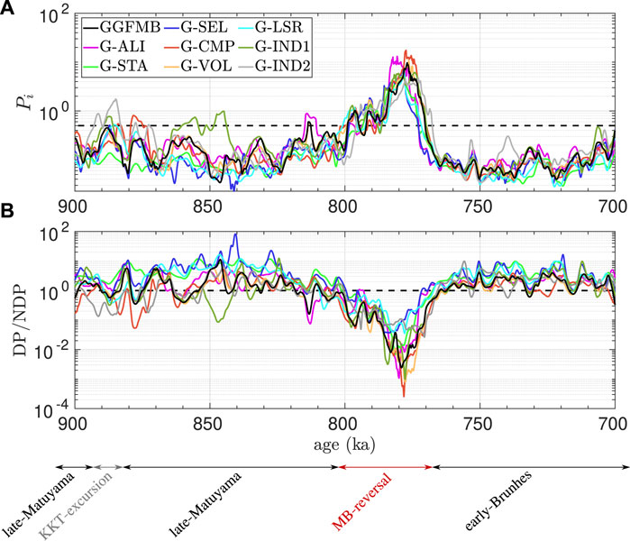
Figure 4. (A) Paleosecular variation index $(P_i)$ and (B) dipole/non-dipole power (DP/NDP) ratio of the nine models over the 700–900 ka interval. The stable field phases of late Matuyama and early Brunhes as well as the MB reversal and the KKT excursion are indicated at the bottom.

The globally averaged $P_i$ curves of the nine models, which were derived from model predictions using an equal area global grid with a distance of 1 × 1° near the equator, are plotted in Figure 4A. The nine curves of DP/NDP are given in Figure 4B. Most of the models generally show $P_i$ values below 0.5 and DP/NDP $\ge$1 during the late Matuyama and early Brunhes, reflecting the stable field states. The early Brunhes appears more stable, while slightly larger $P_i$ values are found in many of the models for the late Matuyama, occasionally exceeding the 0.5 threshold in some models. This is also reflected by the large variability in DP/NDP, but the stronger dispersion of the models impedes a robust interpretation for this time interval. The known KKT excursion around 880 ka is reflected by a $P_i$ peak or DP/NDP minimum of various amplitudes in most of the models, while only some of the models suggest that there might have been additional times of transitional field occurrence before the onset of the MB reversal.

The sawtooth asymmetry of the DM evolution during the reversal is also clearly seen in both $P_i$ and DP/NDP. The start, mid-point, end, and duration of the reversal process constrained by $P_i$ and DP/NDP are calculated for the nine models and listed in Supplementary Table S2. Using the first and last occurrence of $P_i\ge 0.5$ (Figure 4A) as a criteria, our models indicate that the surface geomagnetic field reversal began 802–796 ka and terminated at 773–768 ka. The reversal process globally spanned around 21 to 32 ka, with the shortest duration seen in G-STA and the largest duration observed in G-CMP. More data and a wider regional coverage tend to give longer durations, which might reflect the complexity of the reversal process, although we cannot fully rule out that inconsistencies in age models of the records bias the results. The highest $P_i$ values are found almost simultaneously in all of the models at around 778–777 ka (Figure 4), which corresponds to the time of the major drops in DM and DP (See Figure 3) and the main global polarity change, i.e., the main phase of the reversal. The DP/NDP ratio increased briefly during this period since the NDP also had a small minimum (See Figure 3F). Models G-ALI and G-STA, based on regionally aligned and stacked data, respectively, suggest a slightly earlier occurrence than the models using more individual data.

The occurrence of a precursor phase of transitional field prior to the main reversal has been found in several sediment records (e.g., Hartl and Tauxe, 1996; Valet et al., 2014; Singer et al., 2019). All of our models indicate the existence of one or more precursors ($P_i$ exceeding 0.5 but dropping below again before the main reversal phase). We cannot rule out that one event might be erroneously interpreted as two or more events by a global model if the age scales of various records are inconsistent. However, a likely explanation is that during the slow decay of the axial dipole, some variations lead to regionally occurring and disappearing transitional field, especially in a phase when the DM was low. This would appear as a number of regionally different precursors.

3.5 Global morphology of the Matuyama-Brunhes reversal

The evolution of the global field is investigated here in terms of surface field intensity and radial field $(B_r)$ at the CMB. Using Supplementary Movies S1–S9, the evolution of the field morphology of the entire reversal (and across the full 700–900 ka interval) can be studied in detail. In Figure 5 we display snapshots at the beginning (global $P_i$ first reaching 0.5), middle (maximum global $P_i$) and end (last occurrence of global $P_i\ge 0.5$). Given that the reversal is not observed fully concurrently in all models (Figure 4), the displayed times vary.

Figure 5

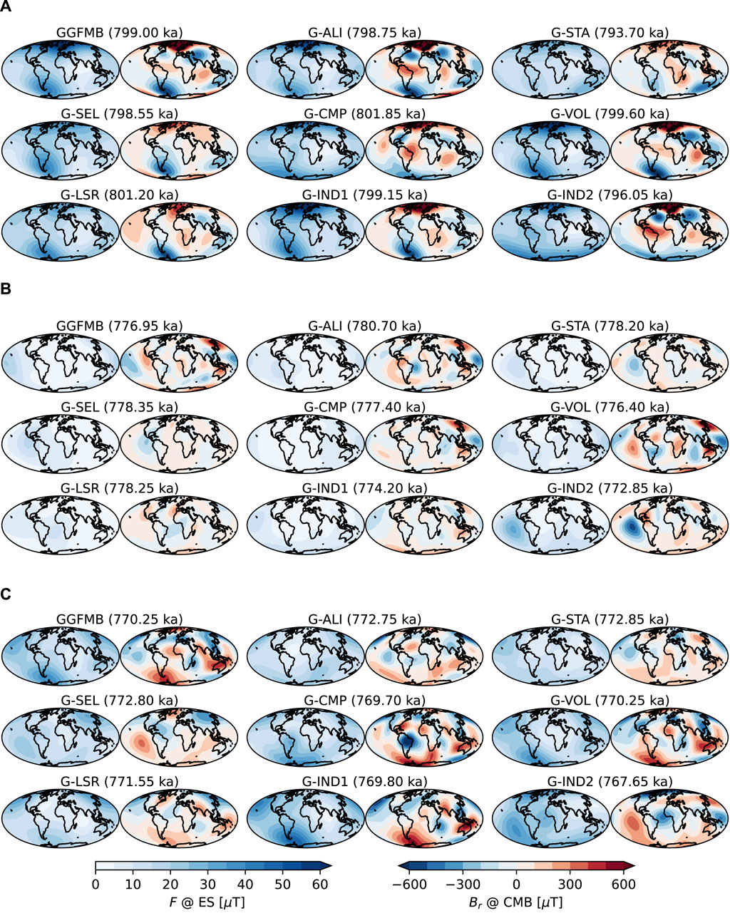
Figure 5. Field morphology at: (A) begin, (B) middle, and (C) end of the Matuyama-Brunhes reversal, according to the nine global models. For each model snapshots of (left) surface field intensity (F) and (right) radial field component $(B_r)$ at the core-mantle boundary (CMB) are given for specific times representing the respective phase of the reversal in each model.

The models clearly differ in many details and the field morphology, in particular at the CMB, should be interpreted with caution. However, in the early phase of the reversal nearly all models, including the two fully independent ones (G-IND1 and G-IND2), indicate the development of two reverse flux patches (with respect to the stable inverse field of the late Matuyama) over Asia and the Atlantic Ocean, and in many cases reverse flux in high southern latitudes (Figure 5A). The southern hemisphere reverse flux reaches into the tangent cylinder early in the process, while the northern hemisphere reverse flux manifests just outside and only enters the tangent cylinder towards the main phase of the reversal. Reverse CMB flux implies weak surface field intensity in the same areas. None of the models shows weak intensity over the region of the present-day South Atlantic Anomaly (SAA). This supports the findings that the SAA should not be seen as an indication for an upcoming reversal or excursion. This had been suggested by Pavón-Carrasco and De Santis (2016), but already found not to be the case for the Laschamps excursion (at 41 ka) (Brown et al., 2018) and further excursions during the past 100 kyr (Panovska et al., 2019).

Related to the observed occurrence of precursors in the further evolution of the reversal, the magnetic field underwent some variations in stability during which the initially observed reverse flux patches became weaker again or disappeared completely. This continued to the middle phase of the reversal (Figure 5B), when the dipole moment reached its minimum (in some cases close to zero) (see Figure 3). In general, these non-dipole field variations are not resolved robustly and appear differently in the various models, as is also the case for the snapshots in Figure 5B. Surface field intensity was clearly very low all over the globe at this time.

Given that our analyses above indicated a higher coherence of the different models after than before the reversal, it is surprising that Figure 5C still gives a very incoherent picture of the CMB field morphology at the end of the reversal, when the axial dipole contribution and surface field intensity gain strength. However, one aspect that appears rather consistent in most models is that reverse flux (now related to the Brunhes normal field direction) occurs longer in the northern than southern hemisphere before the field gets strongly dipole dominated.

3.6 Time-averaged field

The time averaged radial field configuration at the CMB during the interval 700–900 ka for the two stable field intervals of late Matuyama (900–800 ka) and early Brunhes (770–700 ka) and the MB reversal (800–770 ka) is shown in Figures 6A–C) and also compared to the time-averaged $B_r$ over the past 100 kyr (GGF100k; Panovska et al. (2018)) and 10 kyr (CALS10k.2; Constable et al. (2016)) shown in Figure 6D. For compatibility, these models were also evaluated to spherical harmonic degree 6.

Figure 6

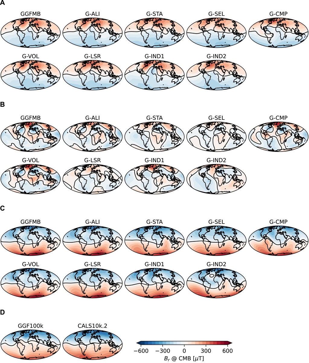
Figure 6. Time-averaged radial field $(B_r)$ at the core-mantle boundary for the nine models, for late Matuyama (A), the MB reversal (B) and the early Brunhes (C). Panel (D) shows the 100–0 kyr and 10–0 kyr-averaged $B_r$ maps of models GGF100k (Panovska et al., 2018) and CALS10k.2 (Constable et al., 2016), respectively.

The time averages again clearly reflect a stronger field during the early Brunhes than the late Matuyama. Although the averages of the different models vary in details, for the stable periods they show a similar structure in general. This includes a tendency for two mid-latitude intense flux lobes in the northern hemisphere in the late Matuyama (Figure 6A), similar to the 10 kyr average (Figure 6D). The southern hemisphere field seems to have been weaker than the northern during this time. Southern hemisphere structure seems slightly less complex both in late Matuyama and early Brunhes. This might be due to the limited southern hemisphere data coverage. However, the fact that all models, including the ones from reduced and extended data sets, indicate the asymmetry in strength, supports the hypothesis that this is a real magnetic field characteristic. For the early Brunhes, the northern hemisphere flux distribution varies notably among the models, similar to our finding for clear differences in field morphology at the ending phase of the reversal. For example, GGFMB, G-ALI and G-VOL suggest weak flux in the north western Atlantic and G-IND2 even has a small reverse flux patch in the northern Atlantic. On the other hand, G-CMP, which is constrained by additional records, suggests strong normal flux in this region, and G-STA and G-SEL (based on less records, stacked and selected, respectively) indicate more uniform flux from north America to Europe (Figure 6C).

During the reversal (Figure 6B), most of the models, including the two fully independent ones (G-IND1 and G-IND2) indicate two flux lobes in very similar places as the intense flux lobes observed during the late Matuyama, but with opposite sign (i.e., reverse compared to the Matuyama polarity). It seems that also during this interval there is on average less structure and weaker flux in the southern than the northern hemisphere.

4 Conclusion

Based on a combination of published paleomagnetic sediment records and volcanic data, we have developed a suite of eight new global paleomagnetic field models spanning 700 to 900 ka, including the Matuyama-Brunhes reversal and the Kamikatsura excursion. They were derived from modifications of the input data used to construct the GGFMB (global geomagnetic field model for the Matuyama-Brunhes reversal) model in order to explore the influence of subjective data choices and study the robustness of geomagnetic field characteristics found from this model.

The utilised modelling technique impedes a quantitative evaluation of the similarities and differences across the models. We assume that the coherence or disparity of the range of models gives a reasonable indication of the reliability of certain magnetic field features. Thus, it was feasible to distinguish between robust and non-robust magnetic field characteristics during the MB reversal by associating the model output with the relevant data set selection. Accordingly, the following characteristics seem robustly resolved: All models confirm a sawtooth pattern of slow dipole moment decay and fast recovery with a drop to values around or below 5 ZAm². A precursory period of transitional field states occurred during the decay and prior to the main global reversal. The decay and recovery of the axial dipole contribution is the main driver of the reversal, the equatorial dipole and non-dipole contributions do not play a strong role. The non-dipole power seems to increase slightly during the early phases of dipole decay, but drops during the main phase of the reversal. All models suggest a significantly lower dipole moment before the reversal in the late Matuyama than in the early Brunhes. The global duration of the event lies between 21 (G-STA) and 32 kyr (G-CMP), with all models agreeing that the main global polarity change occurred around 778 ka. The duration might be overestimated with the addition of records if age-depth models are not compatible, while the duration might be underestimated by alignment of records based on the magnetic field signal. Due to the non-dipole dominance during the reversal, the regional occurrence of the main directional field change and also the regional duration of the whole reversal process vary. The field morphology around the onset of the reversal seems to be generally robustly resolved and does not resemble the present day South Atlantic Anomaly structure. Instead, two reverse flux patches occur in the northern hemisphere at that time. Better coherence of time series of global field properties like DM, DP/NDP or $P_i$ index for the early Brunhes than the late Matuyama suggests that the data are more consistent and the models should resolve field characteristics better after the reversal. The Kamikatsura excursion was in general robustly identified around 890–884 ka.

However, other field properties, including the following, should be interpreted with caution. Details of field predictions, in particular in regions where few or no data exist, and especially the rapid directional changes during the reversal, might not be reliably resolved by individual models. Similarly, details of the field morphology, in particular at the CMB during the time when the axial dipole is weak and small-scale structures dominate are not robustly resolved and should not be interpreted. This also applies to the number and regions of occurrence of the transitional field precursors, and (regional) excursions occurring in some of the models in the late Matuyama in addition to the Kamikatsura excursion. These features can only be better constrained in the models when additional data become available.

In general, the global reconstruction of the MB reversal would benefit strongly from more data originating in the southern hemisphere, which so far is sparsely covered. GGFMB seems a reasonable model for many applications given the currently existing data that have recorded the event. To get an idea of the reliability of certain magnetic field characteristics predicted by the model it is advisable to compare the results from different reconstructions.

Data availability statement

The datasets presented in this study can be found in online repositories. The names of the repository/repositories and accession number(s) can be found below: The models can be found at https://earthref.org/ERDA/2739/. Models animation (Supplementary Movies S1–S9) are available at https://earthref.org/ERDA/2736/.

Author contributions

ANM: Data curation, Formal Analysis, Investigation, Methodology, Software, Visualization, Writing–original draft. MK: Conceptualization, Funding acquisition, Investigation, Methodology, Project administration, Resources, Supervision, Validation, Writing–review and editing. SP: Data curation, Formal Analysis, Investigation, Methodology, Software, Writing–review and editing. MS: Conceptualization, Methodology, Software, Validation, Visualization, Writing–review and editing.

Funding

The author(s) declare that financial support was received for the research, authorship, and/or publication of this article. ANM was supported by the Alexander von Humboldt Foundation. ANM and MK acknowledge funding by the Deutsche Forschungsgemeinschaft (DFG, German Research Foundation) - project number 521251212. SP acknowledges funding by the DFG - project number 521548146, and MS acknowledges funding by the DFG - project number 388291411.

Conflict of interest

The authors declare that the research was conducted in the absence of any commercial or financial relationships that could be construed as a potential conflict of interest.

Publisher’s note

All claims expressed in this article are solely those of the authors and do not necessarily represent those of their affiliated organizations, or those of the publisher, the editors and the reviewers. Any product that may be evaluated in this article, or claim that may be made by its manufacturer, is not guaranteed or endorsed by the publisher.

Supplementary material

The Supplementary Material for this article can be found online at: https://www.frontiersin.org/articles/10.3389/feart.2024.1443095/full#supplementary-material

References

Balbas, A. M., Koppers, A. A., Clark, P. U., Coe, R. S., Reilly, B. T., Stoner, J. S., et al. (2018). Millennial-Scale instability in the geomagnetic field prior to the Matuyama-Brunhes reversal. Geochem. Geophys. Geosystems 19, 952–967. doi:10.1002/2017gc007404

CrossRef Full Text | Google Scholar

Brown, M. C., Korte, M., Holme, R., Wardinski, I., and Gunnarson, S. (2018). Earth’s magnetic field is probably not reversing. Proc. Natl. Acad. Sci. 115, 5111–5116. doi:10.1073/pnas.1722110115

PubMed Abstract | CrossRef Full Text | Google Scholar

Cande, S. C., and Kent, D. V. (1995). Revised calibration of the geomagnetic polarity timescale for the Late Cretaceous and Cenozoic. J. Geophys. Res. Solid Earth 100, 6093–6095. doi:10.1029/94jb03098

CrossRef Full Text | Google Scholar

Channell, J. E. T. (2017). Complexity in matuyama–brunhes polarity transitions from north Atlantic IODP/ODP deep-sea sites. Earth Planet. Sci. Lett. 467, 43–56. doi:10.1016/j.epsl.2017.03.019

CrossRef Full Text | Google Scholar

Channell, J. E. T., Curtis, J. H., and Flower, B. P. (2004). The Matuyama-Brunhes boundary interval (500-900 ka) in North Atlantic drift sediments. Geophys. J. Int. 158, 489–505. doi:10.1111/j.1365-246x.2004.02329.x

CrossRef Full Text | Google Scholar

Channell, J. E. T., Singer, B. S., and Jicha, B. R. (2020). Timing of Quaternary geomagnetic reversals and excursions in volcanic and sedimentary archives. Quat. Sci. Rev. 228, 106114. doi:10.1016/j.quascirev.2019.106114

CrossRef Full Text | Google Scholar

Channell, J. E. T., Wright, J. D., Mazaud, A., and Stoner, J. S. (2014). Age through tandem correlation of Quaternary relative paleointensity (RPI) and oxygen isotope data at IODP Site U1306 (Eirik Drift, SW Greenland). Quat. Sci. Rev. 88, 135–146. doi:10.1016/j.quascirev.2014.01.022

CrossRef Full Text | Google Scholar

Constable, C., Korte, M., and Panovska, S. (2016). Persistent high paleosecular variation activity in southern hemisphere for at least 10 000 years. Earth Planet. Sci. Lett. 453, 78–86. doi:10.1016/j.epsl.2016.08.015

CrossRef Full Text | Google Scholar

Creer, K., Tucholka, P., and Barton, C. (1983). Geomagnetism of baked clays and recent sediments. Amsterdam ; New York: Elsevier.

Google Scholar

Dinarès-Turell, J., Sagnotti, L., and Roberts, A. P. (2002). Relative geomagnetic paleointensity from the Jaramillo Subchron to the Matuyama/Brunhes boundary as recorded in a Mediterranean piston core. Earth Planet. Sci. Lett. 194, 327–341. doi:10.1016/s0012-821x(01)00563-5

CrossRef Full Text | Google Scholar

Elsasser, W., Ney, E., and Winckler, J. (1956). Cosmic-ray intensity and geomagnetism. Nature 178, 1226–1227. doi:10.1038/1781226a0

CrossRef Full Text | Google Scholar

Gubbins, D. (1983). Geomagnetic field analysis—I. Stochastic inversion. Geophys. J. Int. 73, 641–652. doi:10.1111/j.1365-246x.1983.tb03336.x

CrossRef Full Text | Google Scholar

Gubbins, D. (2004). Time series analysis and inverse theory for geophysicists. Cambridge: Cambridge University Press.

Google Scholar

Hartl, P., and Tauxe, L. (1996). A precursor to the Matuyama/Brunhes transition-field instability as recorded in pelagic sediments. Earth Planet. Sci. Lett. 138, 121–135. doi:10.1016/0012-821x(95)00231-z

CrossRef Full Text | Google Scholar

Ingham, M., and Turner, G. (2008). Behaviour of the geomagnetic field during the Matuyama–Brunhes polarity transition. Phys. Earth Planet. Interiors 168, 163–178. doi:10.1016/j.pepi.2008.06.008

CrossRef Full Text | Google Scholar

Korte, M., Brown, M. C., Panovska, S., and Wardinski, I. (2019). Robust characteristics of the Laschamp and Mono Lake geomagnetic excursions: results from global field models. Front. Earth Sci. 7, 86. doi:10.3389/feart.2019.00086

CrossRef Full Text | Google Scholar

Korte, M., Donadini, F., and Constable, C. (2009). Geomagnetic field for 0–3 ka: 2. A new series of time-varying global models. Geochem. Geophys. Geosystems 10. doi:10.1029/2008gc002297

CrossRef Full Text | Google Scholar

Leonhardt, R., and Fabian, K. (2007). Paleomagnetic reconstruction of the global geomagnetic field evolution during the Matuyama/Brunhes transition: iterative Bayesian inversion and independent verification. Earth Planet. Sci. Lett. 253, 172–195. doi:10.1016/j.epsl.2006.10.025

CrossRef Full Text | Google Scholar

Love, J., and Mazaud, A. (1997). A database for the Matuyama-Brunhes magnetic reversal. Phys. earth Planet. interiors 103, 207–245. doi:10.1016/s0031-9201(97)00034-4

CrossRef Full Text | Google Scholar

Lund, S. P., and Keigwin, L. (1994). Measurement of the degree of smoothing in sediment paleomagnetic secular variation records: an example from late Quaternary deep-sea sediments of the Bermuda Rise, western North Atlantic Ocean. Earth Planet. Sci. Lett. 122, 317–330. doi:10.1016/0012-821x(94)90005-1

CrossRef Full Text | Google Scholar

Mahgoub, A. N., Korte, M., and Panovska, S. (2023a). Characteristics of the matuyama-brunhes magnetic field reversal based on a global data compilation. J. Geophys. Res. Solid Earth 128, e2022JB025286. doi:10.1029/2022jb025286

CrossRef Full Text | Google Scholar

Mahgoub, A. N., Korte, M., and Panovska, S. (2023b). Global geomagnetic field evolution from 900 to 700 ka including the matuyama-brunhes reversal. J. Geophys. Res. Solid Earth 128, e2023JB026593. doi:10.1029/2023jb026593

CrossRef Full Text | Google Scholar

Meynadier, L., Valet, J.-P., Bassinot, F. C., Shackleton, N. J., and Guyodo, Y. (1994). Asymmetrical saw-tooth pattern of the geomagnetic field intensity from equatorial sediments in the Pacific and Indian Oceans. Earth Planet. Sci. Lett. 126, 109–127. doi:10.1016/0012-821x(94)90245-3

CrossRef Full Text | Google Scholar

Nagy, E. A., and Valet, J.-P. (1993). New advances for paleomagnetic studies of sediment cores using u-channels. Geophys. Res. Lett. 20, 671–674. doi:10.1029/93gl00213

CrossRef Full Text | Google Scholar

Noel, M., and Batt, C. (1990). A method for correcting geographically separated remanence directions for the purpose of archaeomagnetic dating. Geophys. J. Int. 102, 753–756. doi:10.1111/j.1365-246x.1990.tb04594.x

CrossRef Full Text | Google Scholar

Ogg, J. (2020). “Geomagnetic polarity time scale,” in Geologic time scale 2020 (Elsevier), 159–192.

CrossRef Full Text | Google Scholar

Panovska, S., and Constable, C. (2017). An activity index for geomagnetic paleosecular variation, excursions, and reversals. Geochem. Geophys. Geosystems 18, 1366–1375. doi:10.1002/2016gc006668

CrossRef Full Text | Google Scholar

Panovska, S., Constable, C., and Korte, M. (2018). Extending global continuous geomagnetic field reconstructions on timescales beyond human civilization. Geochem. Geophys. Geosystems 19, 4757–4772. doi:10.1029/2018gc007966

CrossRef Full Text | Google Scholar

Panovska, S., Korte, M., and Constable, C. G. (2019). One hundred thousand years of geomagnetic field evolution. Rev. Geophys. 57, 1289–1337. doi:10.1029/2019rg000656

CrossRef Full Text | Google Scholar

Pavón-Carrasco, F. J., and De Santis, A. (2016). The South Atlantic Anomaly: the key for a possible geomagnetic reversal. Front. Earth Sci. 4. doi:10.3389/feart.2016.00040

CrossRef Full Text | Google Scholar

Roberts, A. P. (2006). High-resolution magnetic analysis of sediment cores: strengths, limitations and strategies for maximizing the value of long-core magnetic data. Phys. Earth Planet. Interiors 156, 162–178. doi:10.1016/j.pepi.2005.03.021

CrossRef Full Text | Google Scholar

Roberts, A. P. (2015). Magnetic mineral diagenesis. Earth-Science Rev. 151, 1–47. doi:10.1016/j.earscirev.2015.09.010

CrossRef Full Text | Google Scholar

Roberts, A. P., and Winklhofer, M. (2004). Why are geomagnetic excursions not always recorded in sediments? Constraints from post-depositional remanent magnetization lock-in modelling. Earth Planet. Sci. Lett. 227, 345–359. doi:10.1016/j.epsl.2004.07.040

CrossRef Full Text | Google Scholar

Sagnotti, L. (2018). New insights on sediment magnetic remanence acquisition point out complexity of magnetic mineral diagenesis. Geology 46, 383–384. doi:10.1130/focus042018.1

CrossRef Full Text | Google Scholar

Sagnotti, L., Budillon, F., Dinarès-Turell, J., Iorio, M., and Macrì, P. (2005). Evidence for a variable paleomagnetic lock-in depth in the Holocene sequence from the Salerno Gulf (Italy): implications for “high-resolution” paleomagnetic dating. Geochem. Geophys. Geosystems 6. doi:10.1029/2005gc001043

CrossRef Full Text | Google Scholar

Sagnotti, L., Giaccio, B., Liddicoat, J. C., Nomade, S., Renne, P. R., Scardia, G., et al. (2016). How fast was the Matuyama–Brunhes geomagnetic reversal? A new subcentennial record from the Sulmona Basin, central Italy. Geophys. J. Int. 204, 798–812. doi:10.1093/gji/ggv486

CrossRef Full Text | Google Scholar

Sagnotti, L., Scardia, G., Giaccio, B., Liddicoat, J. C., Nomade, S., Renne, P. R., et al. (2014). Extremely rapid directional change during Matuyama-Brunhes geomagnetic polarity reversal. Geophys. J. Int. 199, 1110–1124. doi:10.1093/gji/ggu287

CrossRef Full Text | Google Scholar

Shao, J.-C., Fuller, M., Tanimoto, T., Dunn, J., and Stone, D. (1999). Spherical harmonic analyses of paleomagnetic data: the time-averaged geomagnetic field for the past 5 Myr and the Brunhes-Matuyama reversal. J. Geophys. Res. Solid Earth 104, 5015–5030. doi:10.1029/98jb01354

CrossRef Full Text | Google Scholar

Simon, Q., Suganuma, Y., Okada, M., Haneda, Y., and Team, A. (2019). High-resolution 10Be and paleomagnetic recording of the last polarity reversal in the Chiba composite section: age and dynamics of the Matuyama–Brunhes transition. Earth Planet. Sci. Lett. 519, 92–100. doi:10.1016/j.epsl.2019.05.004

CrossRef Full Text | Google Scholar

Singer, B. S., Jicha, B. R., Mochizuki, N., and Coe, R. S. (2019). Synchronizing volcanic, sedimentary, and ice core records of Earth’s last magnetic polarity reversal. Sci. Adv. 5, eaaw4621. doi:10.1126/sciadv.aaw4621

PubMed Abstract | CrossRef Full Text | Google Scholar

Suttie, N., and Nilsson, A. (2019). Archaeomagnetic data: the propagation of an error. Phys. Earth Planet. Interiors 289, 73–74. doi:10.1016/j.pepi.2019.02.008

CrossRef Full Text | Google Scholar

Valet, J.-P., Bassinot, F., Bouilloux, A., Bourlès, D., Nomade, S., Guillou, V., et al. (2014). Geomagnetic, cosmogenic and climatic changes across the last geomagnetic reversal from Equatorial Indian Ocean sediments. Earth Planet. Sci. Lett. 397, 67–79. doi:10.1016/j.epsl.2014.03.053

CrossRef Full Text | Google Scholar

Valet, J.-P., and Fournier, A. (2016). Deciphering records of geomagnetic reversals. Rev. Geophys. 54, 410–446. doi:10.1002/2015rg000506

PubMed Abstract | CrossRef Full Text | Google Scholar

Valet, J.-P., and Meynadier, L. (1993). Geomagnetic field intensity and reversals during the past four million years. Nature 366, 234–238. doi:10.1038/366234a0

CrossRef Full Text | Google Scholar

Van Zijl, J., Graham, K., and Hales, A. (1962). The palaeomagnetism of the Stormberg Lavas, II. The behaviour of the magnetic field during a reversal. Geophys. J. R. Astronomical Soc. 7, 169–182. doi:10.1111/j.1365-246x.1962.tb00366.x

CrossRef Full Text | Google Scholar

Whaler, K., and Gubbins, D. (1981). Spherical harmonic analysis of the geomagnetic field: an example of a linear inverse problem. Geophys. J. Int. 65, 645–693. doi:10.1111/j.1365-246x.1981.tb04877.x

CrossRef Full Text | Google Scholar