Enhancing slope stability prediction through integrated PCA-SSA-SVM modeling: a case study of LongLian expressway

China is one of the regions most frequently affected by landslides, which have significant socio-economic impacts. Traditional slope stability analysis methods, such as the limit equilibrium method, limit analysis method, and finite element method, often face limitations due to computational complexity and the need for extensive soil property data. This study proposes a novel approach that combines Principal Component Analysis (PCA), Sparrow Search Algorithm (SSA), and Support Vector Machine (SVM) to improve the accuracy of slope stability prediction. PCA effectively reduces data dimensionality while retaining critical information. SSA optimizes SVM parameters, addressing the limitations of traditional optimization methods. The integrated PCA-SSA-SVM model was applied to a dataset of 257 slope stability samples and validated using five-fold cross-validation to ensure the model’s generalization capability. The results show that the model exhibits superior performance in prediction accuracy, precision, recall, and F1-score, with the test set achieving an accuracy of 84.6%, a recall of 84.7%, a precision of 83.1%, and an F1-score of 84.6%. The model’s robustness was further validated using slope data from the LongLian Expressway, demonstrating high consistency with the actual stability status. These findings indicate that the PCA-SSA-SVM-based slope stability prediction model has significant potential for practical engineering applications, providing a reliable and efficient tool for slope stability forecasting. Classify the training samples through cross-validation, using the accuracy of cross-validation as the fitness of the sparrow individual. Retain the optimal fitness value and position information.

1 Introduction

China is notably one of the regions in Asia, if not the world, that frequently witnesses landslide disasters. According to credible sources (Li et al., 2022; Moayedi et al., 2019; Wei et al., 2021; Xie et al., 2021), between 2011 and 2020, the country experienced over 100,000 geological disasters, of which a staggering 70,000 were landslides, leading to more than 5,000 casualties. The economic impact was profound, resulting in direct losses amounting to 45 billion yuan (Hu et al., 2021). Considering the annual number of geological disasters, it’s alarming to note that landslides consistently constitute over half of these incidents. These landslides, predominantly resulting from slope instability, unleash a multitude of repercussions. They not only cause severe property damage but also result in casualties, traffic disruptions, destruction of homes, hindrances in daily life, and considerable production losses.

To illustrate the scale and implications of such events, let’s consider a significant landslide incident from 2019 in Shuicheng County, Liupanshui City, Guizhou Province. This colossal landslide was triggered primarily due to rainfall infiltration causing slope instability. The aftermath was devastating: the surrounding houses crumbled, resulting in numerous casualties. The direct economic ramifications of this single event reached CNY 190 million, with the volume of displaced land estimated to be around 1.8 million m³.

Therefore, accurate analysis and evaluation of slope stability hold significant practical importance. Through effective analysis, treatment, and protection of slopes, casualties and economic losses can be prevented or reduced. Currently, the primary methods used both domestically and internationally include the limit equilibrium method, the limit analysis method, and the finite element method. The limit equilibrium method is one of the first applied to slope stability analysis due to its clear concept and straightforward calculations. Duncan (1996) further analyzed and discussed the influence of different simplified methods and assumptions on the limit equilibrium analysis results of slopes. However, due to its various assumptions, this method has evolved into several different classification methods, typically divided into strict and non-strict segmentation methods. The basic idea of the limit analysis method to solve the slope stability coefficient is to first divide the assumed slip surface into oblique strips, then establish a coordinated velocity field based on the deformation coordination basis, and finally calculate according to the principle that internal energy dissipation equals the external force. Sloan (1989) improved and optimized the lower bound principle finite element method combined with a mathematical programming method to find the lower bound solution of the slope stability safety factor. Although the limit analysis method is widely used in geotechnical engineering, it is challenging to analyze complex shapes and heterogeneous geotechnical engineering cases. Moreover, due to the subjective assumptions made by the limit analysis method, its further application has been significantly limited. As one of the most widely used numerical analysis methods, the finite element method has developed into two main research directions: the finite element strength reduction method and the finite element limit equilibrium method. Zienkiewicz et al. (1975) proposed an alternative analytical approach that eliminates the necessity of presupposing the configuration of the sliding surface. Central to this methodology is the systematic reduction of strength parameters, namely cohesion (c) and internal friction angle (φ). The decrement value of these parameters at the critical juncture is designated as the stability coefficient for the geomaterial mass.

Stability coefficient is one of the important indexes to evaluate whether the slope is unstable. The stability coefficient values obtained by using different slope stability analysis methods under different working conditions need to be systematically verified (Wang et al., 2022; Zhang W. et al., 2022). For different types and different conditions of slopes, it is necessary to judge the practicability of these methods. However, it is often computationally intensive, requires specialized software and highperformance computer hardware, and requires detailed soil property data (Zhang et al., 2023). Recently, machine learning has found efficacious applications across various civil engineering challenges, notably in slope stability evaluation. The stability of mine slopes is influenced by a myriad of factors that exhibit substantial intercorrelation, necessitating heightened precision in predictive modeling (Xu et al., 2013; Suman et al., 2016; Luan et al., 2023; Lu and Rosenbaum, 2003).Combined with the artificial intelligence algorithm that has emerged in recent years, experts and scholars at home and abroad have proposed many practical models for slope stability prediction research, and have achieved good results. By training a large amount of data, machine learning models can capture the complex relationship between soil and slope characteristics without the need for a clear physical or empirical model. For example, Gu et al. (2009) employed the PCA-GEP algorithm for slope stability prediction and analysis, obtaining favorable outcomes. Chen et al. (2014) utilized PCA in tandem with the BP neural network to anticipate varying types of slope stability, resulting in satisfactory model outcomes. Meanwhile, Bu et al. (2009) introduced a realcoded DE-BP neural network predictive model leveraging the differential evolution algorithm (DE), achieving noteworthy predictive precision. BP neural network models, despite their widespread application in pattern recognition and predictive modeling, exhibit some clear limitations. The primary issue is their propensity to get trapped in local minima, potentially leading to suboptimal model performance. Additionally, BP networks often struggle with overfitting, particularly when dealing with small datasets or a large number of features. They also require significant training time and resources, especially when the network architecture is deep. In the face of these limitations, Support Vector Machine (SVM) models demonstrate their strengths. SVMs enhance classification efficiency by maximizing the margin of the decision boundary, making them more effective in dealing with nonlinear problems and demonstrating superior generalization capabilities when predicting unknown data. The kernel trick in SVMs enables them to efficiently handle highdimensional data, and they are generally less prone to overfitting, which is particularly valuable for complex pattern recognition challenges. Zhang et al. (Bu et al., 2009), aiming for rapid evaluation of the stability of redbed highway slopes, established a model centered around the SVM algorithm for quick assessment of such slopes, applying it to 16 slopes along the Renmu-Xin Expressway. However, the performance of the SVM model can significantly diminish without proper data preprocessing. Jin et al. (Zhang S. et al., 2022), on the other hand, employed the Sparrow Search Algorithm (SSA) to optimize the Support Vector Machine (SVM), creating an SSA-SVM model for intelligent prediction of slope instability, demonstrating notable advantages in forecasting such events. Ding et al. (Jin et al., 2022) proposed a slope stability prediction model based on Principal Component Analysis (PCA) and Support Vector Machine (SVM), where PCA was used to extract principal components as inputs for SVM training. The results indicated that this method could reduce the dimensionality of input variables and enhance the precision of slope stability prediction in engineering. However, previous studies, while effective, often faced challenges with high-dimensional datasets and computational demands. Conventional models struggled with multicollinearity among input variables, leading to less accurate predictions and increased computational complexity. Our study introduces an innovative approach that leverages the strengths of three robust techniques: Principal Component Analysis (PCA), the Sparrow Search Algorithm (SSA), and Support Vector Machines (SVM). PCA effectively reduces the number of features in a dataset while retaining crucial information, simplifying subsequent model training and computational demands. SSA, an emerging optimization technique known for its strong global search capabilities and fast convergence, optimizes the parameters of the SVM, addressing limitations of traditional optimization methods used in previous studies. SVM excels in classification and regression tasks, providing superior generalization capabilities compared to other machine learning models. By combining these three approaches, the PCA-SSA-SVM model can effectively process high-dimensional data, improve prediction accuracy through optimal parameter selection, and achieve high-precision predictions. This integrated method is particularly suited for complex data processing tasks that require feature dimensionality reduction, model parameter optimization, and high-precision predictions. Our study introduces a novel hybrid model for slope stability prediction, addressing limitations of previous models. By reducing dimensionality and optimizing model parameters simultaneously, our approach enhances predictive performance and computational efficiency. The application of this model to real-world engineering data, such as the LongLian Expressway slopes, demonstrates its practical utility and effectiveness, achieving a high degree of accuracy and reliability in predictions. In this research, parameters such as rock weight (γ), cohesion (C), internal friction angle (φ), slope height (H), slope angle (β), and pore water pressure (γu) are designated as input variables, with the slope safety factor serving as the output variable. PCA is used to reduce the dimensionality of these input variables, selecting fewer and linearly independent factors for data prediction. The SSA-SVM model then trains these new input variables. This methodology presents an innovative avenue for slope stability forecasting, addressing limitations of previous studies and providing a robust, accurate predictive model.

2 Method

2.1 Principal component analysis

Principal Component Analysis (PCA) is a statistical method used to simplify the dimension of the data set while retaining as much variability as possible in the original data. It is widely used in data compression, feature extraction and data visualization.

Step.1 Centralize the data (reduce the mean value of each dimension to 0), as shown in Equation 1.

$z_{ij}=\frac{x_{ij}-{\overline{x}}_j}{{\sigma }_{x_j}}(1)$

where ${\overline{x}}_j$ is the arithmetic mean of $x_{ij}$ , ${\sigma }_{x_j}$ is the standard deviation of $x_{ij}$, $i=1,2,\dots ,m,\cdot j=1,2,\dots ,n$.

Step.2 Calculate the covariance matrix of the data as shown in Equation 2.

$\text{cov}\left(z_i,z_j\right)=\frac{{\displaystyle \sum _{k=1}^n}\left(z_{ik}-zj\right)\left(z_{jk}-zj\right)}{n-1}(2)$

Step.3 Calculate the eigenvalues and eigenvectors of the covariance matrix, as shown in Equation 3.

$\parallel \lambda E-R\parallel =0(3)$

Step.4 Eigenvalues are arranged in descending order, and the eigenvectors associated with the first k largest eigenvalues are chosen to form a projection matrix. When the cumulative contribution of the current q principal components exceeds 85%, it indicates that they capture a predominant portion of the overall information.

Step.5 This projection matrix is used to transform the original data into a new kdimensional space. After principal component analysis, the initial variables x₁, x₂, .., x_n are transformed into the relationship of n comprehensive index factors y₁, y₂, .., y_n, as shown in Equation 4.

$\left\{\begin{array}{l}{y}_1=c_{11}{x}_1+c_{12}{x}_2+\cdots c_{1n}{x}_n\\ y_2=c_{21}{x}_1+c_{22}{x}_2+\cdots c_{2n}{x}_n\\ ⋮\\ y_n=c_{c1}{x}_1+c_{c2}{x}_2+\cdots c_{cn}{x}_n\end{array}\right.(4)$

in the formula, $c_{\text{ij}}$ and $y_{\mathrm{i}}$ are not related to each other, and $c_{\text{ij}}$ satisfies $c_{i1}^2+c_{i2}^2+\cdots +c_{in}^2=1$. Therefore, the number of initial variables is reduced to achieve the purpose of dimensionality reduction.

2.2 Sparrow search algorithm model

Sparrow Search Algorithm (SSA) is a novel swarm intelligence optimization algorithm proposed in 2020, inspired by the foraging and antipredator behavior of sparrows (Ding et al., 2011; Zhang S. et al., 2022; Jin et al., 2022). SSA is not constrained by the differentiability, derivability, and continuity of the objective function. It boasts strong global search capability, excellent stability, and fast convergence. As a novel and well-organized metaheuristic algorithm, SSA can be employed to solve optimization problems across various fields.

Assuming there are N sparrows in a D-dimensional search space, and the position of the ith sparrow in the D-dimensional search space is denoted as X_i = [x_i1, x_i2, x_id, .., x_iD]. The position of the population X is composed of N sparrows, detailed, as shown in Equation 5.

$X=\left[\begin{array}{c}{X}_1\\ X_2\\ ⋮\\ X_{\mathrm{i}}\\ ⋮\\ X_N\end{array}\right]=\left[\begin{array}{cccc}{x}_{11}& x_{12}& \cdots & x_{1D}\\ x_{21}& x_{22}& \cdots & x_{2D}\\ ⋮& ⋮& ⋮& ⋮\\ x_{N1}& x_{N2}& \cdots & x_{ND}\end{array}\right](5)$

in the equation, x_id represents the position of the ith sparrow in dimension D. Here, the accuracy of slope stability is employed as the fitness function, continuously updating the optimum value to achieve the best recognition rate. The fitness values FX for all sparrows can be represented as shown in Equation 6.

$F_{\mathrm{X}}=\left[\begin{array}{c}{f}_1\\ f_2\\ ⋮\\ f_i\end{array}\right](6)$

In SSA, the fitness value FX represents energy reserves, and f denotes the fitness function. During the search process, producers with higher energy reserves obtain food first. Generally, 10%–20% of the population are producers responsible for finding food, and their foraging search range is larger than that of the predators. At the same time, producers should update through Equation 3.

$X_{id,t+1}=\left\{\begin{array}{l}{X}_{id,t}\times \exp \left(\frac{-i}{\alpha T}\right),R_2<S_{\mathrm{T}}\\ X_{id,t}+Q\times L\hspace{0.25em}{R}_2⩾S_{\mathrm{T}}\end{array}\right.(7)$

In the formula, t is the current iteration number; $X_{id,t+1}$ is the position of the ith sparrow in dimension d during thet +1) iteration; T is the maximum number of iterations; α is a uniformly distributed random number,α∈(0,1]; Q is a random number following the normal distribution; L is a 1 × d matrix where all elements are 1; R₂ is the alert value, R₂∈[0,1]; ST is the safety value, ST∈[0.5,1].

WhenR₂<ST, there are no predators around the foraging area, and producers can perform extensive search operations. When R₂ ≥ ST, the scout sparrows in the swarm have identified a predator and immediately alert the other sparrows. The sparrows in the swarm then begin antipredatory behaviors, adjusting their search strategy and quickly moving to a safe area. During the foraging process, apart from the producers, all sparrows act as seekers looking for the best foraging area. The seekers update their position according to Equation 7.

When i > n/2, the ith seeker gets no food and is in a state of starvation, with low adaptability. Such a sparrow is likely to fly to another place to forage and gain higher energy. When i ≤ n/2, the ith seeker finds a random position near the current best position x_b to forage, as shown in Equation 8.

$X_{i{d}^{\prime }{t}^{\prime }+1}=\left\{\begin{array}{l}Q\times \exp \left(\frac{x_{\mathrm{w}d,t}-x_{id,t}}{\alpha T}\right),i>\frac{n}{2}\\ x_{\mathrm{b}d,t+1}+\left|x_{id,t^{-}}{x}_{\mathrm{b}d,t+1}\right|A^{+}L,i⩽\frac{n}{2}\end{array}\right.(8)$

In the equation, $x_{\mathrm{w}d,t}$ is the worst position of the sparrow in the d^th dimension during the tth iteration; x(bd, t + 1) is the best position in the d^th dimension during the (t + 1) iteration; A is a 1 × d matrix, each of its elements is randomly assigned to 1 or −1, ensuring A⁺ = AT.

When danger is detected, the sparrows at the edge of the population will quickly move to a safe area to obtain a better position, while the sparrows in the middle of the population will move randomly to approach other sparrows. The mathematical expression for the movement is, as shown in Equation 9.

$X_{\mathrm{d}dt+1}=\left\{\begin{array}{l}{x}_{\mathrm{b}dt}+\beta \left(x_{\text{id},t}-x_{\mathrm{b}dt}\right),f_t\ne f_{\mathrm{b}}\\ x_{\text{id},t}+K\left(\frac{x_{\mathrm{d}dt}-x_{\mathrm{w}dt}}{\left|f_i-f_{\mathrm{w}}\right|+\epsilon }\right),f_t=f_{\mathrm{b}}\end{array}\right.(9)$

in the formula, $x_{\mathrm{b}dt}$ is the best global position of the alert sparrows during the tth iteration; β is a step length control parameter, a random number from the normal distribution with a mean of 0 and a variance of 1; K is a random number indicating the direction of sparrow’s movement, also a step length control parameter, and K∈[−1,1]; ϵ is a small constant to avoid division by zero; f_i is the fitness value of the ith sparrow; fb is the best fitness value of the current sparrow swarm; f_w is the worst fitness value of the current sparrow swarm.

When fi = fb, the sparrow is at the edge of the population, easily targeted by predators; when fi ≠ fb, the sparrow is in the middle of the population. Once the sparrow is aware of the threat from a predator, it will move closer to other sparrows and adjust its search strategy to avoid being attacked.

2.3 SSA-SVM model

The protagonist of the algorithm is the sparrow, each individual sparrow having only one attribute, which is its position, representing the location of the food it has found. Each sparrow may undergo three states of change: 1) acting as a discoverer, leading the population to forage; 2) being a follower, chasing the discoverer to find food; 3) having a vigilance mechanism, abandoning foraging upon detecting danger. The optimization parameters in the sparrow algorithm are the penalty parameter c and kernel function parameter g in SVM (Support Vector Machine). The fitness function is the SVM’s prediction accuracy on the test set.

The selection of SVM penalty factor C and kernel function parameter g greatly influences the classification results. At the same time, the SSA algorithm has strong global search capability and is suitable for optimizing SVM’s penalty factor C and kernel function parameter g to obtain a better parameter combination. By using a certain number of sparrows for global optimization, the optimal parameter combination can be obtained. Then, the optimal C and g obtained by the SSA optimization algorithm are used to establish the SVM identification model and obtain the diagnostic results. The process of optimizing SVM using the SSA algorithm is shown in Figure 1, with specific steps as follows:

Figure 1

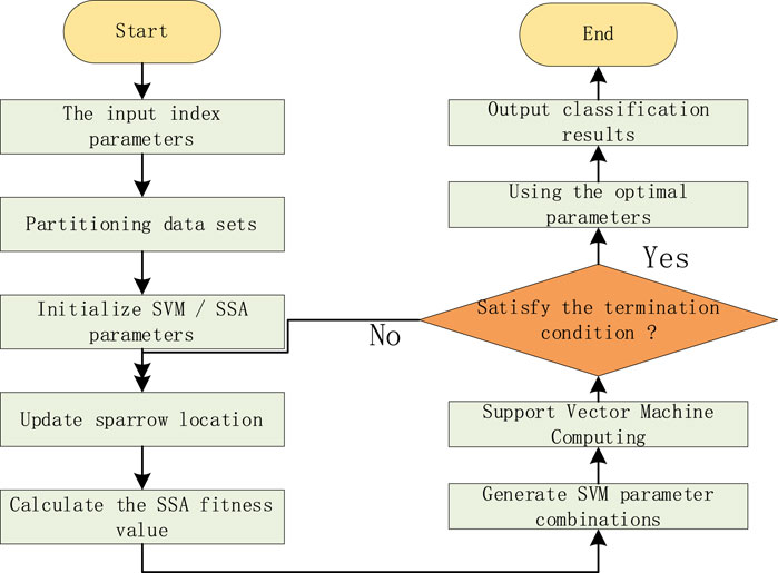
Figure 1. SSA-SVM process.

First, determine the input and output of the fault diagnosis model. Extract fault features as the input of the diagnostic model and determine the target output values. Establish training and testing sample sets. Specifically, the data was divided into training and testing sets with a ratio of 9:1.

Initialize the related parameters of the sparrow search algorithm, including population size, maximum number of iterations, C, and g. Update the position according to Equations 7–9

Calculate the fitness value of the sparrow individual’s new position, compare the updated fitness value with the original optimal value, and update the global optimal information.

Determine whether the number of iterations meets the termination condition. If not, repeat step (3); otherwise, stop, output the optimal parameters, input the test set samples into the optimal SVM model, and output the diagnostic results.

3 Slope stability prediction model based on PCA-SSA-SVM

3.1 Method principle

For the assessment of slope stability, identifying the most prominent influencing factors is imperative. In this research, slopes with a Factor of Safety (FOS) exceeding 1.3 were classified as stable. The stability of slopes is categorized into two groups: stable (coded as 1) and unstable (coded as 0). Historically, slope stability prediction efforts have utilized project data for both training and prediction datasets. However, this often results in a limited amount of training data, leading to suboptimal accuracy in the developed models.

To address this limitation, the present study aggregates numerous referenced engineering cases (Emina et al., 2008; Kardani et al., 2021; Zhang R. et al., 2023; Zhang Y. et al., 2023), amassing a total of 257 experimental datasets to evaluate the model’s efficacy. The comprehensive dataset is presented in Supplementary Table 1. The slope characteristic parameters vary across different slopes. Visual analysis can illustrate the characteristic parameter information of the slope in different states and qualitatively analyze the slope’s condition to some extent.

In evaluating each characteristic parameter, the violin plot shows the distribution of characteristic parameters under different slope conditions, as shown in Figure 2. Among the different characteristic parameters, the violin shapes of the stable and unstable state data are similar, with few or no outliers, indicating that the dataset is reasonably constructed. The data scatter distribution is delineated in Figure 3.

Figure 2

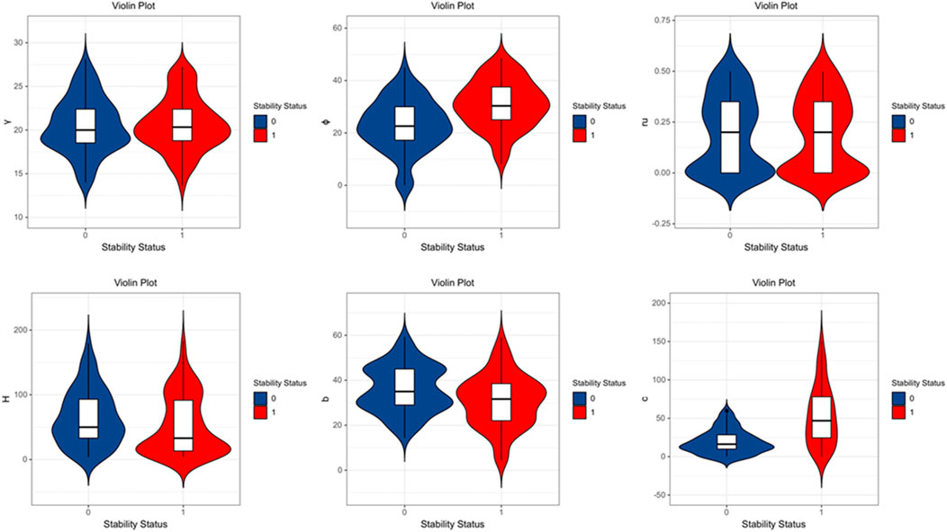
Figure 2. Slope characteristic parameters distribution violin figure.

Figure 3

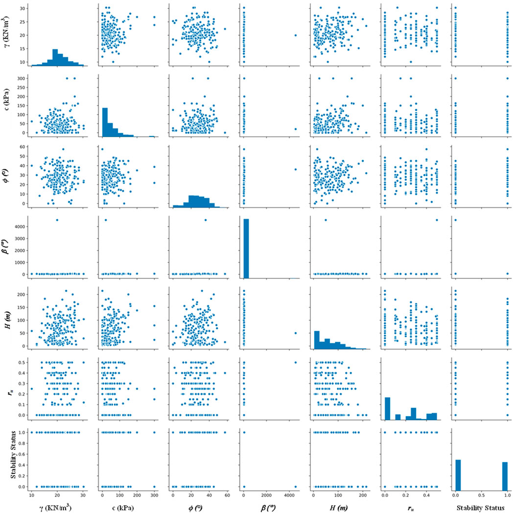
Figure 3. Scatter plot of each index.

To further analyze the data, this paper provides descriptive statistics for six indicators, as shown in Table 1. Given that the total sample size is less than 500, the Shapiro-Wilk (S-W) test is employed to assess the normality of multiple analysis items. The data for the analysis items γ and φ follow a normal distribution. Their median and mean values are close, skewness and kurtosis are near zero, and the significance P-values are 0.051 and 0.052, respectively, which are higher than the commonly used 0.05 significance level, so the null hypothesis of normality cannot be rejected (Sah et al., 1994).

Table 1

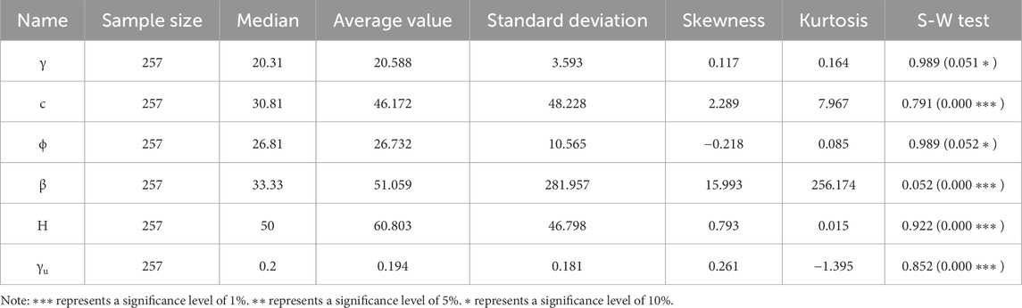
Table 1. Statistical description of samples.

However, the data for c, β, H, and γ_u do not follow a normal distribution. Even though the kurtosis and skewness of H are within the common normal distribution range, the significance P-value remains at 0.000, clearly indicating a departure from normality. Among the six analysis items, two meet the criteria for a normal distribution, while four do not.

Variable correlation analysis is an important part of statistics, which is mainly used to explore whether there is a relationship between two or more variables. In order to prevent data redundancy in the model, which affects the prediction accuracy of the model, the correlation coefficient between the two variables in the data set is calculated to determine whether there are redundant characteristic variables and determine the correlation between variables, see Figure 4. According to the correlation analysis table, it can be observed that there is a positive correlation between γ and c and H, among which the correlation with H is the most significant. c mainly has a strong positive correlation with H, and also has a certain degree of positive correlation with φ. φ shows positive correlation with c and E. The relationship with all other variables is relatively weak, but the positive correlation with ϕ is slightly more obvious. H not only has a significant positive correlation with γ and c, but also has a certain negative correlation with γu. In general, the correlation between H and several other variables is the most prominent, especially the positive correlation with γ, c and the negative correlation with γu; the correlation with all variables is relatively weak.

Figure 4

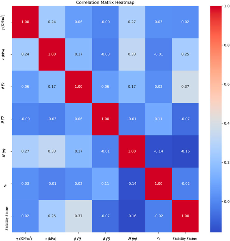
Figure 4. Correlation matrix heat map.

3.2 PCA analysis

In constructing the slope stability prediction model, six key factors related to slope stability status are incorporated. Given the multidimensionality of data derived from these factors, model training becomes challenging. To address this, Principal Component Analysis (PCA) is applied to transform this high-dimensional dataset into a reduced-dimensional space while preserving the original data’s information content as much as possible. This approach helps isolate the most significant principal components, thereby reducing model complexity and enhancing training efficacy. The procedural steps for PCA analysis, as detailed in Section 2.2, are outlined below:

Step 1. Suitability Assessment: Initially, both the Kaiser-Meyer-Olkin (KMO) and Bartlett’s tests are performed to determine the data’s suitability for PCA, as shown in Table 2. A KMO value exceeding 0.8 is optimal, while values between 0.7 and 0.8 are considered moderate. KMO values below 0.6 may be deemed unsuitable. The KMO test results revealed a KMO value of 0.604. Additionally, Bartlett’s sphericity test results showed a significant P-value of 0.000***, which is significant at the respective level. This rejects the null hypothesis, indicating correlations among the variables and affirming the appropriateness of proceeding with PCA.

Table 2

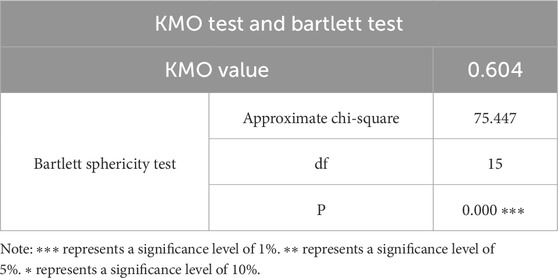
Table 2. PCA feasibility test.

Step 2. Determining the Number of Principal Components: To ascertain the required number of principal components, examine the variance elucidation table and the scree plot. Table 3 lists the variance contribution rate of each principal component to the original variables, which helps in selecting the number of principal components by considering the descending trajectory of eigenvalues. During PCA, the cumulative variance elucidation rate typically approaches 90%. Based on the information in the variance elucidation table, five principal components are identified as input parameters for the SSA-SVM model.

Table 3

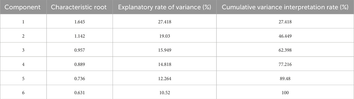
Table 3. Variance interpretation form.

Step 3. Analysis of principal component load coefficient: Table 4 load coefficient combined to reveal the importance of hidden variables behind each principal component.

Table 4

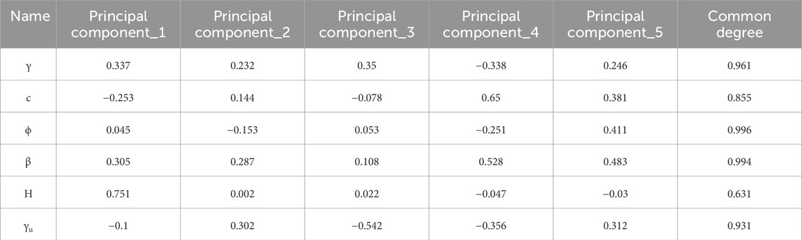
Table 4. Factor load coefficient table.

Step 4. Spatial Representation of Principal Components: The dimensions of numerous principal components are condensed to two or three principal components, and their spatial orientation is depicted using quadrant diagrams. Extracting two or three principal components allows for a clearer visualization of their spatial interrelations. However, since this study extracts five principal components, their spatial distribution cannot be effectively illustrated using the primary mapping technique.

Step 5. Constructing the Principal Component Equation 10: Based on the component matrix, the component formula for each principal component is formulated and its weight is determined, as shown in Table 5.

$\left\{\begin{array}{l}{y}_1=0.367\times \gamma +0.435\times c+0.259\times \varphi -0.015\times \beta +0.456\times H-0.091\times r_u\\ y_2=0.079\times \gamma +0.029\times c+0.305\times \varphi +0.604\times \beta -0.119\times H+0.629\times r_u\\ y_3=0.522\times \gamma +0.108\times c-0.575\times \varphi -0.363\times \beta -0.101\times H+0.537\times r_u\\ y_4=0.254\times \gamma -0.109\times c-0.614\times \varphi +0.705\times \beta +0.199\times H+0.368\times r_u\\ y_5=-0.73\times \gamma +0.770\times c-0.413\times \varphi +0.088\times \beta +0.129\times H+0.196\times r_u\\ y=0.306\times y_1+0.212\times y_2+0.178\times y_3+0.165\times y_4+0.37\times y_5\end{array}\right)(10)$

Table 5

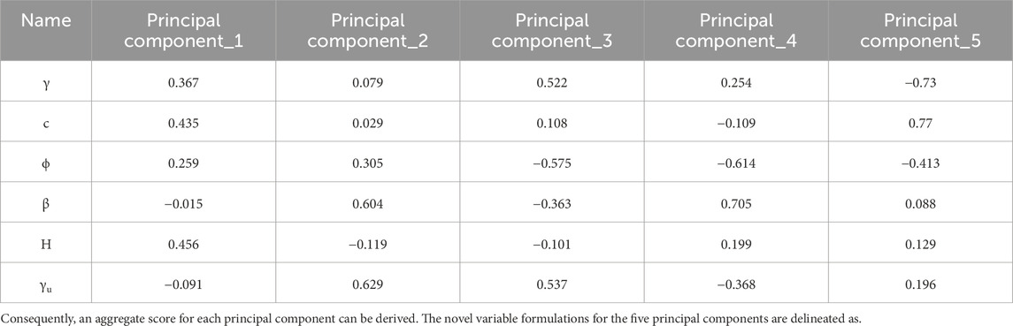
Table 5. Composition matrix table.

Step 6. Comprehensive score output: Finally, calculate and output the comprehensive score based on PCA and the principal component data are shown in Supplementary Table 2.

3.3 PCA-SSA-SVM model construction and training

Utilizing the SSA-SVM approach, an slope stability prediction model is developed. Python software is chosen for scripting the SSA algorithm to enhance the SVM model. After applying principal component analysis (PCA), the initial six evaluation indicators for slope stability are substituted by five principal components. The output variable denotes the safety condition of the slope.

3.4 Model evaluation indicators

The accuracy (ACC), recall rate (TPR), precision rate (PPV) and F1-score were used to evaluate the prediction effect of PCA-SSA-SVM. The calculation formula is, as shown in Equations 11–13 (Khajehzadeh et al., 2022):

$ACC=\frac{TP+TN}{TP+TN+FP+FN}(11)$

$TPR=\frac{TP}{\left(TP+FN\right)}(12)$

$PPV=\frac{TP}{\left(TP+FP\right)}(13)$

TP: True positives, where actual positive samples are correctly predicted as positive; TN: True negatives, where actual negative samples are correctly predicted as negative; FN: False negatives, where actual positive samples are incorrectly predicted as negative; FP: False positives, where actual negative samples are incorrectly predicted as positive.

The F1-score, also referred to as the F-measure, serves as a comprehensive metric that evaluates the model’s precision (PPV) and recall (TPR) as shown in Equation 14. It is computed as the harmonic mean of precision and recall, with values spanning between 0 and 1. A score of 1 indicates impeccable accuracy, while a score of 0 denotes the poorest accuracy.

${{\mathrm{F}}_1}_{-\text{score}}=2\frac{PPV\cdot TPR}{PPV+TPR}(14)$

3.5 Cross-validation

To further enhance the model’s generalization ability and prevent overfitting during the training process, this study employs 5-fold cross-validation, as illustrated in Figure 5. Initially, the original training dataset D is randomly divided into k equally sized subsets: D1, D2, D3, D4, and D5. Let Dj and D-j = D/D_j denote the j-th test set and the corresponding training set, respectively, for each iteration.

Figure 5

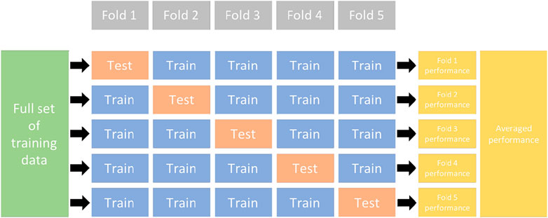
Figure 5. 5-Fold cross-validation.

3.6 Prediction results and analysis

During the data preprocessing phase, the initial dataset was randomly permuted to create a modified dataset. To enhance the model’s generalizability, 231 data entries were designated as the training set, while the remaining entries were reserved for testing. Utilizing the PCA-SSA-SVM approach, a comprehensive prediction was executed on the 257 slope stability data entries. Combining 5-fold cross-validation with model parameter optimization, the results show that the SSA-SVM model’s performance under different parameters indicates that the optimal value for the penalty coefficient (C) in the SVM model is 9.426, and the optimal value for the kernel parameter (gamma) is 0.03.

The exhaustive outcomes are presented in Table 6. The prediction outcomes from the test set are compared with the actual results, with a subsequent analysis conducted in conjunction with the predictions for each state, as depicted in Figure 6.

Table 6

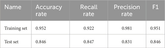
Table 6. Model prediction evaluation.

Based on the data presented in Table 7, the PCA-SSA-SVM model exhibits the highest accuracy, recall, precision, and F1 score compared to the other models. Its accuracy rate is notably high at 84.6%, its recall rate is excellent at 84.7%, and its precision rate is impressive at 83.1%. The SSA-SVM model, with an accuracy rate of 73.1%, a recall rate of 80.1%, and a precision rate of 75%, performs better than the simple SVM model across all metrics, suggesting that incorporating the SSA algorithm improves performance. The PSO-SVM model shows a strong performance with an accuracy rate of 82.5%, a recall rate of 75.3%, and a precision rate of 78.1%, while the GA-SVM model has an accuracy rate of 82.6%, a recall rate of 71%, and a precision rate of 80.2%. Both the PSO-SVM and GA-SVM models exhibit better performance than the SVM model but are slightly lower than the PCA-SSA-SVM model in accuracy and F1 score.

Table 7

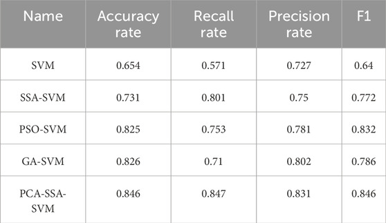
Table 7. Comparison of model predictions using 5-fold cross-validation.

Based on the provided metrics, combining PCA with the SSA algorithm yields the best results among all the models. This integrated approach significantly enhances prediction accuracy and effectiveness, showcasing its superiority in handling high-dimensional data and optimizing model performance. The PCA-SSA-SVM model’s robustness and high precision make it an ideal choice for slope stability prediction in engineering applications.

In order to comprehensively evaluate the performance of the model, this study drew the ROC (receiver operating characteristic) curve and calculated the AUC (area under the curve) value, see Figure 7. The ROC curve is an effective tool for visually demonstrating the relationship between the true positive rate and the false positive rate of the model under various thresholds. The AUC value is the area under the ROC curve, which provides us with a single quantitative indicator of model performance. The AUC value is usually between 0.5 (no discrimination) and 1.0 (perfect discrimination). The model of this study obtained an AUC value of 0.9758, which strongly indicates that the PCA-SSA-SVM model performs well in the slope stability prediction task.

Figure 6

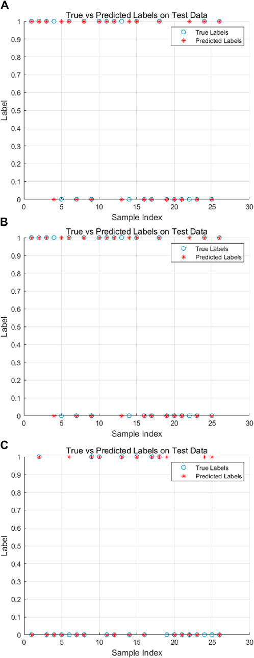
Figure 6. Comparison of model prediction results. (A) SVM (B) SSA-SVM (C) PCA-SSA-SVM.

4 Engineering verification

4.1 Engineering background

The Guangdong Province’s Longchuan to Huaiji Expressway in China is a part of the original national highway network “7,918”plan, specifically marked as the 17th cross route. A significant portion of this route is the Longchuan to Lianping section of the Guangdong Province Longchuan to Huaiji Expressway, commonly referred to as the “LongLian Expressway”. This project is located in the mountainous terrain of northern Guangdong, crossing through Heyuan and Shaoguan cities, encompassing four counties and thirteen towns.

The starting point of the LongLian Expressway is at K206 + 222 in the Old Long Town of Longchuan County, where it connects with the already operational Meihe Expressway. The endpoint is at K334 + 200 in the Tangxia Village, Longxian Town, Wengyuan County, Shaoguan City. The total length of the route is 127.978 km, with a designed speed of 100 km/h, adhering to the technical standards of a two-way four-lane expressway, as shown in Figure 8.

Figure 7

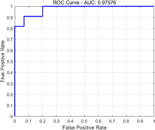
Figure 7. Receiver-operating characteristiccurve.

4.2 Slope profile

4.2.1 Stratigraphic lithology

The surface layer consists of silty clay and sandy clay soil, with plastic to hard plastic consistency. The underlying strata comprise entirely to strongly weathered andesite porphyry and moderately weathered diorite. The fully weathered andesite porphyry is yellow-brown in color, showing complete weathering with substantial disruption of the original rock structure. The core of the rock manifests as hard soil columns, with a soft rock quality that tends to soften and disintegrate when in contact with water, locally interspersed with isolated stones. The strongly weathered andesite porphyry appears yellow, yellow-gray, or yellow-brown, with a major portion of the original rock structure destroyed, exhibiting a medium-grain structure and blocky construction. The mineral composition includes quartz, feldspar, and mica, with the rock core primarily displaying fragmentary and blocky forms, block diameters ranging from 2 to 6 cm, and a minor amount appearing as debris. Joints and fissures are well-developed with some fissure surfaces being impregnated with iron-manganese material, displaying uneven weathering, soft rock quality, and fragmented rock mass. The moderately weathered diorite is gray with a medium to coarse-grain structure and blocky construction. Its mineral composition also includes quartz, feldspar, and mica, with well-developed joints and fissures. The rock core manifests as columnar or short columnar structures, with joint lengths ranging from 10 to 70 cm, producing a brittle sound when struck, indicating hard rock quality and a relatively intact rock mass.

4.2.2 Hydrogeological overview

Surf ace Water: The surface does not exhibit perennial water flow; transient surface runoff only occurs post-rainfall during the rainy season.

Groundwater: The groundwater is composed of upper soil layer pore water and deep bedrock fissure water, with a relatively small water content. The primary source of replenishment relies on the infiltration of atmospheric precipitation, with the discharge base level being the streams at the bottom of the slopes. During the period of this survey, no groundwater levels were detected within the drilled depths.

4.3 Slope data

There are 10 large and small slopes in LongLian Expressway, including 7 unstable slope samples and 3 stable slope samples, as shown in the Table 8.

Table 8

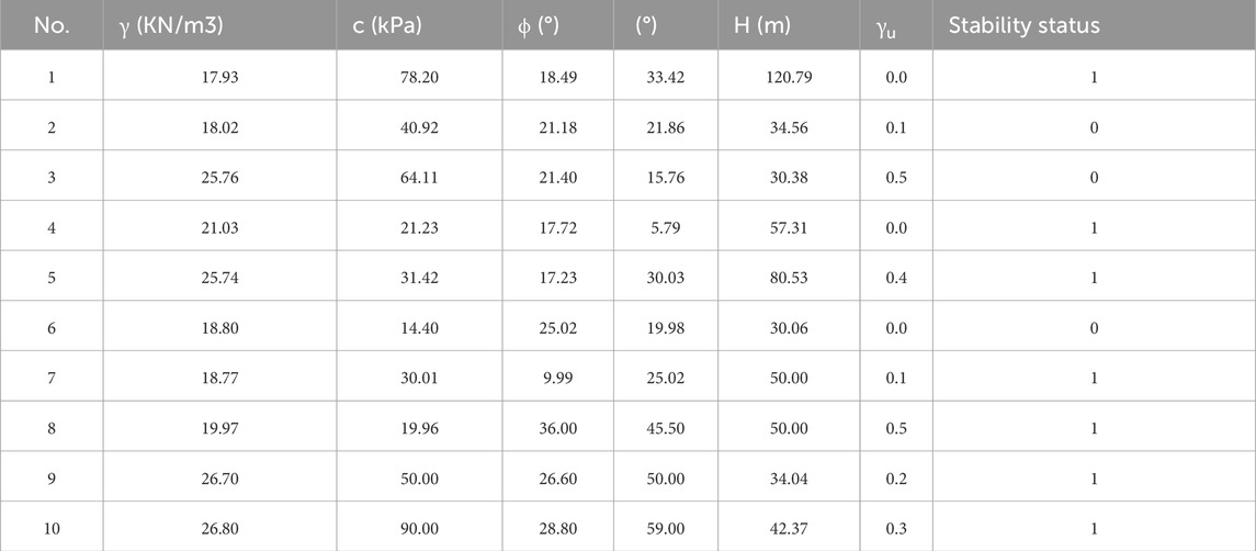
Table 8. Slope data of LongLian Expressway.

4.4 Verification based on PCA-SSA-SVM model

Utilizing the well-trained PCA-SSA-SVM model for slope stability prediction, the results are illustrated in Figure 9. From the provided data, it can be observed that the PCA- SSA-SVM model predictions align with the actual stability status data of the LongLian Expressway slopes at most points. Specifically, among the ten data points, the PCA- SSA-SVM model predictions match the actual stability status at nine points. Only at one data point does the model prediction deviate from the actual stability status.

Figure 8

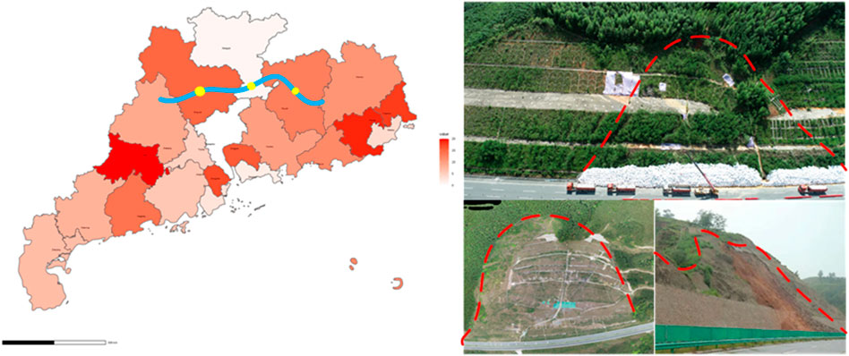
Figure 8. Project location map and slope site.

Figure 9

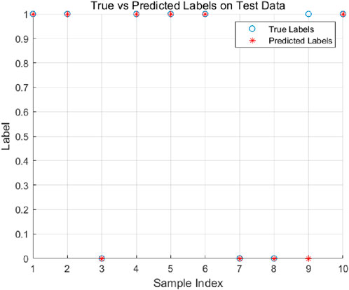
Figure 9. Engineering verification prediction results.

5 Discussion

While the PCA-SSA-SVM model demonstrated high accuracy and robustness, several limitations must be addressed to enhance its applicability and performance in real-world scenarios.

1. Model Limitations: Although the PCA-SSA-SVM model showed excellent performance on the test set, the study does not deeply explore potential limitations in practical applications. The presence of nonlinear relationships between features or potential outliers in the slope dataset may affect the model’s predictive performance. Furthermore, the model’s adaptability to slope data under varying geological conditions or climatic environments requires further investigation.

2. Feature Selection and Optimization: While PCA effectively reduces the dimensionality of the data, the specific rationale for selecting the six features used in this study was not elaborated. Future research should explore feature engineering and optimization techniques to further enhance model predictive performance. Introducing additional features related to slope stability could enrich the model inputs and improve accuracy.

3. Model Comparison and Validation: Although comparisons with SVM and SSA-SVM models were presented, a comparative analysis with other advanced machine learning methods was not included. Future research could investigate the performance of models such as Random Forest, Gradient Boosting Trees, or Deep Learning techniques on the same dataset. Such comparisons would help establish the superiority of the PCA-SSA-SVM model and provide a more comprehensive evaluation of its performance.

6 Conclusion

Within this study, the PCA methodology is employed to examine and process the six evaluative indices affecting slope stability across 257 data samples. From these, five principal components are derived, serving as input variables for the SSA-SVM. Subsequently, a PCA-SSA-SVM predictive model for slope stability is formulated. The accuracy of the model is further evaluated by engineering verification. A detailed analysis of the model’s predictive outcomes and associated errors yielded the subsequent findings.

1. The PCA methodology adeptly addresses the multicollinearity challenge inherent among factors influencing slope stability, streamlining the model’s input variables and enhancing simulation efficiency.

2. The model’s precision, robustness, and adaptability were gauged via metrics such as precision, recall, and the F1-score. The test set outcomes were 84.6%, 84.7%, and 84.6%, respectively. With an AUC value of 0.9758, the model’s accuracy and adaptability are deemed commendable.

3. The accuracy of the PCA-SSA-SVM model was validated using the slope data from the LongLian Expressway. Among the 10 provided samples, only the prediction for sample 1 was incorrect. The results indicate that the PCA-SSA-SVM based slope stability prediction model can be effectively applied in engineering practice to achieve slope stability forecasting.

4. The model’s classification performance has not taken into account factors such as the slope’s geometric shape, soil quality of the slope body, and external influencing elements. Further research is required in the future, especially when using machine learning algorithms to estimate slope stability, to continue refining and enhancing feature parameters.

Data availability statement

The original contributions presented in the study are included in the article/supplementary material, further inquiries can be directed to the corresponding author.

Author contributions

JH: Investigation, Methodology, Software, Writing–original draft. DL: Conceptualization, Data curation, Formal Analysis, Investigation, Methodology, Resources, Writing–original draft, Writing–review and editing. WL: Writing–original draft. QY: Writing–review and editing.

Funding

The author(s) declare that no financial support was received for the research, authorship, and/or publication of this article.

Conflict of interest

Authors JH, WL, and QY were employed by Guangxi Geology and Mineral Construction Group Co., Ltd. Author DL was employed by Guangxi Shengfeng Construction Group Co. Ltd.

Publisher’s note

All claims expressed in this article are solely those of the authors and do not necessarily represent those of their affiliated organizations, or those of the publisher, the editors and the reviewers. Any product that may be evaluated in this article, or claim that may be made by its manufacturer, is not guaranteed or endorsed by the publisher.

Supplementary material

The Supplementary Material for this article can be found online at: https://www.frontiersin.org/articles/10.3389/feart.2024.1429601/full#supplementary-material

References

Bu, N., Zhao, H., and Xie, J. (2009). Slope stability analysis with DE-BP neural network. Subgr. Eng. (4), 2.

Google Scholar

Chen, J., Zheng, R., and Chen, H. (2014). Slope stability analysis based on PCA and BP neural network. China Saf. Sci. J. 10 (5), 6.

Google Scholar

Ding, H., Zhu, J., and Luo, S. (2011). Research on slope stability prediction model based on PCA-SVM. Subgr. Eng. (2), 3.

Google Scholar

Duncan, J. M. (1996). State of the art: limit equilibrium and finite-element analysis of slopes. J. Geotechnical Eng. 123 (7), 577–596. doi:10.1061/(asce)0733-9410(1996)122:7(577)

CrossRef Full Text | Google Scholar

Emina, E., Torlakovic, , Driman, D. K., Parfitt, J. R., Wang, C., Benerjee, T., et al. (2008). Sessile serrated adenoma (SSA) vs. traditional serrated adenoma (TSA). Am. J. Surg. Pathology 32, 21–29. doi:10.1097/pas.0b013e318157f002

PubMed Abstract | CrossRef Full Text | Google Scholar

Gu, Q., Cai, Z. H., Zhu, L., and Huang, B. (2009). Slope stability prediction based on PCA-GEP algorithm. Rock Soil Mech. 30 (3), 757–761 + 768. doi:10.3969/j.issn.1000-7598.2009.03.033

CrossRef Full Text | Google Scholar

Hu, J., Cheng, P., and Liu, M. M. (2021). Numerical modeling of 3D slopes with weak zones by random field and finite elements. Appl. Sci. 11, 9852. doi:10.3390/app11219852

CrossRef Full Text | Google Scholar

Jin, A., Zhang, J., Sun, H., and Wang, B. (2022). An intelligent prediction and early warning model for slope instability based on SSA-SVM. J. Huazhong Univ. Sci. Technol. Nat. Sci. Ed. 50 (11), 142–148. doi:10.13245/j.hust.221118

CrossRef Full Text | Google Scholar

Kardani, N., Zhou, A., Nazem, M., and Shen, S. L. (2021). Improved prediction of slope stability using a hybrid stacking ensemble method based on finite element analysis and field data. J. Rock Mech. Geotechnical Eng. 13 (1), 188–201. doi:10.1016/j.jrmge.2020.05.011

CrossRef Full Text | Google Scholar

Khajehzadeh, M., Taha, M. R., Keawsawasvong, S., Mirzaei, H., and Jebeli, M. (2022). An effective artificial intelligence approach for slope stability evaluation. IEEE Access 10, 5660–5671. doi:10.1109/access.2022.3141432

CrossRef Full Text | Google Scholar

Li, N., Wang, Y., and Ma, W. (2022). A wind power prediction method based on DE-BP neural network[J]. Front. energy res. 10, 844111. doi:10.3389/fenrg.2022.844111

CrossRef Full Text | Google Scholar

Lu, P., and Rosenbaum, M. (2003). Artificial neural networks and grey systems for the prediction of slope stability. Nat. Hazards 30 (3), 383–398. doi:10.1023/b:nhaz.0000007168.00673.27

CrossRef Full Text | Google Scholar

Luan, B., Zhou, W., Jiskani, I. M., Lu, X., and Wang, Z. (2023). Slope stability prediction method based on intelligent optimization and machine learning algorithms. Sustainability 15, 1169. doi:10.3390/su15021169

CrossRef Full Text | Google Scholar

Moayedi, H., Bui, D. T., Kalantar, B., and Kok Foong, L. (2019). Machine-learning-based classification approaches toward recognizing slope stability failure. Appl. Sci. 9 (21), 4638. doi:10.3390/app9214638

CrossRef Full Text | Google Scholar

Sah, N., Sheorey, P., and Upadhyaya, L. (1994). Maximum likelihood estimation of slope stability. Int. J. Rock Mech. Min. Sci. and Geomechanics Abstr. 31 (1), 47–53. doi:10.1016/0148-9062(94)92314-0

CrossRef Full Text | Google Scholar

Sloan, S. W. (1989). Upper bound limit analysis using finite elements and linear programming. Int. J. Numer. Anal. Methods Geomechanics 13 (3), 263–282. doi:10.1002/nag.1610130304

CrossRef Full Text | Google Scholar

Suman, S., Khan, S. Z., Das, S. K., and Chand, S. K. (2016). Slope stability analysis using artificial intelligence techniques. Nat. Hazards 84 (2), 727–748. doi:10.1007/s11069-016-2454-2

CrossRef Full Text | Google Scholar

Wang, G. J., Zhao, B., Wu, B., Zhang, C., and Liu, W. (2022). Intelligent prediction of slope stability based on visual exploratory data analysis of 77 in situ cases. Int. J. Min. Sci. Technol. doi:10.1016/j.ijmst.2022.07.002

CrossRef Full Text | Google Scholar

Wei, W., Li, X., Liu, J., Zhou, Y., and Zhou, J. (2021). Performance evaluation of hybrid WOA-SVR and HHO-svr models with various kernels to predict factor of safety for circular failure slope. Appl. Sci. 11 (4), 1922. doi:10.3390/app11041922

CrossRef Full Text | Google Scholar

Xie, W., Nie, W., Saffari, P., Robledo, L. F., Descote, P. Y., and Jian, W. (2021). Landslide hazard assessment based on Bayesian optimization–support vector machine in Nanping City, China. Nat. Hazards 109 (1), 931–948. doi:10.1007/s11069-021-04862-y

CrossRef Full Text | Google Scholar

Xu, C., Xu, X., Dai, F., Wu, Z., He, H., Shi, F., et al. (2013). Application of an incomplete landslide inventory, logistic regression model and its validation for landslide susceptibility mapping related to the may 12, 2008 wenchuan earthquake of China. Nat. Hazards 68 (2), 883–900. doi:10.1007/s11069-013-0661-7

CrossRef Full Text | Google Scholar

Zhang, H., Wu, W., Zhang, X., Han, L., and Zhang, Z. (2023). Slope stability prediction method based on the margin distance minimization selective ensemble. Catena 2023-08-20. doi:10.1016/j.catena.2022.106055

CrossRef Full Text | Google Scholar

Zhang, R., Su, J., and Feng, J. (2023a). An extreme learning machine model based on adaptive multi-fusion chaotic sparrow search algorithm for regression and classification. Evol. Intell. 17, 1567–1586. doi:10.1007/s12065-023-00852-0

CrossRef Full Text | Google Scholar

Zhang, S., Zheng, D., and Zhang, W. (2022b). A rapid evaluation method for the stability of red-layer highway slopes based on the SVM algorithm. Northwest Hydropower, (000-003). doi:10.3969/j.issn.1006-2610.2022.03.001

CrossRef Full Text | Google Scholar

Zhang, W., Li, H., Han, L., Chen, L., and Wang, L. (2022a). Slope stability prediction using ensemble learning techniques: a case study in yunyang county, chongqing, China. J. Rock Mech. Geotech. Eng. 14 (4), 1089–1099. doi:10.1016/j.jrmge.2021.12.011

CrossRef Full Text | Google Scholar

Zhang, Y., Ding, J., Sun, J., and Zhang, D. (2023b). Prediction and online optimization of strip shape in hot strip rolling process using sparrow search algorithmonline sequential deep multilayer extreme learning machine algorithm. Steel Res. Int. 94. doi:10.1002/srin.202200832

CrossRef Full Text | Google Scholar

Zienkiewicz, O. C., Humpheson, C., and Lewis, R. W. (1975). Associated and non-associated visco-plasticity and plasticity in soil mechanics. Géotechnique 25 (4), 671–689. doi:10.1680/geot.1975.25.4.671

CrossRef Full Text | Google Scholar