Numerical simulation of groundwater in hyporheic zone with coupled parameter stochastic scheme

Groundwater numerical modeling is a crucial scientific tool for understanding groundwater circulation and supporting regional water resource planning and management. The effectiveness of these models depends largely on the accuracy of hydrogeological parameters within aquifers, which are often spatially heterogeneous and randomly distributed due to complex geological and tectonic factors. Traditional modeling approaches frequently overlook this randomness, compromising the precision and resolution of groundwater simulations. This study focuses on a section of the Qingshui River in the Huaihe River Basin. Using field and laboratory data, probability distribution functions for key parameters like hydraulic conductivity, specific yield, and specific storage were developed. These functions were integrated into the groundwater model to reflect the inherent stochastic nature of aquifer properties. This integration significantly enhanced model accuracy, reducing the root mean square error of simulated water levels from 0.47–1.43 m to 0.13–0.16 m and improving the Nash-Sutcliffe efficiency coefficients (NSE) from −2.96–0.73 to 0.94–0.98. Additionally, the model facilitated analysis of the interactions between river and groundwater, particularly in the hyporheic zone, under various scenarios. It identified spatial and temporal variations in groundwater recharge dynamics and delay effects at different distances from the river channel. For instance, recharge rates at 50 m and 150 m from the river were 0.295 m/day and 0.015 m/day, respectively, indicating stronger recharge closer to the river. The study also assessed the impact of varying river flows, riverbed permeability, and irrigation practices on water exchanges between the river and groundwater. These factors were found to significantly influence the intensity of water exchange, seepage, and groundwater reserves. This research provides valuable insights for managing river-groundwater interactions and analyzing the ecological environment of surrounding groundwater systems, underscoring the importance of incorporating stochastic characteristics into groundwater modeling.

1 Introduction

The hyporheic zone represents an area where surface and groundwater interactions are most frequent and intense. Facilitated by dual water sources, this zone typically maintains a relatively abundant and stable water supply. Such hydrological dynamics hold significant implications for the evaluation, development, and management of water resources. Moreover, the riparian ecosystems fostered within this zone often exhibit crucial ecological functions and value, particularly in arid regions (Wang et al., 2023). Consequently, the interplay between river and groundwater within the hyporheic zone has garnered considerable multidisciplinary attention (Wang, 2018; Zhang et al., 2020). Nevertheless, the sedimentary environment of the hyporheic zone is intricately complex, compounded by strong spatial heterogeneity within the aquifer. The challenge lies in scientifically and accurately describing the hydrogeological parameters, which ultimately constrains our understanding of this intricate relationship.

Hydrogeological parameters serve as indicators that characterize the permeability, water storage, or water release properties of aquifers or aquifer media. They are pivotal parameters for simulating the quantitative movement characteristics of groundwater (Ya, 2019; Kumar et al., 2022; Zhao et al., 2022). Due to the complex formation processes of the strata, hydrogeological characteristics exhibit strong spatial heterogeneity, manifesting stochastic distribution characteristics on a large scale (Ramadas et al., 2015; Zhang et al., 2020; JI et al., 2023). In traditional numerical simulations of groundwater, the hydrogeological parameters for a large area are typically determined based on the experimental results of individual locations, neglecting the stochastic characteristics of the parameters, resulting in certain shortcomings in the efficiency of model parameter calibration and the description of the groundwater flow field (Yang et al., 2021; Liu et al., 2023; Lyu et al., 2024; Schiavo, 2024). To depict the spatial variability of hydrogeological parameters, some scholars have explored the relationship between parameter statistical characteristics and probability distribution functions based on the theory of parameter random distribution (Ji et al., 2021; Ni et al., 2021). They transform the parameters of porous media into a stochastic field model, thereby utilizing probability functions to quantify the uncertainty of water flow characteristics and solute transport features (Zhu et al., 2019).

The theory of random fields (RFT) addresses the deficiency of traditional probability theory, which treats geotechnical parameters as a single random variable, resulting in the loss of structural information within the spatial domain. By considering the autocorrelation of soil parameters, it describes the physical properties of soil using spatial random fields. This concept was first introduced by Cornell (1972), and subsequently refined by Wu (1974) and Lumb (1975). They established a random field model that reflects the spatial autocorrelation characteristics of geotechnical parameters. Building on the work of predecessors, Vanmarcke (1977) further proposed the concept of autocorrelation distance and its calculation method, successfully characterizing and predicting the natural variability characteristics of soil properties, providing an effective approach for the application of RFT in geotechnical engineering analysis and computation. RFT has been extensively applied in the study of the hydrologic properties of soil (e.g., Srivastava et al., 2010; Lei et al., 2016), pore water pressure, seepage characteristics of slopes, and their stability analysis (e.g., Li et al., 2009; Santoso et al., 2011; Cho, 2012; Zhu et al., 2013).

While scholars have conducted extensive research on the RFT of soil parameters, the practical application of relevant research findings has primarily been within the realm of engineering geological rock and soil stability (Yuan et al., 2020). However, in numerical groundwater simulations, a fixed parameter is typically assigned to a given aquifer, often overlooking its spatial heterogeneity and frequency distribution characteristics. Recent studies have found that the spatial heterogeneity and stochastic characteristics of aquifer parameters have significant impacts on the parameter calibration efficiency and simulation accuracy of numerical models. For instance, Tang et al. (2017) observed that the random distribution characteristics of riverbed hydrogeological parameters significantly impact the accuracy of simulating river-groundwater interactions, and Schiavo (2024) improved the model convergence by using the Monte Carlo algorithm considering the heterogeneity of aquifer conductivity, indicating limitations in the traditional homogeneous aquifer assumption for studying small-scale and high-precision hyporheic zones (Shu et al., 2024).

Hydraulic conductivity (K), specific storage (S_s), and specific yield (S_y), as important hydrogeological parameters that reflect the hydraulic characteristics of aquifers, directly affect the characteristics of groundwater seepage and storage, as well as the degree of hydraulic connection between rivers and groundwater (Prajapati et al., 2021). They have a significant impact on the key calculations of water exchange between rivers and groundwater and on the research of groundwater ecological effects (Bonanno et al., 2021; Cao et al., 2021). Therefore, how to depict the probability distribution characteristics of hydrogeological parameters to more reasonably delineate hydrogeological units has been a research hotspot in recent years and is of great significance to the study of the mutual replenishment relationship between rivers and groundwater (Zhao et al., 2012; Cao et al., 2013; Rezapour and Yazdi, 2014).

This study relies on field monitoring and laboratory analysis experiments conducted in a typical reach of the Qingshui River in the Huai River Basin. Based on particle size distribution tests, soil sample properties were classified, and corresponding soil parameters obtained from geological surveys were combined with laboratory test results of soil hydraulic properties to establish probability distribution models for hydraulic conductivity, specific storage, and specific yield. Subsequently, a groundwater numerical model was established to analyze the effect of the parameter random distribution model on improving the accuracy of groundwater numerical simulations and to investigate the mechanisms of interaction between subsurface flow and river water. The research results will contribute to deepening the theory of stochastic hydrological simulation of groundwater and providing technical support for the operation of the Yangtze-to-Huaihe Water Diversion Project (YHWDP).

2 Materials and methods

2.1 Overview of the study area

The study area is located in the Qingshui River section of the YHWDP (Figure 1). This project connects the Yangtze River and the Huaihe River, offering significant benefits such as ensuring water supply, facilitating shipping, and improving the water environment. Primarily focused on urban and rural water supply, it also aims to enhance the local water ecological environment. Classified as a grade I project. The study area is situated in the Yellow-Huai Alluvial Plain. The Qingshui River has a total length of 137.3 km, with a basin area of 901 km². Within Henan Province, the river’s length is 88.4 km, covering a basin area of 548 km².

Figure 1

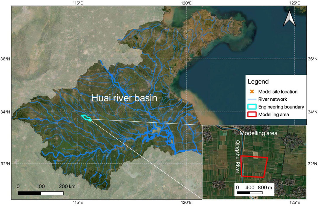
Figure 1. Research area geographic information map.

Characterized by a warm temperate semi-humid continental monsoon climate, the study area experiences seasonal variations in temperature, precipitation, and wind direction. Annual precipitation averages between 720 and 820 mm, with significant variability throughout the year. The rainy season, spanning from June to September, typically contributes to over 70% of the annual rainfall. Additionally, interannual rainfall variations are considerable, with differences between maximum and minimum rainfall ranging from 2 to 4 times. Average annual evaporation rates range from 1,200 to 1,400 mm in the upper reaches and reach 1866 mm in the middle and lower reaches.

The simulation area is situated within the key monitoring section 16 of the Qingshui River segment. Groundwater within the area is primarily characterized as Quaternary loose layer pore phreatic water, predominantly occurring in sandy loam, light silty loam, and fine sand layers, with the lower fine sand layer being pressure-bearing. Sandy loam and silty fine sand exhibit moderate water permeability, while light silty loam displays weak to moderate permeability. Heavy silty loam, on the other hand, acts as a relative aquiclude with weak water permeability.

Throughout the exploration period, groundwater depths typically range between 3 and 5 m, displaying dynamic characteristics within a range of 1–3 m. The main sources of groundwater recharge within the site include atmospheric precipitation, river infiltration, and lateral groundwater recharge, while the main discharge pathways include evaporation, pumping, lateral runoff, and river discharge. With the variations in precipitation and the impact of water transfer projects, the exchange between river water and groundwater in the area shows significant variability. When the river level is high, river water recharges the groundwater; conversely, when the river water level is low, groundwater replenishes the river water.

2.2 Data collection and monitoring

2.2.1 Hydrogeological data collection and analysis

The hydrogeological and engineering geological conditions, as well as the digital elevation model (DEM) data along the river course in the study area, were derived from a comprehensive analysis of the engineering geological survey report and atlas conducted during the feasibility study stage of the water supply supporting project in Henan Province. This analysis encompassed data from the water diversion area, extending from the Yangtze River to the Huaihe River, as well as on-site geological drilling data. Surface conditions were primarily obtained through remote sensing satellites and on-site unmanned aerial vehicles. Additionally, the DEM digital elevation model of the study area was generated using ArcGIS software to furnish precise surface data for the groundwater model.

2.2.2 Aquifer hydraulic parameters test

To ascertain the spatial distribution characteristics of the permeability coefficient within the stratum, 3×3 soil geological boreholes were conducted along both horizontal and vertical directions (Figure 2). Permeable sand layers were encountered at varying vertical depths. Sampling was performed at vertical intervals of 0.5 m–1.0 m, with soil samples collected and tested for parameters including density, particle size, specific yield, and permeability coefficient at each layer. The technical flow chart of the aquifer water test is illustrated in Figure 3.

Figure 2

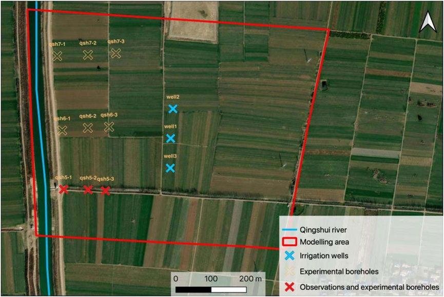
Figure 2. Field monitoring and drilling schematic diagram.

Figure 3

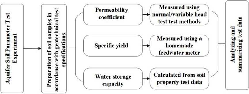
Figure 3. Flow chart of aquifer hydraulic test technology.

2.2.2.1 Determination of hydraulic conductivity

Using the MS2000 laser particle size analyzer from the UK, supplemented by the EVO 18 geochemical analyzer from Germany, particle size and mineralogical analyses were conducted to obtain the percentages of clay, silt, and sand in soil samples, as well as the mineralogical composition of the samples.

In this study, the SLB-1 type stress-strain controlled triaxial permeameter was used to more accurately simulate the permeability characteristics of soil under certain confining pressure conditions. For coarse-grained and fine-grained soil samples, constant head and falling head permeability tests were conducted, respectively.

2.2.2.2 Determination of water yield

Water yield serves as a crucial parameter in various hydrological calculations, including the water balance assessment of shallow groundwater resources, the analysis of unsteady groundwater flow, the computation of groundwater level decline in agricultural drainage, and investigations into the interconversion of atmospheric water, surface water, and groundwater.

Specific yield, on the other hand, represents the ratio of water volume to the volume of porous media that can be released by the saturated medium due to gravity drainage. In this study, a custom-made specific yield meter was utilized to saturate undisturbed soil, allowing it to freely drain under the influence of gravity. This enabled the determination of the discharged water volume, thereby deducing the specific yield of the undisturbed soil.

2.2.3 Groundwater level monitoring

To investigate the interaction between river and groundwater, three automatic observation wells were installed perpendicular to the river channel at distances of 50 m, 100 m, and 150 m from the river. These observation wells were equipped with VWP-0.35G groundwater level sensors developed by Nanjing Genanyun Company, with monitoring conducted at a frequency of once every 24 h. Given that farmland is the predominant land use type in the study area and numerous irrigation wells are present in the vicinity, manual patrols were conducted in addition to automatic monitoring. These patrols enabled regular assessments of groundwater extraction activities in the surrounding areas.

2.3 Visual MODFLOW flex model

The United States Geological Survey (USGS) released the Modular Three-Dimensional Finite-Difference Ground-Water Flow Model (i.e., MODFLOW) model in 1981, which utilizes a modular model structure to depict different groundwater processes and is one of the most widely used models in the field of groundwater simulation research. The groundwater numerical simulation software in this study employs the Visual MODFLOW Flex model developed by Waterloo Hydrogeologic Company in Canada based on MODFLOW. Visual MODFLOW Flex is a widely utilized professional software system designed for simulating and evaluating solute transport and visualizing three-dimensional groundwater flow. The model is employed to simulate groundwater flow in aquifers with specified boundary conditions. It facilitates the easy assignment of values to each partition unit and boundary conditions, rapid output of model areas and division of calculation units, and provides visual output of simulation results.

The MODFLOW model is a three-dimensional unsteady flow mathematical model, which corresponds to the hydrogeological conceptual model of the groundwater system in the study area. It combines the seepage continuity equation and Darcy’s law, with the finite difference method applied to decompose the groundwater partial differential equation (Eq. 1). This approach allows for the utilization of various mathematical models to describe groundwater flow movement.

$\left\{\begin{array}{l}\frac{\partial }{\partial x}\left(K_{xx}\frac{\partial H}{\partial x}\right)+\frac{\partial }{\partial y}\left(K_{yy}\frac{\partial H}{\partial y}\right)+w=\mu \frac{\partial H}{\partial t}\left(x,y\right)\in \mathrm{\Omega }\\ {\left.H\left(x,y,t\right)\right|}_{t=0}=H0\left(x,y\right)\left(x,y\right)\in \mathrm{\Omega }\\ {\left.K_n\frac{\partial H}{\partial n}\right|}_{S_2}=q\left(x,y,t\right)\left(x,y\right)\in S_2\end{array}\right.(1)$

In Eq. 1, Ω represents the groundwater flow domain, H denotes the hydraulic head of the aquifer (m). $S_2$ represents the type 2 boundary of the model, while $K_{xx}$ and $K_{yy}$ are the hydraulic conductivities in the x and y directions, respectively (m/d). W represents the source/sink terms, which may include rainfall infiltration, evaporation, etc. Additionally, μ represents the specific yield of the aquifer, while $H0\left(x,y\right)$ represents the initial hydraulic head function (m). The term $q\left(x,y,t\right)$ represents the type 2 boundary unit-area flow function (m/d), and n represents the outward normal direction of each boundary face.

Based on the hydrogeological conditions and observational data of the study area boundary, the lateral boundary is characterized as a constant head boundary. The upper boundary corresponds to the phreatic surface, influenced by precipitation infiltration and human activities such as mining. The lower boundary consists of Tertiary strongly weathered argillaceous sandstone, generalized as a water-resisting boundary. Recharge primarily comprises lateral inflow and rainfall infiltration, while discharge mainly encompasses artificial mining and lateral outflow.

2.4 Multi-parameter probability distribution theory

According to field and laboratory test data, parameters such as permeability coefficient, specific yield, and water storage coefficient in the study area were analyzed individually. Characteristic values of these parameters were obtained by establishing probability distribution functions as input values for hydrogeological parameters. Subsequently, the accuracy of the groundwater numerical model based on multi-parameter probability distribution was analyzed.

Given the characteristics of random variables, they are typically categorized into discrete and continuous types. Continuous random variables primarily depict continuous geological phenomena, such as porosity, permeability coefficient, and saturation. Parameters like permeability coefficient, specific yield, and water storage rate exhibit traits of continuous random variables, for which various continuous distribution density functions can be chosen to generate parameter fields. Common continuous distribution density functions encompass uniform distribution, exponential distribution, normal distribution, and t distribution, among others. Notably, the normal distribution, also known as Gaussian distribution, holds significant importance in mathematics, physics, and engineering, exerting substantial influence across diverse statistical contexts. Denoted by X∼N(μ,σ²) for mathematical expectation and variance, the probability density function and cumulative distribution function of normal distribution are represented as follows (Eqs 2, 3):

$f\left(x\right)=\frac{1}{\sqrt{2\pi }\sigma }{e}^{-\frac{{\left(x-\mu \right)}^2}{2{\sigma }^2}},-\infty <x<+\infty (2)$

$F\left(x\right)=\frac{1}{\sqrt{2\pi \sigma }}{\int }_{-\infty }^x{e}^{-\frac{{\left(y-\mu \right)}^2}{2{\sigma }^2}}dy(3)$

The t-distribution is employed to estimate the mean of a population with a normal distribution and unknown variance, particularly when dealing with small samples. When the overall variance is known, such as in the case of large sample sizes, the normal distribution is more appropriate for estimating the overall mean. The shape of the t distribution curve is influenced by the degrees of freedom n. Compared to the standard normal distribution curve, t distribution curves tend to be flatter with lower peaks in the middle and higher tails on both sides, with smaller degrees of freedom resulting in flatter curves and more pronounced tails. As the degree of freedom n increases, the t-distribution curve converges closer to the normal distribution curve. Specifically, when the degree of freedom is large, the t distribution curve approaches the standard normal distribution curve. Now, assuming X follows a standard normal distribution and Y follows a chi-square distribution, their distribution yields the t distribution with n degrees of freedom, denoted by Z∼t(n). Additionally, if k mutually independent random variables adhere to the standard normal distribution, the sum of squares of these k random variables forms a new random variable X, whose distribution is termed as chi-square distribution, denoted by Q∼χ(n), where n represents the degree of freedom. The distribution density function of the t distribution is shown in Eq. 4.

$f\left(x\right)=\frac{\text{Gam}\left(\frac{n+1}{2}\right)}{\sqrt{n\pi }\text{Gam}\left(\frac{n}{2}\right)}{\left(1+\frac{x^2}{n}\right)}^{-\frac{n+1}{2}}(4)$

Here, Gam (x) is the gamma function.

The probability density function (Eq. 5) and cumulative distribution function (Eq. 6) of the exponential distribution are as follows:

$f\left(x\right)=\left\{\begin{array}{l}\frac{1}{\theta }{e}^{-\frac{x}{\theta }},x>0\\ 0,x\le 0\end{array}\right.\left(\theta >0\right)(5)$

$F\left(x\right)=\left\{\begin{array}{l}1-e^{-\theta x},x\ge 0\\ 0,x<0\end{array}\right.\left(\theta >0\right)(6)$

The one-sample Kolmogorov-Smirnov (K-S) test is employed to assess whether a sample originates from a particular theoretical distribution. This test compares the cumulative frequency distribution of the sample data with the specified theoretical distribution. A small discrepancy between the two suggests that the sample aligns with the specified distribution. The criterion for significance in the one-sample K-S test is crucial. If the significance value exceeds 0.05, it can be inferred that the sample is drawn from the specified distribution.

2.5 Model accuracy assessment

2.5.1 Nash-Sutcliffe efficiency coefficient

In Eq. 7, ${\mathrm{i}}_{\mathrm{T}}$ represents the total number of measured or calculated heads. When NSE = 1, it indicates a perfect fit between the measured value and the calculated value;

$\text{NSE}=\frac{{\displaystyle {\sum }_{\mathrm{i}=1}^{{\mathrm{i}}_{\mathrm{T}}}}{\left({\mathrm{h}}_{\mathrm{i}}-{\mathrm{H}}_{\mathrm{i}}\right)}^2}{{\displaystyle {\sum }_{\mathrm{i}=1}^{{\mathrm{i}}_{\mathrm{T}}}}{\left({\mathrm{H}}_{\mathrm{i}}-{\overline{\mathrm{H}}}_{\mathrm{i}}\right)}^2}(7)$

In this context, ${\mathrm{H}}_{\mathrm{i}}$ represents the actual water head observation value of the observation hole in meters, ${\mathrm{h}}_{\mathrm{i}}$ denotes the calculated value of the head of the numerical model in meters, ${\overline{\mathrm{H}}}_{\mathrm{i}}$ signifies the average value of the actual water head observation of the observation hole, also measured in meters.

2.5.2 Root mean square error

The root mean square error (RMSE) is calculated as the square root of the ratio of the sum of squared deviations between the predicted values and the actual values to the number of observations n (Eq. 8). It serves to quantify the degree of deviation of the measured data from the real values. A smaller RMSE value indicates higher measurement accuracy.

$\text{RMSE}=\sqrt{\frac{1}{\mathrm{m}}{\displaystyle {\sum }_{\mathrm{i}=1}^{\mathrm{m}}}{\left({\mathrm{y}}_{\mathrm{i}}-{\widehat{\mathrm{y}}}_{\mathrm{i}}\right)}^2}(8)$

where, ${\mathrm{y}}_{\mathrm{i}}$ represents the actual water head observation value of the observation hole in meters, while ${\widehat{\mathrm{y}}}_{\mathrm{i}}$ signifies the calculated value of the head of the numerical model, also measured in meters.

2.5.3 Coefficient of determination

${\mathrm{R}}^2$ serves as a metric to assess the goodness of fit of linear regression models in statistics (Eq. 9). Its value falls within the range of 0–1. A value closer to 1 indicates a better fitting effect.

${\mathrm{R}}^2=1-\frac{{\displaystyle \sum _{\mathrm{i}}}{\left({\widehat{\mathrm{y}}}_{\mathrm{i}}-{\mathrm{y}}_{\mathrm{i}}\right)}^2}{{\displaystyle \sum _{\mathrm{i}}}{\left({\overline{\mathrm{y}}}_{\mathrm{i}}-{\mathrm{y}}_{\mathrm{i}}\right)}^2}(9)$

where, ${\mathrm{y}}_{\mathrm{i}}$ represents the actual water head observation value of the observation hole in meters; ${\widehat{\mathrm{y}}}_{\mathrm{i}}$ denotes the calculated value of the head of the numerical model, also measured in meters; ${\overline{\mathrm{y}}}_{\mathrm{i}}$ signifies the average value of the actual water head observation of the observation hole, also measured in meters.

3 Construction of groundwater numerical model

3.1 Conceptual model

The generalized scope of this model does not represent an independent, complete hydrogeological unit. To facilitate numerical simulation, the west boundary is delineated by the Qingshui River, with the given head boundary set according to the river level. Spanning 650 m from north to south, the model boundary aligns with the vertical direction of the river. Considering the groundwater flow network’s characteristics, it is designated as the zero-flow boundary. On the east, the boundary is demarcated by the serialized monitoring well, designated as the specified water head boundary based on groundwater survey records, accounting for minimal irrigation during the study period. Based on borehole disclosures, the study area is predominantly composed of silty clay, heavy silty loam, and loam, with clay and sandy loam distributed in thin layers or lenticular shapes. Consequently, in the vertical direction, the model aquifer is divided into layers I, II, III, and IV.

Taking into account both calculation workload and accuracy requirements, we’ve set the spatial resolution of the model to 5 m, with a simulation time resolution set at the daily scale. The model is subdivided into 121 rows and 185 columns, resulting in a total of 82,200 rectangular grid elements (Figure 4). Calculation nodes are positioned at the center of each unit. The simulation commenced on 26 August 2022, and spans 8 months based on daily time increments.

Figure 4

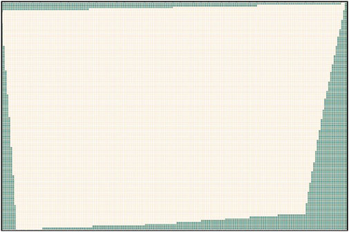
Figure 4. Mesh generation for the model.

3.1.1 Hydrogeologic parameters

Based on the hydrogeological conditions of the study area, combined with hydrogeological data and experimental test results, it was found that the hydrogeologic parameters in the study area exhibit spatial heterogeneity characteristics. Through statistical analysis of the test results, the probability distribution functions of the relevant parameters can be obtained.

For instance, considering the first layer of heavy silty loam, the vertical permeability coefficient follows an exponential distribution, while the horizontal permeability coefficient and specific yield adhere to a t distribution. Similarly, the water storage rate conforms to an exponential distribution. Due to the considerable variation in the values of these parameters across different orders of magnitude, logarithmic transformation is employed for statistical analysis, as depicted in Figures 5, 6.

Figure 5

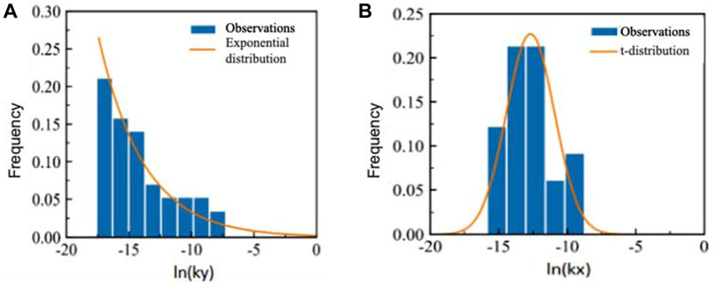
Figure 5. Characteristics of frequency distribution of soil hydraulic conductivity in (A) vertical and (B) horizontal directions.

Figure 6

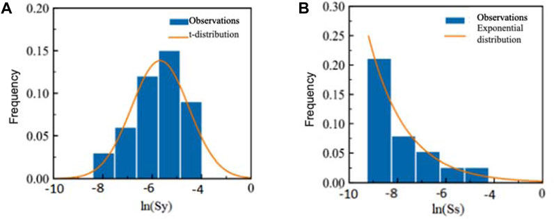
Figure 6. Characteristics of frequency distribution of soil (A) specific yield and (B) specific storage.

Table 1 presents the characteristic parameter values of the probability distribution function for various soil permeability coefficients. The KS test indicates a high degree of fitting for the distribution function, underscoring the evident distribution characteristics of relevant parameters in each soil layer.

Table 1

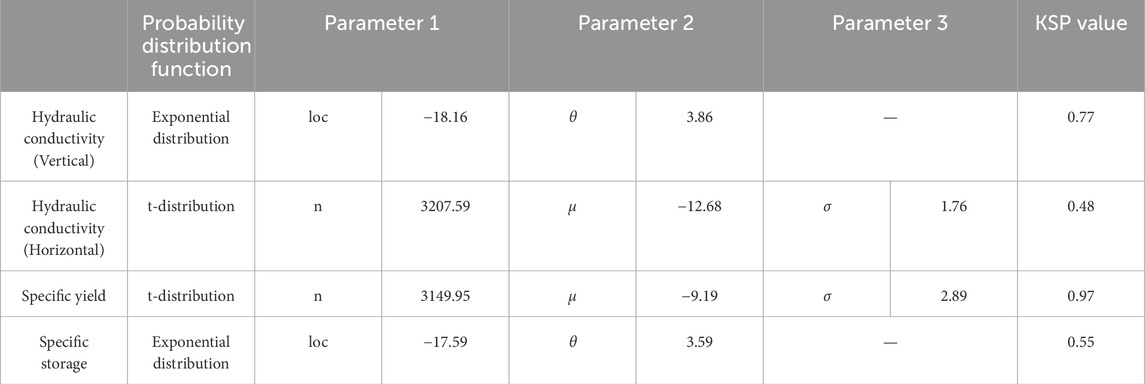
Table 1. Probability distribution function fitting parameters.

The essential parameters for this numerical simulation encompass aquifer permeability coefficient, specific yield, and water storage coefficient. Based on the test outcomes, probability distribution statistics of these parameters are conducted across distinct soil layers, yielding probability distribution curves for hydraulic conductivity, specific yield, and specific storage in each layer. Additionally, the median and confidence interval (at a 95% confidence level) of these parameters are calculated, as illustrated in Table 2.

Table 2

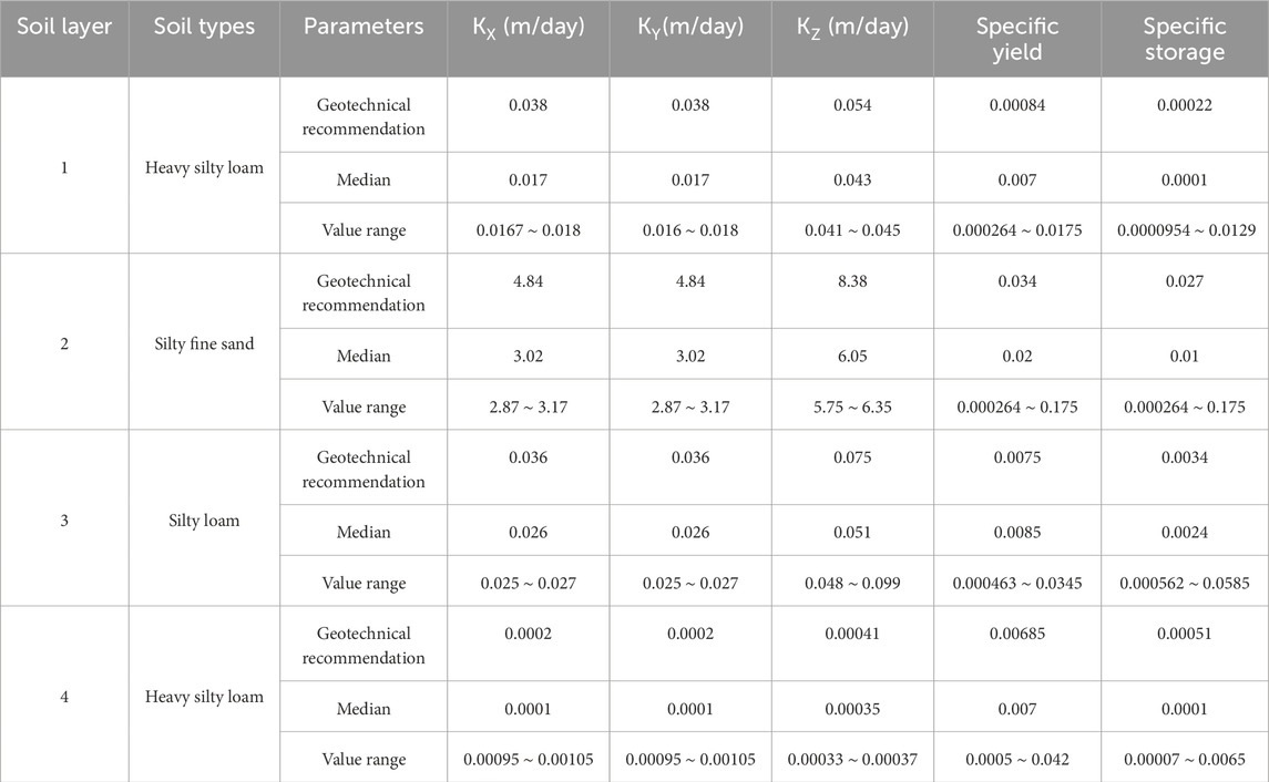
Table 2. Statistical table of hydrogeological parameters of each soil layer.

3.1.2 Source and sink

The dynamics of groundwater within the model are primarily influenced by the input of source and sink terms, comprising three elements within the simulation area: point, line, and surface. Point elements encompass sources and sinks such as agricultural exploitation. Linear elements predominantly denote recharge items from rivers (processed by the river module). Surface elements, provided by the Recharge module, primarily represent recharge items such as rainfall infiltration and irrigation infiltration. Data pertaining to other source and sink items, such as submersible evaporation, are incorporated into the model for computation through the Well module, all of which are processed into production or recharge wells.

3.1.3 Initial water head

Given the small area of the simulation zone and the simplicity of its hydrogeological conditions, in this study, we initially used the 2022 rainfall and river level data as drivers, with the ground elevation as the initial hydraulic head, to simulate the distribution of hydraulic heads under steady flow conditions. This simulated distribution was then used as the initial hydraulic head condition for subsequent simulation studies.

3.2 Numerical model

In accordance with the hydrogeological conceptual model, hydrogeological parameters and other boundary conditions are input into the model. Utilizing the parameter partition and value method outlined by the RFT model of soil parameters, and considering the hydrogeological conditions and characteristics of source-sink terms within the simulation area, the numerical model was solved using initial and boundary conditions. The numerical model of the groundwater flow field in the study area is illustrated in Figure 7.

Figure 7

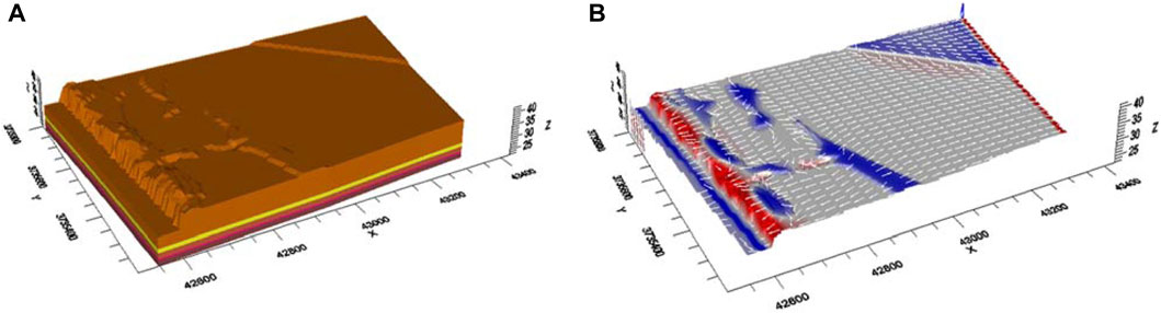
Figure 7. Three-dimensional structural map of the aquifer (A) and groundwater flow field simulation results (B).

4 Results

4.1 Model validation

To analyze whether the multi-parameter probability distribution model offers advantages in constructing the groundwater model, two sets of groundwater numerical simulation experiments were established. Under the same conditions of model boundaries, source-sink terms, time step, and so on, Model I serves as the control group, with hydrogeological parameters adopting the recommended values from geological surveys. Model II is the experimental group, with hydrogeological parameters using the median values obtained from the RFT as the initial model parameters. The parameter inversion range is determined by the confidence interval (confidence level of 95%). The model parameters are calibrated using the PEST module embedded in MODFLOW, and the final parameter values are determined.

The simulation period, spanning from 24 August 2022, to 24 February 2023, was designated as the calibration period, while the period from 24 February 2023, to 24 April 2023, was set as the validation period. The simulation results of Model I and Model II were compared with the corresponding measured groundwater levels, and the results are shown in Figure 8.

Figure 8

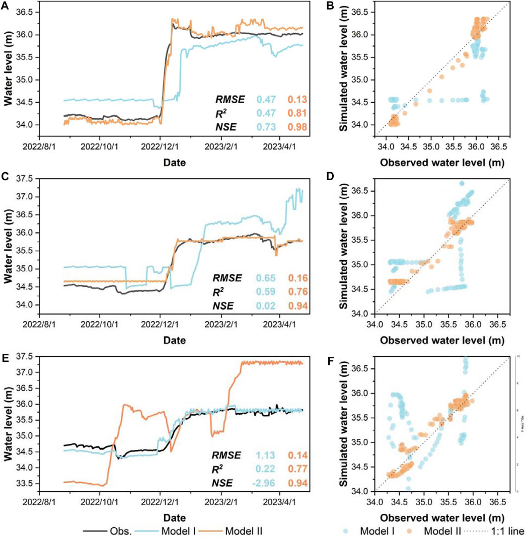
Figure 8. Measured and simulated groundwater level dynamics and their comparison in three observation wells, i.e., (A,B): Qsh 5–1, (C,D): Qsh 5–2, (E,F): Qsh 5-3.

In Model I, the RMSE values between the calculated water levels and the observations at Qsh 5-1, Qsh 5-2, and Qsh 5-3 are 0.47 m, 0.65 m, and 1.13 m, respectively. The corresponding R² values are 0.47, 0.59, and 0.22, while the NSE values are 0.73, 0.02, and −2.96, respectively. Conversely, in Model II, the RMSE values for the same observation points are notably lower, at 0.13 m, 0.16 m, and 0.14 m, respectively. Correspondingly, the R² values are significantly higher, measuring 0.81, 0.76, and 0.77, and the NSE values show considerable improvement, registering at 0.98, 0.94, and 0.94, respectively.

When comparing the simulated water levels with the observed ones, it becomes evident that in Model I, the maximum deviation between the calculated and observed water levels occurs at Qsh 5-3 on 24 October 2022, with a discrepancy of 127 cm. Conversely, the minimum deviation emerges at Qsh 5-3 on 24 January 2023, with a difference of 69 cm. In Model II, the maximum discrepancy between the calculated and observed water levels is also observed at Qsh 5-3 on 24 October 2022, albeit reduced significantly to 27 cm, representing a reduction of 78.7%. The smallest discrepancy, on the other hand, is noted at Qsh 5-2 on 24 December 2022, amounting to a mere 0.9 cm, showcasing a reduction of 98.7%.

Hence, the numerical model’s calculations, considering the multi-parameter random distribution, exhibit closer proximity to the actual observations, resulting in an enhanced model fitting degree.

4.2 Model parameter sensitivity analysis

To analyze the impact of hydrogeological parameter deviations on the simulated results, we constructed models using the values corresponding to the 5th, 50th, and 95th percentiles of the probability density function for hydraulic conductivity of each aquifer. We simulated river seepage under different parameter combinations. The results indicate that under normal river dispatch conditions, the maximum annual seepage on one side of the river during the operational period is 5.72×10⁵ m³, while the minimum seepage is 2.52×10⁵ m³, representing a variability of 126.9% relative to the minimum seepage. This demonstrates that the randomness of aquifer permeability significantly influences seepage rates.

4.3 Observation-based characterization of the response of groundwater to riverine water delivery

According to the actual measurement data of the groundwater level in the riverbank zone (Qsh5-1, Qsh5-2, Qsh5-3, Figure 2), after the initial experimental water transfer of the YHWDP from November 15 to 30, 2022, the dynamic response of the groundwater in the monitoring cross-section was significant. For instance, at monitoring point Qsh5-1, located about 50 m from the river channel, the water level was first recorded on 2 December 2022, rising from 34.39 m and reaching a peak of 36.16 m on 18 December 2022, taking a total of 6 days to rise 1.77 m. At Qsh5-2, about 100 m from the river channel, the water level was recorded beginning to rise from 34.55 m on 5 December 2022, and reached its highest at 35.67 m on 5 January 2023, taking a total of 31 days to rise 1.12 m. At Qsh5-3, approximately 150 m from the river channel, the water level started to rise from 34.65 m on 9 December 2022, and reached its peak at 35.71 m on 19 February 2023, taking a total of 72 days to rise 1.01 m.

Figure 9 shows the dynamics of the water levels, indicating that before the river water was transferred, the natural groundwater flow was replenishing the river, meaning the groundwater discharged into the river as baseflow. After the water transfer, the groundwater flow field reversed, with the river leaking water to replenish the groundwater. Additionally, due to varying distances between the monitoring points and the river channel, there were significant differences in groundwater changes, and a certain lag was present in the river replenishing the groundwater. For example, the rate of rise at Qsh5-1 and Qsh5-3 was 0.295 m/day and 0.015 m/day respectively, indicating that groundwater closer to the river channel was more significantly affected by the replenishment than that further away.

Figure 9

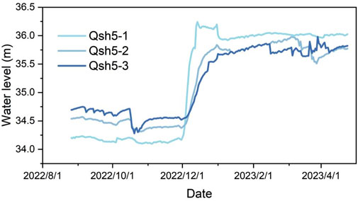
Figure 9. The groundwater dynamics in the observation wells.

4.4 Model-based effects of different river stages on groundwater flow fields

Based on the calibrated groundwater numerical model, while keeping other simulation conditions unchanged, the variations in the groundwater flow field under different river water levels, i.e., 34.5 m, 35.0 m, 35.5 m, 36.0 m, 36.5 m, and 37.0 m, were simulated. Taking the 80th day of the simulation period as an example, the average groundwater level heights along the direction perpendicular to the river are shown in Figure 10.

Figure 10

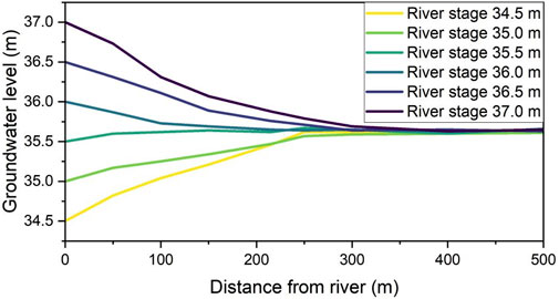
Figure 10. Simulated groundwater levels in the vertical channel direction for different river stages.

When the river water level is below 35 m, groundwater discharges into the river; when the river water level is above 35 m, the river recharges the groundwater. The strong interaction zone between the river and groundwater is approximately within 250 m from the river, and this distance slightly increases with the growing hydraulic gradient between the river and groundwater. As shown in the figure, when the river level is between 35.5 m and 36 m, the influence of the river on groundwater is minimal, with groundwater levels stabilizing around 100 m; when the river level is between 36.5 m and 37 m, the river recharges groundwater and its influence reaches the farthest, with groundwater levels stabilizing between approximately 250 m and 400 m.

4.5 Effects of farmland irrigation on river-groundwater exchange

Considering that the main land use type in the study area is farmland, and agricultural irrigation is an important discharge route for groundwater, it is crucial to explore whether different irrigation scenarios could have significant impacts on the surrounding groundwater flow field. For this purpose, we set up scenarios for both single-well and multi-well pumping, simulating a pumping period from September 15 to 19 September 2022, lasting 4 days, with a pumping rate of 400 cubic meters per hour and 8 h of pumping each day. The arrangement of the pumping wells is shown in Figure 2, where in the single-well scenario, water is pumped only from well1, and in the multi-well scenario, water is simultaneously pumped from wells well1, well2, and well3.

The results of the single-well and multi-well pumping simulations indicate that during the pumping period, the water levels near the pumping wells are significantly affected, resulting in the formation of a groundwater drawdown funnel. In the single-well scenario, the groundwater level changes around the well range from 5 to 8 m, and the area affected by the groundwater funnel ranges from 20 to 25 m. During this period, the farmland’s groundwater will be replenished by the river, with minimal impact. In the multi-well scenario, the groundwater level changes around the wells range from 12 to 17 m, and the area affected by the groundwater funnel ranges from 35 to 45 m. During this period, the farmland’s groundwater will be more significantly replenished by the river, resulting in a greater impact.

5 Discussion

5.1 The necessity of considering parameter stochasticity for groundwater modeling

The hydraulic head gradient between rivers and aquifers drives the dynamic changes in groundwater flow fields, and the rationality of hydrogeological parameters is one of the key factors determining the accuracy of groundwater numerical models. Due to the complexity of geological structures and tectonic origins, various geomorphic units and hydrogeological parameters of different scales exhibit significant spatial heterogeneity and display stochastic distribution characteristics. Although stochastic hydrology has been widely used in the study of surface hydrological processes, it is still to be deeply explored in groundwater theory (Tang et al., 2017).

First and foremost, the incorporation of parameter stochasticity enhances the realism and complexity of simulation. Comparing the groundwater numerical model based on multi-parameter probability distributions with the conventional model using geophysical recommendations for parameters, we found that the maximum deviation in simulated water levels decreased by 78.7%, the minimum deviation decreased by 98.7%, and the overall standard deviation decreased by 0.20 m. These results demonstrate that considering parameter distribution characteristics can significantly improve model parameter calibration efficiency and enhance the accuracy of groundwater numerical simulations.

Moreover, parameter stochasticity significantly impacts the interpretation of simulation results. The presence of random parameters often leads to variability and uncertainty in the outcomes. This requires us to not only focus on the average or trend of the results but also fully consider their variability and uncertainty. Additionally, we need to conduct sensitivity analysis of random parameters to understand their impact on simulation results, thereby enabling a more accurate interpretation.

Finally, parameter stochasticity also plays a crucial role in guiding the application of simulation results. When applying simulation outcomes to practical problems, we need to select appropriate settings for parameter stochasticity based on the specific situation and requirements of the problem. For instance, in some cases, we may need to increase the variability of random parameters to better mimic the complexity of systems; in others, we may want to reduce the variability to improve the stability and reliability of simulation results. Furthermore, we must develop corresponding strategies to address potential risks and challenges based on the uncertainty of simulation outcomes.

This paper focuses solely on the distribution frequency of model parameters. To more reasonably characterize the complex hydrogeological phenomena in the study area and accurately depict the spatial and temporal distribution and movement patterns of groundwater, it is necessary to conduct an in-depth analysis considering the spatially distributed random characteristics of parameters. Moreover, due to the small scope of the simulation area and the relatively simple geological conditions, we primarily conducted our analysis from the perspective of vertical randomness in stratigraphic parameters. Although we have found that the randomness of hydrogeological parameters of the aquifer has a significant impact on the intensity of interaction between rivers and groundwater, how this impact will change (increase or decrease) with the expansion of the research scale and the increase in stratigraphic complexity still requires further examination and verification.

5.2 Influencing factors of interaction mechanism between river water and groundwater in hyporheic zone

Groundwater, as a natural reservoir, features relatively uniform spatial distribution and stable water volume, which are crucial for maintaining ecosystems and sustainable development in arid regions (Wang et al., 2021; Wang et al., 2022). However, intensified human activities have led to severe phenomena such as shrinking surface water bodies and groundwater overexploitation, resulting in imbalanced or decoupled surface-groundwater interactions and escalating water conflicts between society and the natural system (Wang, 2018). Especially with the exacerbation of drought in arid regions, maintaining reasonable ecological baseflow becomes a key issue in the research of ecological security and sustainability (de Graaf et al., 2019; Allan and Douville, 2024).

Rivers are one of the most intense and widespread sites of interaction between surface and groundwater in arid regions. Many studies have shown that anthropogenic extraction-induced groundwater level decline has led to a sharp reduction in runoff in most arid region rivers globally, and even to phenomena such as surface-groundwater decoupling and river drying (Döll et al., 2009; Döll et al., 2012; Jasechko and Perrone, 2021). In recent years, intermittent river decoupling processes and their influencing factors, as well as the infiltration patterns of river water from saturation to complete decoupling, have become hotspots in the study of surface-groundwater exchange (Wang, 2018).

The main influencing factors of the interaction mechanism between river water and groundwater in the hyporheic zone are reflected in hydrological characteristics, riverbed sediment structure characteristics, human activities, and underlying surface conditions. Our research found that the hyporheic zone groundwater system was affected to varying degrees before and after river flow events. Observational results show that changes in river flow levels affect the direction, rate, and distance of surface water-groundwater interactions, with the severity of interaction between river water and groundwater in the hyporheic zone depending on factors such as river flow levels, permeability and particle size of riverbed sediments, and characteristics of the riparian aquifer.

However, due to the dynamic nature of the hyporheic zone, although many traditional monitoring and sampling techniques have been used in hyporheic zone research, and many new technologies have been introduced, existing monitoring techniques still face challenges in meeting research needs. Difficulties include synchronizing monitoring frequencies with groundwater changes, achieving full coverage of monitoring areas in regions with large and rapid changes over short periods. In the future, research is still needed on how to observe the entire process of interaction between river water and groundwater in the hyporheic zone.

5.3 Insights for the water management strategies of the YHWDP

The YHWDP is a grand inter-basin water transfer project aimed at connecting the Yangtze and Huaihe river systems, with the primary goals of meeting the water supply needs of urban and rural areas, developing Yangtze-Huaihe navigation, and simultaneously considering irrigation and replenishment as well as improving the water ecological environment of Chaohu Lake and the Huaihe River. To address the diverse water demands of the regions along the route, the project has adopted a comprehensive water delivery solution that includes natural rivers, storage reservoirs, and water pipelines.

In the Qingshui River section, which is the focus of this study, the project has chosen natural river channels as the main method of water conveyance, allowing moderate seepage of river water into the ground to alleviate the pressure on groundwater from agricultural irrigation and prevent the risk of overexploitation of groundwater. However, while ensuring this ecological benefit, it is also essential to ensure the stable supply of water for downstream receiving areas, especially for urban and rural domestic use. Therefore, an accurate assessment of the water exchange between the river and groundwater in the Qingshui River section is crucial for the efficient operation and maximum benefit of the entire water conveyance project.

This study, through site-scale simulation analysis of the groundwater flow field, found that the exchange intensity between the river and groundwater is highly sensitive to the river’s hydrological conditions and the hydrogeological parameters of the aquifer. Therefore, when assessing the seepage loss of the water conveyance project, it is necessary to fully consider the spatial heterogeneity of the river and aquifer hydraulic conductivity. For sections of the river with more serious seepage, it is recommended to take appropriate anti-seepage measures to reduce unnecessary water loss. Additionally, based on the actual groundwater extraction conditions in the region, dynamic adjustments to river water levels can be made to achieve both protection of groundwater reserves and avoidance of excessive water waste, thereby ensuring that the water diversion project can maximize its social and ecological benefits.

6 Conclusion

Based on indoor and outdoor soil tests conducted along the Qingshui River, significant hydrogeological parameters such as permeability coefficient, specific yield, and water storage rate were analyzed, and their probability distribution functions were established. Subsequently, a groundwater numerical model based on multi-parameter probability distribution was developed, utilizing the median range and confidence interval (at a confidence level of 95%) of parameter values. This model was then compared to a conventional model employing recommended values from geological exploration. The comparison revealed substantial enhancements in simulation accuracy, with the maximum disparity in water levels at observation points reduced by 78.7%, the minimum disparity by 98.7%, and the standard deviation by 0.20. These improvements signify a significant stride towards high-precision groundwater management.

Upon comparing the model calculations with observations, it becomes evident that under consistent conditions, when the river water level ranges between 34.5 m and 37 m, the hyporheic zone within the study area undergoes a transition from groundwater recharging the river to the river recharging groundwater. Consequently, the mutual influence zone between groundwater and the river expands from approximately 100 m to about 400 m. When comparing the effects of single-well and multi-well irrigation modules, it is observed that the surrounding groundwater level’s influence range and the groundwater funnel area increase by approximately 125% and 75%, respectively. This emphasizes that different simulation scenarios involving river flow, riverbed permeability coefficient, and irrigation areas directly influence the intensity of water exchange between the river and groundwater, as well as the characteristics of groundwater seepage and storage. These variations significantly impact the crucial calculations related to water exchange between the river and groundwater, as well as the analysis of the surrounding groundwater ecological environment.

This study reveals the significant impact of the stochasticity of hydrogeological parameters on the uncertainty of groundwater models. Coupling stochastic hydrology theory with groundwater dynamics will facilitate the improvement of groundwater model efficiency and simulation accuracy.

Data availability statement

The raw data supporting the conclusions of this article will be made available by the authors, without undue reservation.

Author contributions

JWa: Conceptualization, Investigation, Writing–original draft, Writing–review and editing. TW: Conceptualization, Writing–original draft, Writing–review and editing, Supervision. SZ: Resources, Writing–review and editing. RS: Data curation, Formal Analysis, Software, Writing–original draft. YL: Data curation, Resources, Writing–review and editing. YZ: Data curation, Methodology, Software, Writing–review and editing. MD: Investigation, Writing–review and editing. TZ: Investigation, Resources, Writing–review and editing. JWu: Methodology, Visualization, Writing–review and editing. QZ: Data curation, Visualization, Writing–review and editing.

Funding

The author(s) declare that financial support was received for the research, authorship, and/or publication of this article. This work was supported by grants from the Fundamental scientific research business expenses special project of the Engineering Research Service Project of Yangtze-to-Huaihe River Diversion Project (Henan Section) (HN-YJJH/JS/FWKY-2021001), the Yellow River Institute of Water Conservancy Sciences (HKY-JBYW-2023-07) and the Open Project Fund of the Embankment Safety and Disease Control Engineering Technology Research Center of the Ministry of Water Resources (LSDP202402).

Conflict of interest

Author TZ was employed by Henan Yangtze-to-Huaihe Water Diversion Co., Ltd. Author QZ was employed by Henan Seventh Geological Brigade Co., Ltd.

The remaining authors declare that the research was conducted in the absence of any commercial or financial relationships that could be construed as a potential conflict of interest.

Publisher’s note

All claims expressed in this article are solely those of the authors and do not necessarily represent those of their affiliated organizations, or those of the publisher, the editors and the reviewers. Any product that may be evaluated in this article, or claim that may be made by its manufacturer, is not guaranteed or endorsed by the publisher.

References

Allan, R. P., and Douville, H. (2024). An even drier future for the arid lands. Proc. Natl. Acad. Sci. 121 (2), e2320840121. doi:10.1073/pnas.2320840121

PubMed Abstract | CrossRef Full Text | Google Scholar

Bonanno, E., Blöschl, G., and Klaus, J. (2021). Flow directions of stream-groundwater exchange in a headwater catchment during the hydrologic year. Hydrol. Process. 35 (8), e14310. doi:10.1002/hyp.14310

CrossRef Full Text | Google Scholar

Cao, G., Zheng, C., Scanlon, B. R., Liu, J., and Li, W. (2013). Use of flow modeling to assess sustainability of groundwater resources in the North China Plain. Water Resour. Res. 49 (1), 159–175. doi:10.1029/2012wr011899

CrossRef Full Text | Google Scholar

Cao, L., Nie, Z., Liu, M., Wang, L., Wang, J., and Wang, Q. (2021). The ecological relationship of groundwater–soil–vegetation in the oasis–desert transition zone of the shiyang River basin. Water 13 (12), 1642. doi:10.3390/w13121642

CrossRef Full Text | Google Scholar

Cho, S. E. (2012). Probabilistic analysis of seepage that considers the spatial variability of permeability for an embankment on soil foundation. Eng. Geol. 133-134, 30–39. doi:10.1016/j.enggeo.2012.02.013

CrossRef Full Text | Google Scholar

Cornell, C. A. (1972). “First-order uncertainty analysis of soil deformation and stability,” in International Conference on Applications of Statistics and Probability to Soil and structural engineering, 1st (Hong Kong: Hong Kong University Press), 130–143.

Google Scholar

de Graaf, I. E. M., Gleeson, T., van Beek, L. P. H., Sutanudjaja, E. H., and Bierkens, M. F. P. (2019). Environmental flow limits to global groundwater pumping. Nature 574 (7776), 90–94. doi:10.1038/s41586-019-1594-4

PubMed Abstract | CrossRef Full Text | Google Scholar

Döll, P., Fiedler, K., and Zhang, J. (2009). Global-scale analysis of river flow alterations due to water withdrawals and reservoirs. Hydrol. Earth Syst. Sci. 13 (12), 2413–2432. doi:10.5194/hess-13-2413-2009

CrossRef Full Text | Google Scholar

Döll, P., Hoffmann-Dobrev, H., Portmann, F. T., Siebert, S., Eicker, A., Rodell, M., et al. (2012). Impact of water withdrawals from groundwater and surface water on continental water storage variations. J. Geodyn. 59-60, 143–156. doi:10.1016/j.jog.2011.05.001

CrossRef Full Text | Google Scholar

Jasechko, S., and Perrone, D. (2021). Global groundwater wells at risk of running dry. Science 372 (6540), 418–421. doi:10.1126/science.abc2755

PubMed Abstract | CrossRef Full Text | Google Scholar

Ji, Z., Cui, Y., Zhang, S., Chao, W., and Shao, J. (2021). Evaluation of the impact of ecological water supplement on groundwater restoration based on numerical simulation: a case study in the section of yongding river, Beijing plain. Water 13 (21), 3059. doi:10.3390/w13213059

CrossRef Full Text | Google Scholar

Ji, W., Luo, Y., Liu, J., Li, X., Li, L., Yu, D., et al. (2023). Stochastic simulation of leaching range in in-situ leaching process considering uncertainty of permeability coefficient. Atomic Energy Sci. Technol. 57 (6), 1099. doi:10.7538/yzk.2022.youxian.0622

CrossRef Full Text | Google Scholar

Kumar, S., Dwivedi, A. K., Ojha, C. S. P., Kumar, V., Pant, A., Mishra, P. K., et al. (2022). Numerical groundwater modelling for studying surface water-groundwater interaction and impact of reduced draft on groundwater resources in central Ganga basin. Math. Biosci. Eng. 19 (11), 11114–11136. doi:10.3934/mbe.2022518

PubMed Abstract | CrossRef Full Text | Google Scholar

Lei, J., Xia, L., Wang, Q., Cao, X., and Chen, J. (2016). Random prediction model of geological section for non-homogeneous formation. Chin. J. Undergr. Space Eng. 12 (1), 84–89.

Google Scholar

Li, W., Lu, Z., and Zhang, D. (2009). Stochastic analysis of unsaturated flow with probabilistic collocation method. Water Resour. Res. 45 (8). doi:10.1029/2008wr007530

CrossRef Full Text | Google Scholar

Liu, F., Hu, X., Zhen, P., Zou, J., and Zhang, J. (2023). Characterizing groundwater recharge sources within reduced pumped aquifers in the Heilonggang region, North China Plain. J. Geochem. Explor. 247, 107176. doi:10.1016/j.gexplo.2023.107176

CrossRef Full Text | Google Scholar

Lumb, P. (1975). Spatial variability of soil properties proc., 2nd int. Conf. On Application of Statistics and Probability in Soil and structural engineering, 397–421.

Google Scholar

Lyu, K., Zhang, Q., Cui, Y., Zhang, Y., Zhou, Y., Lyu, L., et al. (2024). Optimizing recharge area delineation for small-to medium-sized groundwater systems through coupling methods and numerical modeling: a case study of linfen city, China. Sustainability 16 (4), 1465. doi:10.3390/su16041465

CrossRef Full Text | Google Scholar

Ni, L., Wang, W., Zhao, W., Qu, S., and Sun, X. (2021). Numerical simulation and regulation analysis of subsurface flow for an underground reservoir in Weihai. IOP Conf. Ser. Earth Environ. Sci. 621 (1), 012122. doi:10.1088/1755-1315/621/1/012122

CrossRef Full Text | Google Scholar

Prajapati, R., Overkamp, N. N., Moesker, N., Happee, K., van Bentem, R., Danegulu, A., et al. (2021). Streams, sewage, and shallow groundwater: stream-aquifer interactions in the Kathmandu Valley, Nepal. Sustain. Water Resour. Manag. 7 (5), 72. doi:10.1007/s40899-021-00542-8

CrossRef Full Text | Google Scholar

Ramadas, M., Ojha, R., and Govindaraju, R. S. (2015). Current and future challenges in groundwater. II: water quality modeling. J. Hydrologic Eng. 20 (1), A4014008. doi:10.1061/(asce)he.1943-5584.0000936

CrossRef Full Text | Google Scholar

Rezapour, T. M. M., and Yazdi, A. (2014). Conjunctive use of surface and groundwater with inter-basin transfer approach: case study piranshahr. Water Resour. Manag. 28 (7), 1887–1906. doi:10.1007/s11269-014-0578-2

CrossRef Full Text | Google Scholar

Santoso, A. M., Phoon, K.-K., and Quek, S.-T. (2011). Effects of soil spatial variability on rainfall-induced landslides. Comput. Struct. 89 (11), 893–900. doi:10.1016/j.compstruc.2011.02.016

CrossRef Full Text | Google Scholar

Schiavo, M. (2024). Numerical impact of variable volumes of Monte Carlo simulations of heterogeneous conductivity fields in groundwater flow models. J. Hydrology 634, 131072. doi:10.1016/j.jhydrol.2024.131072

CrossRef Full Text | Google Scholar

Shu, L., Chen, H., Meng, X., Chang, Y., Hu, L., Wang, W., et al. (2024). A review of integrated surface-subsurface numerical hydrological models. Sci. China Earth Sci. 67 (5), 1459–1479. doi:10.1007/s11430-022-1312-7

CrossRef Full Text | Google Scholar

Srivastava, A., Babu, G. L. S., and Haldar, S. (2010). Influence of spatial variability of permeability property on steady state seepage flow and slope stability analysis. Eng. Geol. 110 (3), 93–101. doi:10.1016/j.enggeo.2009.11.006

CrossRef Full Text | Google Scholar

Tang, Q., Kurtz, W., Schilling, O. S., Brunner, P., Vereecken, H., and Hendricks Franssen, H. J. (2017). The influence of riverbed heterogeneity patterns on river-aquifer exchange fluxes under different connection regimes. J. Hydrology 554, 383–396. doi:10.1016/j.jhydrol.2017.09.031

CrossRef Full Text | Google Scholar

Vanmarcke, E. H. (1977). Probabilistic modeling of soil profiles. J. Geotechnical Eng. Div. 103 (11), 1227–1246. doi:10.1061/ajgeb6.0000517

CrossRef Full Text | Google Scholar

Wang, P. (2018). Progress and prospect of research on water exchange between intermittent rivers and aquifers in arid regions of northwestern China. Prog. Geogr. 37 (2), 183–197. doi:10.18306/dlkxjz.2018.02.002

CrossRef Full Text | Google Scholar

Wang, T., Wang, P., Wu, Z., Yu, J., Pozdniakov, S. P., Guan, X., et al. (2022). Modeling revealed the effect of root dynamics on the water adaptability of phreatophytes. Agric. For. Meteorology 320, 108959. doi:10.1016/j.agrformet.2022.108959

CrossRef Full Text | Google Scholar

Wang, T., Wu, Z., Wang, P., Wu, T., Zhang, Y., Yin, J., et al. (2023). Plant-groundwater interactions in drylands: a review of current research and future perspectives. Agric. For. Meteorology 341, 109636. doi:10.1016/j.agrformet.2023.109636

CrossRef Full Text | Google Scholar

Wang, T.-Y., Wang, P., Wang, Z.-L., Niu, G.-Y., Yu, J.-J., Ma, N., et al. (2021). Drought adaptability of phreatophytes: insight from vertical root distribution in drylands of China. J. Plant Ecol. 14 (6), 1128–1142. doi:10.1093/jpe/rtab059

CrossRef Full Text | Google Scholar

Wu, T. H. (1974). Uncertainty, safety, and decision in soil engineering. J. Geotechnical Eng. Div. 100 (3), 329–348. doi:10.1061/ajgeb6.0000026

CrossRef Full Text | Google Scholar

Ya, L. (2019). Study on rainfall failure probability of slope with weak interlayer considering spatial variability of soil parameters. Water Resour. Power 37 (12), 103–107.

Google Scholar

Yang, Z., Hu, L., and Sun, K. (2021). The potential impacts of a water transfer project on the groundwater system in the Sugan Lake Basin of China. Hydrogeology J. 29 (4), 1485–1499. doi:10.1007/s10040-021-02337-9

CrossRef Full Text | Google Scholar

Yuan, R., Wang, M., Wang, S., and Song, X. (2020). Water transfer imposes hydrochemical impacts on groundwater by altering the interaction of groundwater and surface water. J. Hydrology 583, 124617. doi:10.1016/j.jhydrol.2020.124617

CrossRef Full Text | Google Scholar

Zhang, J., Liu, T., Dong, J., Wang, X., Zha, Y., Tang, X., et al. (2020). The impact of aquifer layered heterogeneity on groundwater flow system. Geol. CHINA 47 (6), 1715–1725. doi:10.12029/gc20200609

CrossRef Full Text | Google Scholar

Zhao, M., Meng, X., Wang, B., Zhang, D., Zhao, Y., and Li, R. (2022). Groundwater recharge modeling under water diversion engineering: a case study in beijing. Water 14 (6), 985. doi:10.3390/w14060985

CrossRef Full Text | Google Scholar

Zhao, T., Richards, K. S., Xu, H., and Meng, H. (2012). Interactions between dam-regulated river flow and riparian groundwater: a case study from the Yellow River, China. Hydrol. Process. 26 (10), 1552–1560. doi:10.1002/hyp.8260

CrossRef Full Text | Google Scholar

Zhu, H., Zhang, L. M., Zhang, L. L., and Zhou, C. B. (2013). Two-dimensional probabilistic infiltration analysis with a spatially varying permeability function. Comput. Geotechnics 48, 249–259. doi:10.1016/j.compgeo.2012.07.010

CrossRef Full Text | Google Scholar

Zhu, M., Wang, S., Kong, X., Zheng, W., Feng, W., Zhang, X., et al. (2019). Interaction of surface water and groundwater influenced by groundwater over-extraction, waste water discharge and water transfer in xiong’an new area, China. Water 11 (3), 539. doi:10.3390/w11030539

CrossRef Full Text | Google Scholar