 Yu Lei
 Li Jianyong3*
 Ji Wei
 Ma Weiyu
94% of researchers rate our articles as excellent or good
Learn more about the work of our research integrity team to safeguard the quality of each article we publish.
Find out more
METHODS article
Front. Earth Sci., 13 September 2024
Sec. Solid Earth Geophysics
Volume 12 - 2024 | https://doi.org/10.3389/feart.2024.1423823
This article is part of the Research TopicFaults and Earthquakes Viewed by Networks, Monitoring Systems and by Numerical Modelling TechniquesView all 11 articles
Since 1966, China has been using apparent resistivity observation to forecast strong aftershocks of the Xingtai earthquake. Retrospective studies of subsequent strong earthquakes have shown that anomalies in apparent resistivity observation before earthquakes usually exhibit anisotropic characteristics. In addition to the anisotropic changes in apparent resistivity before earthquakes, factors such as subway operation near the observation area, metal pipeline networks, and changes in water levels have also been found to cause anisotropic changes. These factors are called environmental interference factors. Therefore, distinguishing between anisotropic changes before earthquakes and anisotropic changes caused by interference and eliminating the effects of interference is crucial for using apparent resistivity observations for forecasting. Taking the observation of Hefei seismic station in Anhui Province as an example, a model is constructed using the finite element method to try to establish a method for analyzing anisotropy in apparent resistivity before earthquakes, and the data from other provincial stations are used for verification. In the modeling process, the influence coefficient is a measure of the relationship between the variation in apparent resistivity and the changes in the medium of the measurement area. The following results are obtained by calculating the influence coefficient using the finite element method: the influence coefficient between the power supply electrode and the measuring electrode of the apparent resistivity observation is negative, and the rest are positive, and the distribution of the influence coefficient shows obvious symmetry, with the axis of symmetry being the line connecting the electrodes and its midline, and the absolute value of the influence coefficient is inversely proportional to the distance from the electrodes. In addition, according to the constructed finite element model, the amplitude of anisotropic changes caused by interference can be quantitatively calculated. Given that interference is ubiquitous in various regions of the world, this study can provide a reference for international earthquake forecasters to quantitatively remove environmental interference in anisotropy. Moreover, when building apparent resistivity stations in seismic areas for earthquake prediction, it is best to avoid areas with larger local influence coefficients to ensure that the anomalous data before the earthquake is true and reliable.
The seismic method of apparent resistivity in seismology is employed to predict earthquakes by monitoring temporal variations in the electrical properties of the Earth’s media. After the 1966 Xingtai earthquake, China initiated the use of apparent resistivity methods to forecast strong aftershocks of the earthquake. Subsequent retrospective studies on several major earthquakes have shown that anomalies in apparent resistivity observation before the earthquakes typically exhibit characteristics of anisotropy. Over the past 50 years, this network has grown to encompass over 90 stations. During the operation of the seismic network, the theory of anisotropic variations has evolved and played a role in earthquake monitoring and forecasting (Zhao et al., 1983; Ellis et al., 2010; Bachrach, 2011; North and Best, 2014; Sævik et al., 2014; Thongyoy et al., 2023). Moreover, observations of apparent resistivity changes have been utilized to predict certain moderate earthquakes (Du, 2010; Xu et al., 2014).
With ongoing societal development, various observation sites now confront varying degrees of interference. During the operation of subways, the presence of metal pipeline networks, and changes in water levels can cause local variations in the medium of the measurement area, thereby affecting the electrical structure of the area and resulting in anisotropic changes in the observation. However, these changes are not the pre-seismic anisotropic anomalies required for earthquake prediction. During routine observations, initial cracks in the medium may close or shift under increasing stress. Eventually, new cracks tend to form along the direction of maximum principal stress (Kemeny, 1991). To analyze the relationship between the apparent resistivity changes and variations in the geological medium, global geoelectric researchers have developed theories focusing on one-dimensional sensitivity coefficients for layered media. According to this theory, the relative change in apparent resistivity can be expressed as a weighted sum of relative changes across different regions of the observation area (Qian et al., 1985; Qian et al., 1996; Qian et al., 2013; Park and Van, 1991). This approach has been particularly useful in analyzing disturbances caused by changes in shallow subsurface materials (Lu et al., 1999; Lu et al., 2004). However, challenges arise at many stations where disturbances do not result from uniform changes in a single layer but rather from factors affecting multiple layers near electrodes, such as road construction and excavation. These multi-layer disturbances can complicate the application of traditional one-dimensional sensitivity coefficient theories, necessitating more sophisticated modeling techniques to accurately interpret observed data. Experts have employed a series of 40 theoretical horizontal resistivity profiles to investigate these phenomena. These profiles illustrate how factors like sinkhole dimensions, reflection coefficients (k), and lateral distance from the sinkhole center influence apparent resistivity observation (Kenneth and Russell, 1961). Researchers have observed variations in sensitivity coefficients across different regions of observation areas based on this theoretical framework (Xie and Lu, 2015). While these studies offer qualitative analyses of anomalous apparent resistivity changes, refining quantitative modeling methods remains an ongoing endeavor.
This study utilizes observational data from the Hefei seismic station in Anhui Province to explore the anisotropic variations in apparent resistivity measurements. Building on these findings, a three-dimensional influence coefficient model is constructed using the finite element method to quantitatively exclude the data variation amplitude caused by environmental interference in anisotropic changes. The developed method is then validated at the Xingji seismic station in Hebei Province, with the aim of establishing a method for determining the genuine pre-seismic apparent resistivity anisotropy. This research is intended to provide a reference for the apparent resistivity forecasting and station construction efforts in other seismically active regions internationally.
In shallow layers of the Earth’s surface, two principal stresses typically align horizontally. Under prolonged tectonic stress, the distribution and expansion of microcrack systems are controlled by the maximum principal stress (Crampin et al., 1984). For a uniform medium, when using a symmetric quadrupole array for surface observations, the apparent resistivity is given by (Kraev, 1954; Qian et al., 1996) and can be represented as Equation 1.
In the Formula
After a microcrack system expands along the
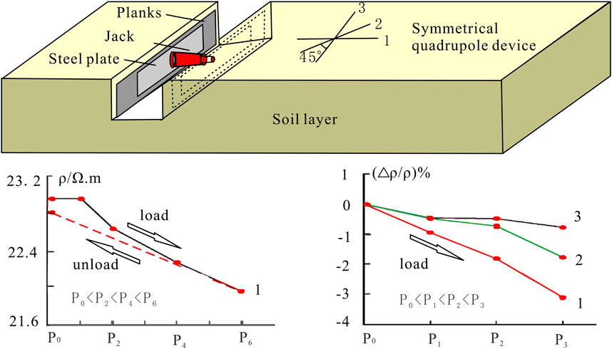
Figure 1. Anisotropic apparent resistivity variations in grooved soil under compressive stress (Zhao et al., 1983).
Subsurface formations often display lateral heterogeneity, which can cause apparent resistivity values to vary across different directions. However, according to finite element numerical analysis, the effect of lateral heterogeneity on anisotropic changes, quantified by the relative change ratio
Earthquakes result from long-term accumulation of tectonic stresses, eventually leading to fault instability. Anomalies in apparent resistivity typically occur 1–2 years before major earthquakes. During this period, the subsurface medium undergoes initial closure and deviation of cracks due to prolonged stress accumulation, eventually entering a phase dominated by a new crack system (Crampin et al., 1984). The magnitude of apparent resistivity anomalies varies in different directions relative to the principal stress axis: the greater the angle with the principal stress axis, the greater the anomaly magnitude. Significant anomalies were observed at stations such as Chengdu, Jiangyou, Ganzi, and Wudu before the 2008 Wenchuan Ms8.0 earthquake (Du et al., 2017; Zhang et al., 2009; Qian et al., 2013). However, there are differences in the magnitude of data changes among different directional measurements. Table 1 provides information on the apparent resistivity anomaly changes in different directions at various stations before the 2008 Wenchuan earthquake. These stations are located at varying distances from the epicenter, ranging from 30 to 330 km. The duration and magnitude of anomalies in different measurement directions before the earthquake also show significant differences, exhibiting a clear anisotropy.
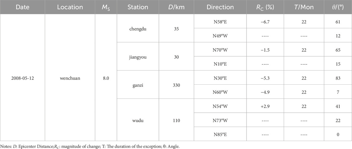
Table 1. The apparent resistivity changes before the 2008 Wenchuan earthquakes.
Apparent resistivity data exhibiting a downward trend that breaks the annual variation is a significant indicator of anomaly. The magnitude of anomalies often varies across different measurement directions, which is called pre-seismic anisotropy. For example, before the Ms8.0 Wenchuan earthquake in 2008, the N70°W measurement direction at the Jiangyou station, which is 30 km away from the epicenter, began to show a downward change in August 2006, with a decrease of about 1.5%. The N10°E measurement direction showed no significant changes before the earthquake. On the day of the earthquake, the N70°W and N10°E measurement directions decreased by 3.8% and 5.2% respectively. Post-earthquake, the data recovered and rose (Figures 2A, B).
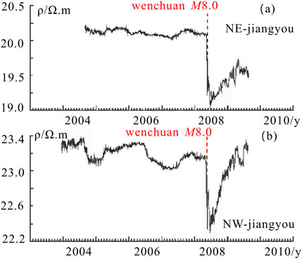
Figure 2. Typical trend of apparent resistivity before earthquake. (A) The change of N10°E direction data and (B) The change of N70°W direction data in Jiangyou station.
According to the theory of anisotropy, it’s feasible to identify and explain certain pre-seismic anomalous changes. However, contemporary apparent resistivity observations are susceptible to diverse influences, rendering the reasons quite intricate. Some anomalous changes may stem from local environmental alterations. If non-seismic anomalies cannot be accurately discerned, the efficacy of apparent resistivity observations could be compromised. Therefore, effectively identifying various disturbances forms the cornerstone for conducting anisotropy analysis.
Hefei seismic station is located in Hefei, Anhui Province, situated in a hilly area with micro-topography. The Tanlu Fault Zone traverses the station. The active faults within the Tanlu fault zone in Anhui are predominantly located at the boundary of the faulted basin, extending from south to north along the eastern boundary of the Hefei Basin, the eastern boundary of the Dabie Mountains orogenic belt, and the eastern and western boundaries of the Jiashan Basin (Ni et al., 2022). The epicenters of the 1,673 Hefei M5 earthquake and the 1,585 Chaohu M53/4 earthquake were in close proximity to the station.
The apparent resistivity measurement area is located in Anhui province, featuring a gentle slope from east to west and no significant slope in the north-south direction. The measurement area includes some paddy fields and is free of building facilities and underground pipelines. Apparent resistivity observation is set up with two directions: north-south (NS) and east-west (EW), employing symmetrical four-electrode burial (Figure 3C). The electrode is a 1 m × 1.1 m lead plate, buried at a depth of 2.0 m, with a grounding resistance range of 2–5Ω. The outer circuit consists of single-core copper wire with a plastic skin, supported by overhead cement poles. The distance between the power supply electrodes AB and the measuring electrodes MN is 600 m and 200 m, respectively. When the Chinese fixed station is conducting apparent resistivity observation, the detection range in the depth direction is comparable to the observation electrode distance AB scale, mainly reflecting the changes in the resistivity of the shallow layer medium. The observation electrode distance AB of Hefei station is 600 m, so the apparent resistivity observed by Hefei station is a comprehensive reflection of the medium resistivity from the surface to a depth of 600 m underground.
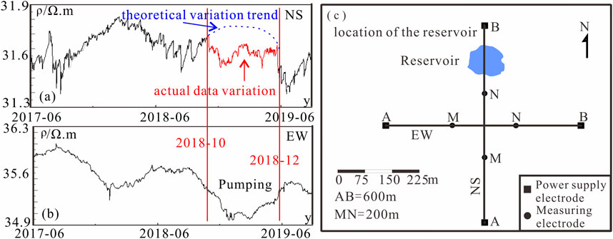
Figure 3. The change of apparent resistivity before and after pumping and the position of the reservoir. (A,B) the curve between the vertical lines show the changes after pumping water. (C) The position of the reservoir.
Based on the distribution of influence coefficients and multi-year observational data, the two directional apparent resistivity observation at the Hefei station have long shown an inverse variation over the years. However, between October 2018 and December 2018, the observation in both directions exhibited a synchronous change, which is a clear anisotropic variation (Figures 3A, B). In Figure 3A, the theoretical observation trend for the NS direction and the actual change curve form an inverse variation, and by comparing with Figure 3B, the change in the NS direction observation while the EW direction remains unchanged, causes the actual curves of the two directions to change from inverse to the same direction, resulting in anisotropic variation. Upon investigating the anomaly, it was found that there is a natural reservoir located between electrode positions B and N in the NS direction of the apparent resistivity observation setup at the station (Figure 3C). This reservoir maintains a stable water level throughout the year. In October 2018, the water level in the reservoir decreased significantly, leading to a reduction in the moisture content in the medium between positions B and N. According to the apparent resistivity calculation formula, a decrease in moisture content should result in an increase in apparent resistivity. However, the observed data showed a decrease instead (Figure 3B). This anomalous decrease in the NS data caused the previously opposite trends in NS and EW data curves to become synchronous starting from October 2018. During this period, there was an anisotropic change observed in the NS and EW data.
It is crucial to conduct a detailed analysis to determine the cause of this change. The anomaly could potentially be attributed to seismic precursor variations caused by anisotropy or environmental disturbances, such as changes in moisture content due to the fluctuating water level in the reservoir. Further investigation and monitoring will be necessary to understand the exact nature of these anomalous changes in apparent resistivity observation at Hefei station.
The apparent resistivity of the station in China uses a steady flow source for power supply, and is observed once every hour. One observation collects 10 sets of data, and then the average value is calculated, with the standard deviation of the observation controlled within 1%. Each quarter, the instrument is calibrated with a standard power source and standard resistance to ensure the accuracy of the observed values. The influence coefficient is used to analyze the extent of the impact that the resistivity changes of different positions in the measurement area may have on the observation.
Park and Van (1991) proposed that the influence coefficient is a measure of the relationship between the changes in apparent resistivity and the variations in the medium of the measurement area. When the electrical structure of the measurement area is determined and the observation system is stable, the apparent resistivity can be expressed as a function of the resistivity of the medium in each sub-zone (Lu et al., 2004):
Since the higher-order terms beyond the first are typically negligible, Equation 3 is a Taylor series approximation that omits second-order and higher terms. Consequently, the relative change in apparent resistivity can be articulated as a weighted sum of the relative changes in resistivity of each layer and it can be represented as Equation 4.
Based on the layered horizontal structure of the apparent resistivity measurement area, the influence coefficients B for a symmetric quadrupole arrangement can be calculated using the potential distribution analytical expression and the resistivity filter algorithm (O’Neill and Merrick, 1984; Yao, 1989). The coefficient B is defined as:
The one-dimensional influence coefficient is for horizontally layered stratification, treating each layer as a whole and analyzing the impact of changes in this whole on apparent resistivity observations. It is suitable for situations that can be equivalently transformed into changes of a whole layer, such as rainfall, temperature, and water level variations. However, the one-dimensional influence coefficient cannot be used to analyze the impact of localized changes in the medium on observations. Therefore, numerical simulation methods are needed to further subdivide the one-dimensional influence coefficients into three-dimensional influence coefficients.
Calculating three-dimensional influence coefficients requires the use of numerical simulation methods. There are many numerical simulation methods currently available, such as the finite element method, finite difference method, boundary element method, and other techniques. These methods for computing steady-state electrical current fields are now highly developed. Finite element methods are particularly adept at discretizing irregular geometries effectively. Considering the irregularly shaped reservoir within the observation area at Hefei Station, the finite element method for steady-state electrical current fields proves suitable for accurately modeling the station’s observation conditions.
When employing the Wenner array for observation, the measured apparent resistivity provides a comprehensive reflection of the subsurface resistivity over a defined volume of the measurement area. As the distance from the observation site increases, the impact of the medium on the observed values diminishes. At sufficiently large distances, this influence becomes negligible (Li, 2005). Given an electrode spacing of AB = 600 m for apparent resistivity observations, significant influences on the observations are confined to specific depths within the subsurface. Longitudinally, the site is stratified based on the electrical structure of the area, with the deepest layer extending up to twice the length of AB. Laterally, it extends to six times the length of AB. The three-dimensional influence coefficients of the surrounding medium at the observation site are analyzed using finite element numerical analysis methods.
Currently, apparent resistivity observations are conducted using a steady current source with a supply intensity typically ranging from 1 to 2 A. Therefore, the computation of apparent resistivity observations can be viewed as a steady-state electric current field problem, which can be expressed by Poisson’s Equation 7:
Where V is the potential generated by the current source I, σ is the dielectric conductivity, and δ (x, y, z) is the Dirac delta function. At the boundary of the model, steady current field satisfy Dirichlet-Neumann boundary condition and it can be represented as Equation 8.
The entire boundary of the finite medium space is Γ. A portion of the boundary has no current flow out (such as the ground surface), satisfying the Neumann boundary condition, denoted as ΓV. The remaining boundary is denoted as Γs, satisfying the Dirichlet boundary condition. Among them some parameters can be represented as Equations 9, 10.
n is the normal direction pointing outward from the boundary of the region The weak solution of Poisson equation of steady current field can be obtained by using the principle of virtual work.
Ω is the computational domain,
In apparent resistivity observations, the Earth’s surface naturally satisfies the Neumann boundary condition. At the infinite boundary, one can impose either Dirichlet boundary conditions (V = 0) or Neumann boundary conditions (Coggon, 1971). In practical applications, the model scale is finite by necessity. When the model size is fixed and the electrode spacing increases, computing apparent resistivity values with Dirichlet boundary conditions at infinity tends to underestimate the actual values, whereas using Neumann boundary conditions yields results that overestimate the actual values (Dey and Morrison, 1979; Li and Spitzer, 2005).
To minimize the boundary effects on computed results, one can enlarge the model size while keeping the electrode spacing fixed, although this approach increases computational complexity. Therefore, selecting an appropriate model size is crucial. Scholars have suggested, through finite element numerical analysis of apparent resistivity observations, that the horizontal dimension of the model should be greater than 6 times the electrode spacing (AB), and the model thickness should be greater than 2 times AB to effectively disregard boundary effects (Xie et al., 2014).
The site’s medium is subdivided into three-dimensional volumes of specific sizes, forming a model using the finite element numerical analysis method. After discretizing the elements and applying current sources and boundary conditions, numerical solutions are computed for the degrees of freedom (potentials) at the nodes of the elements. Using the solved potential differences, apparent resistivity values and corresponding distributions of influence coefficients are calculated based on device coefficients. The influence coefficient for a specific layer of the medium is determined by summing all influence coefficients from the three-dimensional volumes within that layer and it can be represented as Equation 12.
The specific parameters of the apparent resistivity observation instrument at the Hefei station site are as follows: the electrode spacing for the power supply electrodes AB is 600 m, and for the measuring electrodes MN it is 200 m. The observation device is positioned on the surface of the model, with the horizontal dimensions of the model set at 8 times AB. According to the electrical structure, the model is segmented into three layers, with the bottom layer having a thickness of 2 times AB. The calculation region for the influence coefficients spans around the center of the electrode array, covering a spatial extent of 4,800 m × 4,800 m × 1,200 m (Figure 4).
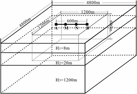
Figure 4. Schematic diagram of the finite element numerical analysis model. The model is divided into 3 layers, with the horizontal dimension taken as 8 times AB, and the thickness of the bottom layer taken as 2 times AB.
Given the fixed site conditions and the electrical structure described by Equation 2, each block within the site is independent in terms of its influence coefficients from other blocks. Therefore, this study uniformly divides the analysis region into several cubic units measuring 2 m × 2 m × 2 m. To optimize computational efficiency, the remaining areas gradually expand outward during unit division. During calculations, a current of 2I is applied to electrode A and -2I to electrode B. Each unit within the analysis region is computed using central differences to calculate the partial derivatives, as described in Equation 5. This process yields the respective influence coefficients for each unit, collectively forming the three-dimensional distribution of influence coefficients across the measurement area.
The three-dimensional distribution of influence coefficients at the site was obtained through the aforementioned calculations (Figure 5). From Figure 5, it can be concluded that the influence coefficients within the site are discontinuous and exhibit significant variability. Analysis of the distribution reveals predominantly positive influence coefficients on the surface. However, an elliptical region of negative coefficients is observed between the measuring electrode and the power supply electrode. Along the vertical line, the coefficients maintain continuity with the surface distribution. Symmetry is evident along both the AB line and the vertical central line, with the absolute values of coefficients increasing proportionally with distance from the electrodes. In regions where coefficients are negative, apparent resistivity changes inversely with resistivity of the site. By investigating the size and intensity of interference factors in areas where the influence coefficient is negative, the aforementioned finite element calculation method can be used to quantitatively calculate the extent of changes caused by the interference. Then, by comparing the actual data changes with the calculated results, it can be determined whether the anomalous data changes are entirely caused by interference.
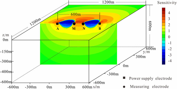
Figure 5. The distribution of three-dimensional influence coefficients of apparent resistivity observation area The influence coefficients are non-continuously distributed, with two approximately elliptical areas of negative influence coefficients between the measuring and power supply electrodes in both horizontal and vertical directions, while the coefficients in the other areas are positive. The influence coefficients (in absolute value) are the greatest near the electrodes and decrease rapidly in the areas far from the measurement line. Additionally, the influence coefficients exhibit symmetry in the direction perpendicular to the measurement line.
The three-dimensional distribution of influence coefficients is directly influenced by the positioning of electrodes. Notably, a negative region exists between the power supply electrode and the measuring electrode, a characteristic determined by the device layout rather than guiding the arrangement of the observation system itself. However, understanding the distribution characteristics of these coefficients can aid in selecting measurement areas to avoid potential interference sources based on their locations.
Based on the theory of influence coefficients, the various parameters of the apparent resistivity observations at Hefei seismic station were substituted into Equations 5, 6 to obtain the one-dimensional influence coefficient model for Hefei Station (Figure 6).
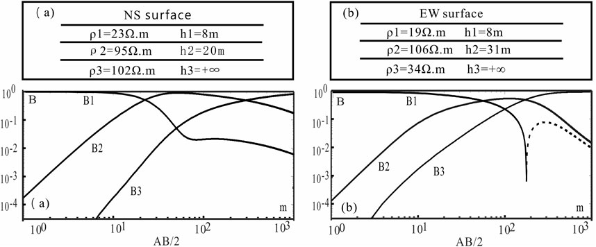
Figure 6. Horizontal layered model and its one-dimensional influence coefficient of Hefei station. The layered structure and one-dimensional influence Coefficient of the observation site are inversed according to the electric sounding curve, where (A) is in NS direction and (B) is in EW direction. B1 is the first coefficient, and so on.
Based on the calculation results from Figure 6, at the Hefei station, the apparent resistivity measurement distance between the electrodes A and B is 600 m, at this time:
In the NS direction it can be represented as Equation 13.
In the direction of EW it can be represented as Equation 14.
In the analysis of one-dimensional influence coefficients, the influence coefficient of the surface medium in the NS direction remains positive within the calculation range where the electrode distance AB/2 < 1,000 m. Conversely, in the EW direction, the influence coefficient of the surface medium is negative within the range where the electrode distance is between 190 m and 1,000 m. During the rainy season, the one-dimensional influence coefficient analysis indicates that apparent resistivity observation decreases in the NS direction, while it increases in the EW direction.
Based on the one-dimensional influence coefficients, the coefficients for the surface and sub-surface layers in the NS direction are positive. The pumping of water from the reservoir can be understood as a decrease in water level between the NS directions. The pumping operation is equivalent to the water in the reservoir area turning into air. At this time, the apparent resistivity of the reservoir should increase, but the apparent resistivity data decreases instead, causing a deviation between the theoretical and actual values. Therefore, in October 2018, when the reservoir between the power supply electrode B and the measuring electrode N was pumped, this resulted in a change in the local medium’s resistivity in the measurement area, which is not a change in the entire layer, and at this time, it no longer meets the analysis conditions of the one-dimensional influence coefficient.
Since the results obtained from the traditional one-dimensional influence coefficient analysis have deviated, according to the method described in Section 3.3, a finite element analysis method is applied to calculate the three-dimensional influence coefficients, thereby obtaining the distribution of the three-dimensional influence coefficients for the NS direction apparent resistivity site. Based on electrical sounding data, the finite element analysis method was employed to compute the three-dimensional influence coefficients, resulting in a distribution for the NS direction apparent resistivity site, as illustrated in Figure 5. The reservoir lies entirely within the negative influence coefficient region between the power supply electrode B and the measuring electrode N. This indicates that the increase in the reservoir’s resistivity leads to a decrease in observed values, aligning with actual observations. The size of the reservoir is approximately 30 m * 30 m * 25 m. Using the constructed three-dimensional finite element model, the impact of water pumping on the apparent resistivity values of the NS direction is quantitatively calculated (Table 2). Through the calculations in Table 2, the calculated values match the observed values and the magnitude of change, which indicates that the anomalous variation in the apparent resistivity observation at the Hefei station in 2018 was caused by water pumping, rather than anisotropic variation. Future efforts can utilize finite element quantitative calculations to refine estimates of impact magnitude more precisely.
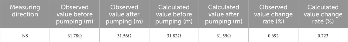
Table 2. Observed values and quantitative calculated values before and after water pumping in 2018.
Following the pumping of the reservoir, the water level gradually recovered through natural replenishment, including rainfall. As air within the reservoir was replaced by water, the resistivity of the reservoir decreased. Considering the negative characteristics of the three-dimensional influence coefficients, the observed apparent resistivity should have continued to increase, consistent with actual observations. Hence, the apparent resistivity anomalies observed at Hefei Station are attributed to environmental changes rather than anisotropy.
Since 1966, China has been using apparent resistivity observations to forecast strong aftershocks of the Xingtai earthquake. This was followed by the Ms7.8 Tangshan earthquake in 1976, the Ms7.2 Songpan-Pingwu earthquake in 1976, and the Ms7.6 Lancang-Gengma earthquake in 1988. Before these earthquakes, significant anomalies in apparent resistivity were recorded, and retrospective studies have shown that these anomalies typically exhibit anisotropic characteristics before earthquakes. Before the occurrence of major earthquakes, anisotropic changes in apparent resistivity are observed at stations near the epicenter, which is consistent with experimental results (Zhao et al., 1995; Qian et al., 1996; Du et al., 2007) and has been confirmed by many earthquake cases. For example, before the Ms8.0 Wenchuan earthquake in 2008, it was known that the Chengdu and Jiangyou stations were about 35 Km and 30 Km away from the main rupture zone, respectively. According to the existing segmentation source mechanism solution of the main shock, the main compressive stress direction near the Chengdu station is N51°W, and near the Jiangyou station is N5°W (Zhang et al., 2009). The observation direction of the Chengdu station at N58°E forms an angle of 71° with the main compressive stress axis, with the maximum decrease before the earthquake being about 7%; the observation direction at N49°W is nearly parallel to the main compressive stress axis, and no decrease was observed before the earthquake. The observation direction of the Jiangyou station at N70°W forms an angle of 65° with the main compressive stress axis, with a decrease of about 1.5% before the earthquake, while the observation direction at N10°E is roughly parallel to the main compressive stress axis, showing no significant anomalous decrease before the earthquake (Lu et al., 2016; Xie et al., 2018).
At the same time, interferences encountered in apparent resistivity observations may also exhibit anisotropic changes. Since both interferences and pre-seismic stress changes can cause anomalous data changes, it is essential to first exclude interferences when data anomalies occur. Common interferences include metal pipelines within the measurement area, subway operation interference, and rainfall interference, among which rainfall interference affects the entire observation area and usually does not produce anisotropic changes. However, subway operation interference and metal pipeline interference within the measurement area can usually cause anisotropic changes in apparent resistivity observations.
This article analyzes the anisotropic anomalies in the apparent resistivity observations at the Hefei seismic station from October to December 2018 and establishes steps for analyzing anisotropic anomalies before earthquakes. First, determine the type and magnitude of the anomaly, then investigate existing sources of interference, and finally, conduct qualitative analysis and quantitative calculation. Through the above steps of model construction, interference can be excluded, thereby establishing a method for analyzing anisotropy in apparent resistivity before earthquakes. If the values are still anomalous after quantitative calculation to remove the effects of interference, it can be determined as anisotropic changes before the earthquake. The above analysis method still has guiding significance for anisotropic analysis of apparent resistivity at other stations.
For example, the Xingji seismic station in Hebei Province is located in the central-eastern part of Hebei Province, with two ground apparent resistivity measurement items of N30°E and N60°W, with a power supply electrode distance of 2 km and a measuring electrode distance of 0.5 km. There is a reservoir between the B electrode and the N electrode of the N60°W direction, which rises with the increase of rainfall in summer and falls in winter (Figure 7A). The precipitation in the area where the station is located is consistent over the years, and the seasonal change of the water level of the reservoir is also consistent. According to the influence coefficient analysis, the rise of the water level of the reservoir will cause an increase in the N60°W observation, so the seasonal change of the water level of the reservoir is an important influencing factor for the “high in summer and low in winter” trend of the N60°W observation (Figure 7C).
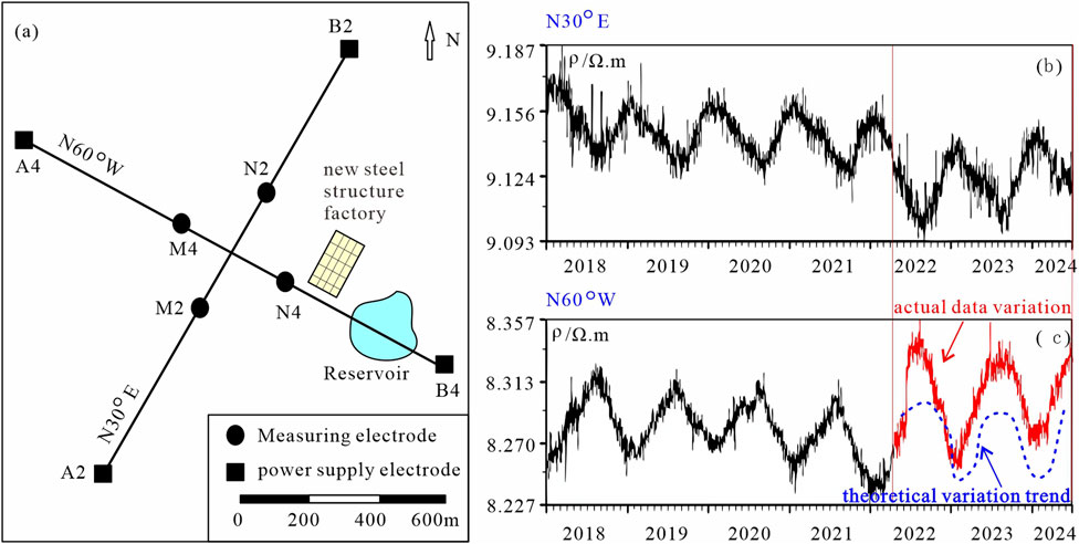
Figure 7. Apparent resistivity site conditions and historical data curves of Xingji seismic station from January 2018 to April 2024. (A) The layout of the external circuit site, the location of the reservoir, and the factory building. (B,C) illustrate the data variation trends for the N30°E and N60°W directions, respectively. The red curves represent the actual data variation, while the blue curves represent the theoretical variation trend.
In March 2022, the apparent resistivity observation of the N60°W direction at the Xingji seismic station showed a high-value change, breaking through the theoretical trend, while the observation of the N30°E direction was not significantly changed, forming anisotropic changes in the two directions (Figures 7B, C). After the data change, the observation system was checked for no faults. During the patrol of the observation environment, it was found that a steel structure factory building was newly built between the B electrode and the N electrode of the N60°W direction during this period. According to the models and methods in the text, the factory building is located in the area where the influence coefficient of the N60°W direction is negative and the influence coefficient of the N30°E direction is positive. Since the newly built factory building is closer to the N60°W direction, it has a greater impact on this direction, showing a significant increase in the N60°W observation while the N30°E observation remains basically unchanged. By calculating with the finite element method, the newly built steel structure factory building can cause the N60°W observation to rise by 0.07 Ω.m, so this anomaly is caused by the newly built factory building, not a pre-seismic anomaly. After the completion of the steel structure factory building, it has always existed, so the overall data of the N60°W direction is 0.07 Ω.m higher than before the construction of the factory building, and it will not return to the level before the construction of the factory building.
Currently, in addition to China conducting large-scale apparent resistivity observations, other countries that use apparent resistivity observations for earthquake prediction include the United States, Japan, Greece, and so on. However, international research on apparent resistivity anisotropy mostly focuses on the mechanisms by which anisotropy is generated (Sævik et al., 2014; Thongyoy et al., 2023). China has rich experience and successful cases in using apparent resistivity anisotropy for earthquake prediction (Du, 2010; Xu et al., 2014). At the same time, environmental interference such as subway operations near the observation area, metal pipeline networks, and water level changes are universally present in practice, and traditional one-dimensional influence coefficient analysis can no longer meet the needs. Thus, this study provides a reference for professionals in other regions internationally to use changes in apparent resistivity anisotropy for earthquake prediction. When using anisotropic apparent resistivity observation for forecasting work, it is important to identify the types of interference mentioned in the text and quantitatively remove interference factors. Additionally, it is recommended that when building apparent resistivity stations in seismic areas for earthquake prediction, efforts should be made to avoid areas with large local influence coefficients to ensure that pre-seismic anomaly data is truly reliable.
Based on the review of the theoretical development and application of apparent resistivity anisotropy, taking the observation of the Hefei seismic station in Anhui Province as an example, a model is constructed using the finite element method to establish a method for determining the pre-seismic apparent resistivity anisotropy. The observation from the Xingji Seismic Station in Hebei Province is used for verification, and the study concludes the following:
(1) Anomalous changes in anisotropic apparent resistivity observations do not necessarily indicate the occurrence of an earthquake; they could also be caused by interference within the observation site, including subway operations, reservoirs, metal pipelines, etc. Therefore, after an anomaly occurs, it is necessary to first investigate these sources of interference.
(2) Through calculation and analysis using the finite element method, on the two-dimensional surface plane of the apparent resistivity observation site, most areas have a positive influence coefficient. However, there are two roughly elliptical areas with a negative influence coefficient between the measuring and power supply electrodes. In three-dimensional space, there is a continuous area between the power supply and measuring electrodes that corresponds to the negative influence coefficient area on the surface. The distribution of the influence coefficient shows obvious symmetry, with the axis of symmetry being the midline of the electrode connection line, and the influence coefficient (in absolute value) is inversely proportional to the distance from the electrodes.
(3) Using the method in this paper, the water level changes in the reservoir within the observation area of the Hefei seismic station in Anhui Province can cause about 0.7% change in the NS direction observation, and the construction of the steel structure factory building in the direction of N60°W at the Xingji seismic station can cause a change of 0.07 Ω.m in the apparent resistivity observation. If the anomaly exceeds this amplitude, it should be considered as a pre-seismic anisotropic anomaly for earthquake prediction.
(4) This study can provide a reference for forecasters in other seismically active regions to quantitatively remove environmental interference factors in anisotropic anomalies. After an anomaly occurs, first investigate instrument faults, external line faults, environmental interference, and other aspects to identify the source of interference, and then quantitatively calculate the data change caused by the interference source to determine whether the data anomaly is entirely caused by interference. It is also recommended that when building apparent resistivity stations in seismic areas for earthquake prediction, efforts should be made to avoid areas with large local influence coefficients to ensure that pre-seismic anomaly data is truly reliable.
The original contributions presented in the study are included in the article/supplementary material, further inquiries can be directed to the corresponding author.
YL: Writing–original draft, Writing–review and editing. LJ: Writing–review and editing. CJ: Conceptualization, Writing–original draft. HD: Conceptualization, Writing–review and editing. CM: Data curation, Writing–original draft. JW: Data curation, Writing–original draft. MW: Conceptualization, Writing–review and editing.
The author(s) declare that financial support was received for the research, authorship, and/or publication of this article. China-Asean Earthquake Disaster Monitoring and Defense Capability Improvement Project (No. 123999101), third batch of Fengyun-3 meteorological satellite projects (No. FY-3(03)-AS-11.10-ZT) Anhui Provincial Key Research and Development Project (2022m07020002, 2022m07020005), Spark Program of Earthquake Sciences (XH23021YB), Three combined Project (3JH-202402004), The Seismic Pattern and Impact of the Tan-Lu Fault Zone in the Feidong-Lujiang section research project.
Author JW was employed by Geovis Environment Technology Co., Ltd.
The remaining authors declare that the research was conducted in the absence of any commercial or financial relationships that could be construed as a potential conflict of interest.
All claims expressed in this article are solely those of the authors and do not necessarily represent those of their affiliated organizations, or those of the publisher, the editors and the reviewers. Any product that may be evaluated in this article, or claim that may be made by its manufacturer, is not guaranteed or endorsed by the publisher.
Bachrach, R. (2011). Elastic and resistivity anisotropy of shale during compaction and diagenesis: joint effective medium modeling and field observations. Geophysics 76 (6), E175–E186. doi:10.1190/geo2010-0381.1
Coggon, J. H. (1971). Electromagnetic and electrical modeling by the finite element method. Geophysics 36, 132–155. doi:10.1190/1.1440151
Crampin, S., Evan, R., and Atkins, B. K. (1984). Earthquake prediction: a new physical basis. Geophys. J. R. Astronomical Soc. 76, 147–156. doi:10.1111/j.1365-246x.1984.tb05016.x
Dey, A., and Morrison, H. F. (1979). Resistivity modeling for arbitrarily shaped three-dimensional structures. Geophysics 44 (4), 753–780. doi:10.1190/1.1440975
Du, X.-b. (2010). Two types of changes in apparent resistivity in earthquake prediction. Sci. China 40 (10), 1321–1330.
Du, X.-b., Li, N., Ye, Q., Ma, Z.-h., and Yan, R. (2007). A possible reason for the anisotropic changes in apparent resistivity near the focal region of strong earthquake. Chin. J. Geophys. 50 (6), 1802–1810. doi:10.3321/j.issn:0001-5733.2007.06.021
Du, X.-b., Sun, J.-s., and Chen, J.-y. (2017). Data processing method of Earth resistivity in earthquake prediction. Acta Seismo Sin. 39 (4), 531–548. doi:10.11939/jass.2017.04.008
Ellis, M. H., Sinha, M. C., Minshull, T. A., Sothcott, J., and Best, A. I. (2010). An anisotropic model for the electrical resistivity of two-phase geologic materials. Geophysics 75 (6), E161–E170. doi:10.1190/1.3483875
Kemeny, J. M. (1991). A model for non-linear rock deformation under compression due to sub-critical crack growth. Int. J. Rock Mech. Min. Sci. Geomech. Abstr. 28 (6), 459–467. doi:10.1016/0148-9062(91)91121-7
Kenneth, L. C., and Russell, L. G. (1961). Theoretical horizontal resistivity profiles over hemispherical sinks. Geophysics 9 (3), 342–354. doi:10.1190/1.1438877
Kraev, A. (1954). in Geoelectrical principles, Z. Ke-qian, C. Pei-guang, and Z. Zhi-cheng (Beijing: Geological Publishing House).
Li, Y. G., and Spitzer, K. (2005). Finite element resistivity modelling for three-dimensional structures with arbitrary anisotropy. Phys. Earth Planet. Interiors 150, 15–27. doi:10.1016/j.pepi.2004.08.014
Lu, J., Qian, F.-y., and Zhao, Y.-l. (1999). Sensitivity analysis of the Schlumberger monitoring array: application to changes of resistivity prior to the 1976 earthquake in Tangshan, China. Tectonophysics 307 (3-4), 397–405. doi:10.1016/s0040-1951(99)00101-8
Lu, J., Xie, T., Li, M., Wang, Y., Ren, Y., Gao, S., et al. (2016). Monitoring shallow resistivity changes prior to the 12 May 2008 M8.0 Wenchuan earthquake on the Longmen Shan tectonic zone, China. Tectonophysics 675, 244–257. doi:10.1016/j.tecto.2016.03.006
Lu, J., Xue, S.-z., Qian, F.-y., Zhao, Y., Guan, H., Mao, X., et al. (2004). Unexpected changes in resistivity monitoring for earthquakes of the Longmen Shan in Sichuan, China, with a fixed Schlumberger sounding array. Phys. Earth Planet. Interiors 145 (1-4), 87–97. doi:10.1016/j.pepi.2004.02.009
Ni, H.-y., Zheng, H.-g., Zhao, N., Deng, B., Miao, P., Huang, X.-l., et al. (2022). Application of ambient noise tomography with a dense linear array in prospecting active faults in the Mingguang city. Chin. J. Geophys. 65 (7), 2518–2531. doi:10.6038/cjg2022P0947
North, L. J., and Best, A. I. (2014). Anomalous electrical resistivity anisotropy in clean reservoir sandstones. Geophys. Prospect. 62 (6), 1315–1326. doi:10.1111/1365-2478.12183
O’Neill, D. J., and Merrick, N. P. (1984). A digital linear filter for resistivity sounding with a generalized electrode array. Geophys Prospect 32 (1), 105–123. doi:10.1111/j.1365-2478.1984.tb00720.x
Park, S. K., and Van, G. P. (1991). Inversion of pole-pole data for 3-D resistivity structure beneath arrays of electrodes. Geophysics 56 (7), 951–960. doi:10.1190/1.1443128
Qian, F.-y., Zhao, Y.-l., and Huang, Y.-n. (1996). Georesistivity anisotropy parameters calculation method and earthquake precursor example. Acta Seismol. Sin. 18 (4), 480–488.
Qian, J.-d., Chen, Y.-f., and Jin, A.-z. (1985). Application of Earth resistivity method in earthquake prediction. Beijing: Seismological Press.
Qian, J.-d., Ma, Q.-z., and Li, S. (2013). Further study on the anomalies in apparent resistivity in the NE configuration at Chengdu station associated with Wenchuan MS8.0 earthquake. Acta Seismol. Sin. 35 (1), 4–17. doi:10.3969/j.issn.0253-3782.2013.01.002
Sævik, P. N., Jakobsen, M., Lien, M., and Berre, I. (2014). Anisotropic effective conductivity in fractured rocks by explicit effective medium methods. Geophys. Prospect. 62 (6), 1297–1314. doi:10.1111/1365-2478.12173
Thongyoy, W., Siripunvaraporn, W., Rung-Arunwan, T., and Amatyakul, P. (2023). The influence of anisotropic electrical resistivity on surface magnetotelluric responses and the design of two new anisotropic inversions. Earth, Planets Space 75 (1), 12. doi:10.1186/s40623-023-01763-1
Xie, T., Liu, J., Lu, J., Li, M., Yao, L., Wang, Y.-l., et al. (2018). Retrospective analysis on electromagnetic anomalies observed by ground fixed station before the 2008 Wenchuan Ms8.0 earthquake. Chin. J. Geophys. 61 (5), 1922–1937. doi:10.6038/cjg2018M0147
Xie, T., and Lu, J. (2015). Three-dimensional influence coefficient of Earth resistivity and its application. Seismol. Geol. 37 (4), 1125–1135. doi:10.3969/j.issn.0253-4967.2015.04.015
Xie, T., and Lu, J. (2020a). Apparent resistivity anisotropic variations in cracked medium. Chin. J. Geophys 63 (4), 1675–1694.
Xie, T., Wang, H.-q., Liu, L.-b., and Lu, J. (2014). Inverse annual variations of apparent resistivity at Siping earthquake station by using finite method. Prog. Geophys. 29 (2), 588–594. doi:10.6038/pg20140215
Xie, T., Ye, Q., and Lu, J. (2020b). Electrical resistivity of three-phase cracked rock soil medium and its anisotropic changes caused by crack changes. Geomat. Nat. Haz. Risk 11 (1), 1599–1618. doi:10.1080/19475705.2020.1801527
Xu, X.-q., Gao, C.-z., and Wang, L. (2014). Study on long-term observation data of Earth resistivity at baochang station, inner Mongolia. J. Earthq. Eng. 36 (2), 405–412. doi:10.3969/j.issn.1000-0844.2014.02.0405
Yao, W.-b. (1989). Introduction to numerical computation and interpretation of electrical sounding. Beijing: Seismological Press, 85–94.
Zhang, X.-m., Li, M., and Guan, H.-p. (2009). Analysis of Earth resistivity anomalies before the wenchuan county M8.0 earthquake. Earthquake 29 (1), 108–115. doi:10.3969/j.issn.1000-3274.2009.01.014
Zhang, Y., Xu, L.-s., and Chen, Y.-t. (2009). Spatio-temporal variation of the source mechanism of the 2008 great Wenchuan earthquake. Chin. J. Geophys. 52 (2), 379–389.
Zhao, Y.-l., Li, Z.-n., and Qian, F.-y. (1995). Comprehensive criteria for the transition from the middle-term to the short-term and impending anomalies of geoelectric precursors. Earthquake 4, 308–314.
Keywords: finite element, apparent resistivity, influence coefficient, layered medium, anisotropy
Citation: Lei Y, Jianyong L, Junfeng C, Dequan H, Manfeng C, Wei J and Weiyu M (2024) Analysis of anisotropy anomalies identification in apparent resistivity observation. Front. Earth Sci. 12:1423823. doi: 10.3389/feart.2024.1423823
Received: 26 April 2024; Accepted: 29 August 2024;
Published: 13 September 2024.
Edited by:
Giovanni Martinelli, Section of Palermo, ItalyReviewed by:
Vincenzo Lapenna, National Research Council (CNR), ItalyCopyright © 2024 Lei, Jianyong, Junfeng, Dequan, Manfeng, Wei and Weiyu. This is an open-access article distributed under the terms of the Creative Commons Attribution License (CC BY). The use, distribution or reproduction in other forums is permitted, provided the original author(s) and the copyright owner(s) are credited and that the original publication in this journal is cited, in accordance with accepted academic practice. No use, distribution or reproduction is permitted which does not comply with these terms.
*Correspondence: Li Jianyong, anlsaUBzZWlzLmFjLmNu
Disclaimer: All claims expressed in this article are solely those of the authors and do not necessarily represent those of their affiliated organizations, or those of the publisher, the editors and the reviewers. Any product that may be evaluated in this article or claim that may be made by its manufacturer is not guaranteed or endorsed by the publisher.
Research integrity at Frontiers
Learn more about the work of our research integrity team to safeguard the quality of each article we publish.