A comparative study of regional rainfall-induced landslide early warning models based on RF、CNN and MLP algorithms

Landslide disasters, due to their widespread distribution and clustered occurrences, pose a significant threat to human society. Rainfall is considered a primary triggering factor, and the frequent clustering of landslides underscores the importance of early warning systems for regional landslide disasters in preventing and mitigating rainfall-induced landslides. Research on early warning models is crucial for accurately predicting rainfall-induced landslides. However, traditional models face challenges such as the complexity of landslide causes, insufficient data, and limited analysis methods, resulting in low accuracy and inadequate precision. This study focuses on Fujian Province, China, proposing a four-step process for building a regional landslide early warning model based on machine learning. The process includes data integration and cleaning, sample set construction, model training and validation, and practical application. By integrating and cleaning the latest and most detailed data, a training sample set (15,589 samples) for the regional landslide disaster early warning model is established. Three machine learning algorithms—Random Forest, Multilayer Perceptron, and Convolutional Neural Network—are employed and compared, the evaluation results indicated that the RF-based warning model achieved an accuracy of 0.930–0.957 and an AUC value of 0.955. The CNN-based warning model demonstrated an accuracy of 0.945–0.948 with an AUC value of 0.940. The MLP-based warning model achieved an accuracy of 0.930–0.953 and an AUC value of 0.930. The results showed comparable accuracy metrics among the three models, with RF exhibiting a significant advantage in AUC values. Finally, the models are applied to the regional landslide disasters induced by heavy rainfall in Fujian Province on 5 August 2021. The results showed that in the binary classification warning strategy, the accuracy of the Random Forest and Convolutional Neural Network was 92.9%, while that of the Multilayer Perceptron was 85.8%, all performing well. In the multi-classification hierarchical warning strategy, the Random Forest excelled, while the performance of the Convolutional Neural Network and Multilayer Perceptron was relatively limited. The findings of this study contribute to valuable attempts in landslide disaster warning model research, with anticipated further improvements through the gradual accumulation of samples and practical application verification.

1 Introduction

Landslide disasters often result in the destruction of houses, disruption of transportation routes, and pose a serious threat to the safety of people’s lives and property (Froude and Petly, 2018; Gatto et al., 2023). Given the predominant triggering effect of rainfall and the frequent clustering of landslides in specific regions, early warning systems for regional rainfall-induced landslide disasters have become a critical tool in landslide disaster prevention, often referred to as the primary defense against such disasters. Research on landslide disaster early warning models is essential for accurate predictions. Based on this, numerous scholars both domestically and internationally have conducted extensive research on this matter. For example, Caine studied the rainfall intensity-duration control of shallow landslides and debris flows (Caine, 1980).

The earliest applied model is the statistical critical rainfall threshold model (Cannon, 1985; Au, 1998; Aleotti, 2004; Krøgli et al., 2018; Baum and Godt, 2010; Abraham et al., 2020). Due to its simplicity, this model has been widely referenced and applied in various regions (Liu et al., 2015; Hong et al., 2016a; Ding et al., 2017; Peruccacci et al., 2017; Wei et al., 2018). Other models, such as dynamic warning models, analyze the mechanism of rainfall-infiltration-disaster occurrence, primarily based on the mechanics of infinite slope stability analysis. These models couple rainfall-infiltration hydrogeological models with infinite slope stability mechanics to assess landslide stability (Ponziani et al., 2013; Pennington et al., 2015; Mulyana et al., 2019). Despite their clear physical significance, their complex parameter inputs and uncertainties limit their use to small-scale studies.

In recent years, the vigorous development of artificial intelligence technology has led to the maturation and widespread application of machine learning algorithms across various industries, including geological disaster prevention and control. Machine learning algorithms such as artificial neural networks, decision trees, support vector machines, and Random Forests have been extensively used for landslide spatial evaluation and prediction (Chen et al., 2017; Tien Bui et al., 2016, 2017; Liu et al., 2010; Hong et al., 2016a; Trigila et al., 2015; Dong et al., 2024; Zeng et al., 2024; Luti et al., 2020). For instance, Reichenbach et al. (2018) provided a comprehensive review of statistically-based landslide susceptibility models, while Ado et al. (2022) and Lima et al. (2022) offered extensive literature surveys and bibliometric analyses on machine learning applications in landslide susceptibility mapping. Yilmaz (2009) used frequency ratio, logistic regression, and artificial neural networks to generate landslide susceptibility maps in Tokat County, Turkey, with the artificial neural network model demonstrating superior performance. Micheletti et al. (2014) applied adaptive support vector machines, Random Forests, and AdaBoost for landslide susceptibility mapping in the Canton of Vaud, Switzerland. Thai Pham et al. (2019) used ensemble learning algorithms to assess susceptibility in Pithoragarh, India.

Furthermore, studies have integrated various machine learning techniques with physical models for enhanced accuracy. For instance, Jie Dou et al. (2015) combined the Certainty Factor method with ANN technology for Sado Island, Japan. In Austria, J.N. Goetz et al. (2015) found that Random Forest algorithms yielded the highest accuracy for landslide susceptibility mapping. Miloš Marjanović et al. (2009) and Sameen et al. (2020) used support vector machines, k-nearest neighbors, and Convolutional Neural Networks for regional assessments. Wei et al. (2021) developed a hybrid framework for regional landslide susceptibility mapping that combines physical models with Convolutional Neural Network.

Recent advancements have also focused on hybrid models that integrate machine learning with dynamic rainfall indices for improved early warning systems. Sun et al. (2022) proposed a coupled model using Random Forest susceptibility and precipitation factors, while Zhou et al. (2022) introduced an interpretable model combining SHAP and XGBoost for global and local susceptibility assessment. Yang et al. (2024) explored the CGBOOST deep-learning algorithm, and Liu et al. (2022) validated the feasibility of various machine learning algorithms for regional early warning models. Yuan and Chen (2023) proposed a national-level early warning method using hybrid neural networks and a spatiotemporal transformer.

Additionally, Khan et al. (2022) developed a global landslide forecasting system for hazard assessment and situational awareness. Nocentini et al. (2023) explored the influence of rainfall parameters and model settings on landslide space-time forecasting through machine learning. Ren et al. (2024) combined dynamic rainfall indices with machine learning methods for spatiotemporal landslide susceptibility modeling. Lee et al. (2022) integrated rainfall period, accumulated rainfall, and geospatial information for dynamic landslide susceptibility analysis.

In summary, early warning systems for rainfall-induced landslides are vital for disaster prevention. While traditional models have laid the groundwork, the integration of machine learning algorithms and hybrid models has significantly advanced the field, offering more accurate and scalable solutions for landslide prediction and risk assessment.

However, the aforementioned warning models face challenges such as the complexity of geological disaster causes, insufficient sample data, and limited analysis methods, resulting in low warning accuracy and inadequate precision. To address these issues, this paper introduces a four-step process for constructing a regional landslide early warning model based on machine learning. The steps include data integration and cleaning, construction of training sample sets, model training and validation, and practical application of the model. The study focuses on Fujian Province, one of the provinces in the southeast of China with a high frequency of landslide disasters, providing a comprehensive demonstration of the four-step process for building landslide warning models using three algorithms: Random Forest (RF), Convolutional Neural Network (CNN), and Multilayer Perceptron (MLP). By applying these algorithms, the paper conducts a comparative study using real-world examples, highlighting the advantages and disadvantages of each model in the context of binary and multiclass landslide disaster early warning strategies. This research represents a valuable attempt to integrate AI technology and machine learning algorithms into the field of landslide disaster early warning.

2 Geological background of the study area

China is one of the countries globally with the most extensive distribution and severe consequences of geological disasters (Liu et al., 2022). Landslide geological disasters are widespread in the mountainous and hilly areas across the country, with nearly a million known occurrences. On average, these landslides cause hundreds of deaths and result in direct economic losses amounting to tens of billions of yuan each year (Geological Hazard Technical Guidance Center, Ministry of Natural Resources, 2019). Fujian Province is one of the provinces in China where landslides occur frequently.

The geographical location of Fujian Province lies mainly in the hilly mountainous area along the southeast coast of China (as shown in Figure 1). Mountainous areas in Fujian Province account for 80.06% of the total land area, plains cover 8.03%, plateaus occupy 1.99%, and hills make up 9.92%. The distribution of terrain in the study area is uneven, with hills and mountains mainly concentrated in the central and western regions of Fujian Province, totaling approximately 106,244 square meters in area. The elevation generally ranges from 5 to 2,180 m. In the western part, the prominent feature is the Wuyi Mountains, which run horizontally and are located near the border between Jiangxi Province and Fujian Province. The Huanggang Mountain, with an altitude of approximately 2,158 m, is one of the main peaks. In the central part, there are mountain ranges such as the Shengfeng Mountain-Daiyun Mountain-Boping Ridge, which run in a north-northeast direction, consistent with the direction of the coastline. In comparison to the central and western regions of Fujian Province, the southeastern coastal area has relatively lower elevations, characterized mainly by terrain features such as hills, plateaus, and plains. The stratigraphy and lithology of Fujian Province are highly developed, with predominant rock types including granite, shale, sedimentary rock, metamorphic rock, sandstone, tuff, and ignimbrite. In the southwestern part of Fujian Province, there are thin layers of relatively soft mudstone and shale, while the central and southern regions are primarily composed of granite. Sedimentary and metamorphic rocks dominate in the western parts, and tuff and ignimbrite are predominant in the eastern parts. Fujian Province experiences a subtropical monsoon climate characterized by warm and humid conditions with abundant rainfall. Summers are hot and humid, autumns are rainy, and winters are relatively dry. The province receives ample precipitation, with an annual average ranging from 1,000 to 2,500 mm, with higher rainfall in summer and autumn and lower in spring and winter. The geological environmental factor map is shown in Figure 2 (modified by Liu et al., 2022).

Figure 1

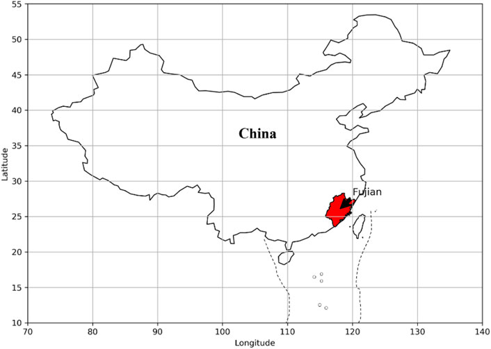
Figure 1. The geographical location of Fujian Province.

Figure 2

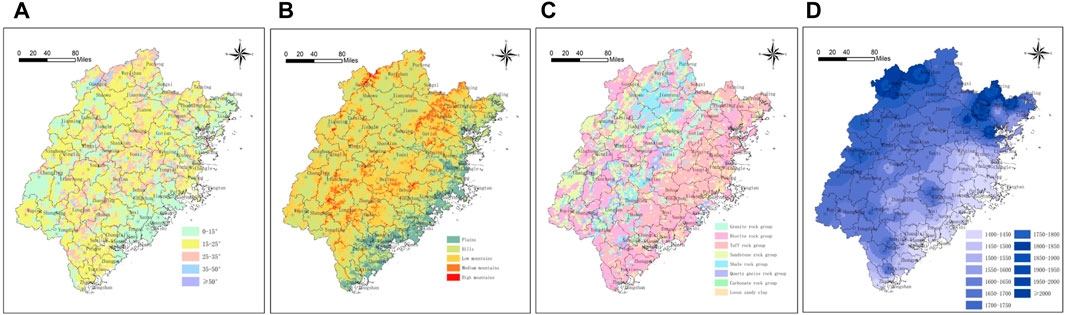
Figure 2. Geological environmental factor map (A): grade; (B) geomorphic type; (C) formation lithology; (D): annual rainfall.

In recent years, geological disasters have occurred frequently in Fujian Province, with collapses, landslides, debris flows, and ground collapses being the most common types, and the majority of them are of medium and small scale. Among them, landslides are the most significant type of natural disaster. By the end of 2019, a total of 21,176 geological disasters including collapses, landslides, debris flows, and ground collapses had occurred in the province.

3 Research methods and processes

The process of constructing the regional landslide warning model based on machine learning involves four main steps: data integration and cleaning, creation of a training sample set, development and validation of machine learning models, and practical application of the model. The specific structure and workflow are depicted in Figure 3.

Figure 3

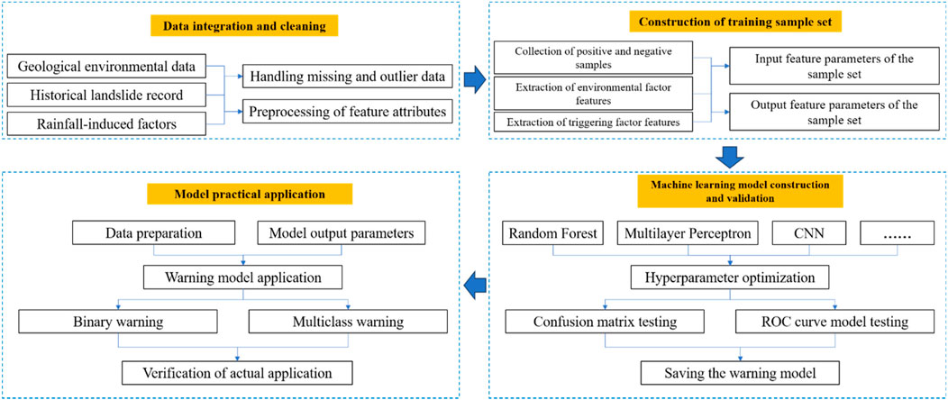
Figure 3. Schematic overview of the overall framework.

3.1 Data integration and cleaning

Building the training sample set for regional landslide warning mainly involves three types of datasets: geological environmental data, historical landslide records, and rainfall-triggering factors. Before constructing the sample set, it is necessary to collect, organize, and clean these three types of data. Data cleaning typically encompasses two categories:

(1) Data Missing and Anomaly Handling: Problems such as human errors, data transmission errors, equipment failures, and ambiguous geological information can impact the integrity of the original dataset. These issues need to be addressed through data preprocessing and cleaning. Typically, this involves dealing with missing values through interpolation or deletion, as well as identifying and correcting outliers.

(2) Feature Attribute Preprocessing: Given the varying scales of input features in the training samples, it is essential to standardize or scale these features uniformly. Different machine learning algorithms react differently to variations in input feature scales, necessitating distinct preprocessing methods for input feature attributes. It is significant to uniformly normalize or scale the input features of training samples before model training to minimize differences in feature ranges. Otherwise, this could directly impact the model’s accuracy.

The study focused on Fujian Province, China, and collected and organized historical landslide records, geological environmental data, and rainfall data. The landslide disaster data were sourced from the Fujian Province Landslide Disaster Sample Database spanning from 2010 to 2018. Landslides are distributed across all counties and districts in Fujian, but their frequency varies significantly. In the western, northern, and central regions of Fujian, the number of landslides is higher, mainly due to the rugged terrain and complex geological conditions in these areas, leading to more developed landslides. Specifically, in Youxi County, Datian County, and Dehua County in the central region, landslide occurrences exceed 300 times. In most other areas, the occurrences are below 150 times. However, in the southeastern coastal areas of Fujian, where the terrain is flat with predominantly plains and plateaus, landslide disasters are less likely to occur due to the flat terrain. The highest number of landslides in Fujian Province occurred in 2011, with 2,456 incidents, while the lowest number was in 2018, with only 39 incidents. The number of landslides in 2011 was 63 times that of 2018. Landslides in Fujian are mostly concentrated between May and August, accounting for 76% of the annual total. This is mainly due to Fujian’s subtropical monsoon climate, where the rainy season occurs from May to August. Rainfall is a significant factor in landslide disasters as it infiltrates the soil, reducing its strength and making it prone to permeation deformation, leading to soil failure and resulting in landslides. It has been observed that landslide occurrences are primarily influenced by heavy rainfall.

Data cleaning involved standardizing temporal and spatial coordinates, handling erroneous attribute values, and addressing missing fields in the historical landslide data. Geological environmental data were obtained from the 1:20,000 and 1:50,000 geological environment and geological disaster investigation databases of Fujian Province. Besides routine error data cleaning, preprocessing steps such as projection standardization, feature scaling, and normalization were conducted. Rainfall data were sourced from hourly meteorological and hydraulic rainfall station data from 2010 to 2018. Data cleaning tasks primarily included site registration, interpolation of missing data, and elimination of erroneous data. As shown in Table 1.

Table 1

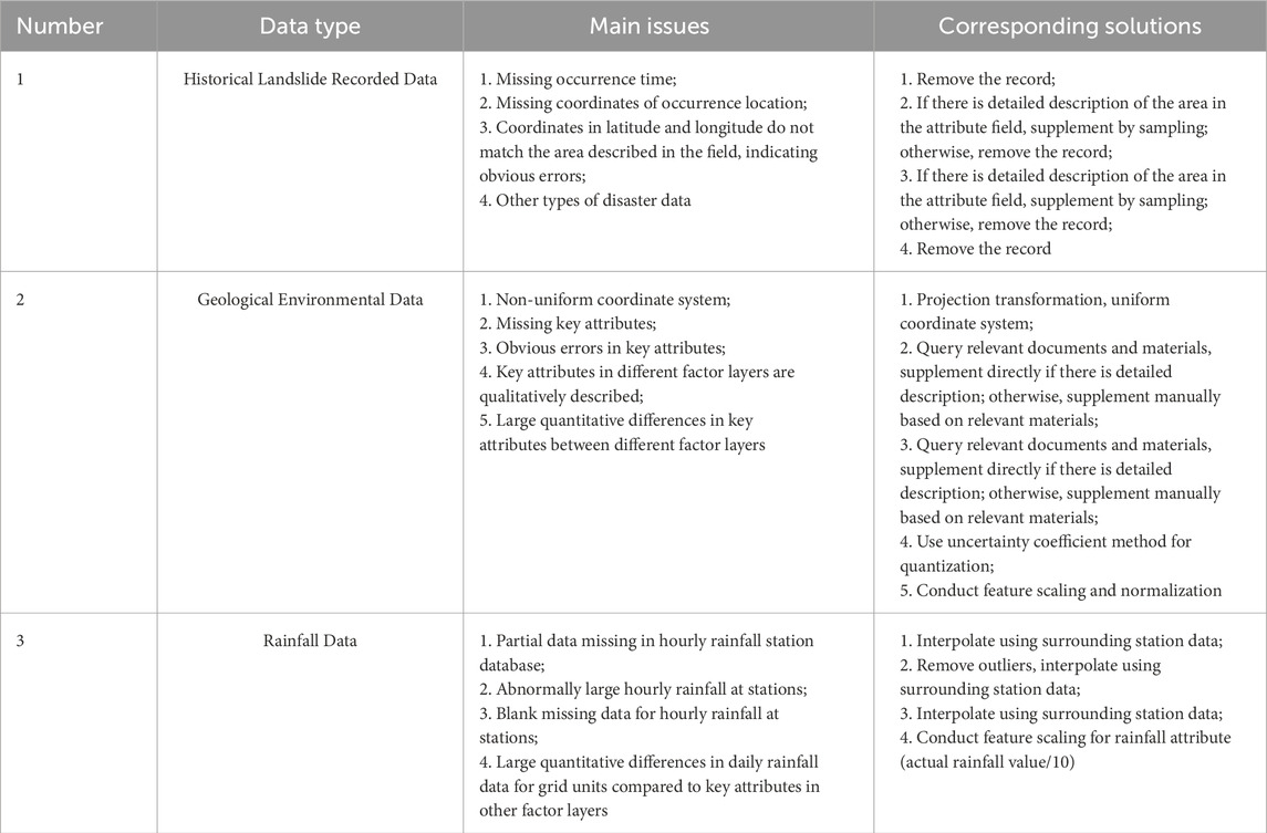
Table 1. Main issues and corresponding solutions for data Existence.

3.2 Construction of training sample set

The construction of the training sample set involves extracting environmental factor features and triggering factor features based on sampling of positive and negative samples, to obtain input and output feature parameters for the model. To construct the warning model, it is necessary to divide the sample data into training and testing sets. The optimized samples are randomly mixed and shuffled to ensure that the ratio of positive to negative samples in the training and testing sets is nearly consistent, preventing an imbalance in the number of positive and negative samples in either set. This study employs the model_selection module from sklearn using the Python language to divide all the landslide warning samples in the Fujian Province region into training and testing sets at a 4:1 ratio. To maintain consistency in the ratio of positive to negative samples within the training data, a specific percentage of each category’s samples is selected as training data. Since the model requires multiple training sessions, and to avoid changes in the training data due to random shuffling of the dataset each time, we use a fixed random_state. This ensures that the division of data remains the same for each training session.

3.2.1 Sampling of positive and negative samples

Positive sample sampling is based on historical landslide record data. According to the requirements of model construction, the selection criteria are as follows: the points must have definite spatial geographic coordinates and time coordinates (accurate to each day). Negative samples refer to points where landslides did not occur, which cannot be directly obtained. Negative sample sampling includes the following steps. See Figure 4 for a schematic diagram.

(1) Negative Sample Collection Outside the Buffer Zone of Positive Samples

Figure 4

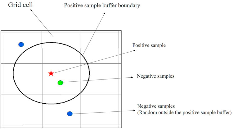
Figure 4. Schematic diagram of negative sample spatial sampling based on positive samples (modified by Liu et al., 2022)

Determination of Negative Sample Spatial Location: Negative samples are randomly sampled outside a certain buffer zone around positive samples. The determination of the buffer zone radius should consider both the minimum warning grid unit size in the study area and the distribution of historical landslide points.

Assignment of Time Attributes to Negative Samples: The time attributes of negative samples are typically constrained within the range of time distribution of positive samples. Sampling is conducted using a random function, with the general formula:

$\mathrm{T}=\text{RAND}\left({\mathrm{T}}_1,{\mathrm{T}}_2\right)$

T is the randomly obtained time; T1 is the lower limit of the period for randomly obtaining time; T2 is the upper limit of the period for randomly obtaining time.

(2) Negative Sample Collection Within the Grid of Positive Samples

Determination of Negative Sample Spatial Location: Negative samples are randomly sampled within the grid of positive samples, where the grid represents the warning grid units in the study area. The number of negative samples collected can be determined according to research requirements.

For the sampling of negative samples in this section, it is recommended to use the same number of negative samples as positive samples, meaning a 1:1 sampling ratio within grid units containing positive samples. However, this ratio should be specifically studied based on the particular research question, taking into account the varying number of samples in different study areas. Researchers are advised to collect and construct training sample sets based on different sampling ratios, and then select the optimal positive to negative sample ratio based on the model training results.

Assignment of Time Attributes to Negative Samples: For this portion, the time attributes of negative samples also use the random function shown in formula (1). However, in addition to the upper and lower limits of the period, an additional constraint is added: the time attribute of the sampled negative samples should be different from that of the positive samples.

In this study on early warning research in Fujian Province, the minimum warning grid unit is set to 2 km. In some regions, the density of historical landslide points is relatively high, so the buffer zone radius is set to the size of the warning grid unit, which is 2 km. To ensure the balance between positive and negative samples, the number of negative samples collected outside the buffer zone of positive samples is approximately twice the number of positive samples, while the number of negative samples collected within the grid of positive samples is equal to the number of positive samples. In summary, a total of 15,589 samples covering nearly 9 years (2010–2018) were obtained for Fujian Province. Among them, there are 3,562 positive samples and 12,027 negative samples, resulting in a positive-to-negative sample ratio of approximately 1:3.4. The spatial distribution of positive and negative samples is shown in Figure 5.

Figure 5

Figure 5. Location and training sample set of Fujian province.

3.2.2 Extraction of model input and output feature parameters

The model’s input feature parameters primarily encompass geological environmental factors, rainfall-triggering factors, and historical disaster information. The extraction of geological environmental features and rainfall factors is predicated on an analysis of the developmental distribution patterns and influencing factors of landslide disasters in the study area. Geological environmental factors influencing landslide disasters in the region typically comprise topography, lithology, and human activities. Rainfall-triggering factors influencing landslide disasters in the region generally encompass daily rainfall, antecedent rainfall, or antecedent effective rainfall.

Geological environmental factors and rainfall-triggering factors are overlaid and analyzed with the subdivision units of the warning grid (refer to Figure 6) to obtain the geological environmental features and rainfall factors of the warning grid units. The geological environmental feature database contains characteristic attributes of geological environmental factors for each warning grid unit, while the rainfall factor database includes daily rainfall feature attributes or effective rainfall feature attributes for each warning grid unit.

Figure 6

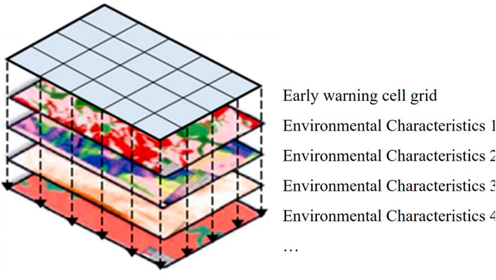
Figure 6. Schematic diagram of model input feature parameter extraction (modified by Liu et al., 2022)

The model’s output feature parameters are determined by the attributes of positive and negative samples. The output feature parameter for positive samples is set to 1, while the output feature parameter for negative samples is set to 0.

In the study area of Fujian Province, China, this paper extracted 10 feature factors including slope, landform type, lithology, annual rainfall, vegetation type, hydrological influence, roads, buildings, and actual occurrences of historical landslides (the actual number of historical disaster points in each grid unit) as input features representing geological environmental conditions. Additionally, 16 rainfall-triggering factors such as daily rainfall and rainfall over the previous 15 days were incorporated as input features for rainfall-triggering factors. This resulted in a total of 26 input feature attributes and one output feature attribute, comprising a training sample set of 15,589 records (see Figure 6; Table 2).

Table 2

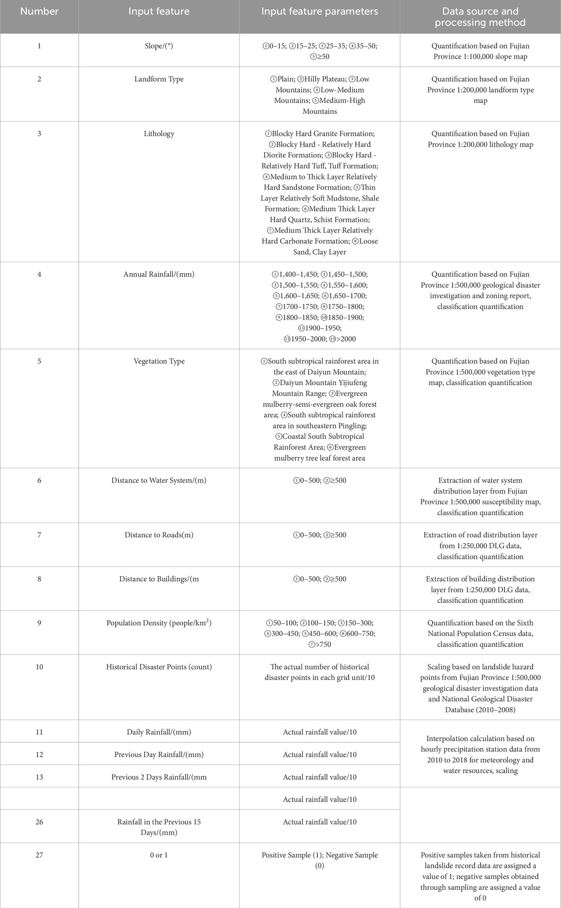
Table 2. Training sample input and output features and parameters (modified by Liu et al., 2022).

During the process of dividing the sample data into training and testing sets, the optimized samples were randomly mixed to ensure that the ratio of positive and negative samples in both the training and testing sets was consistent. This was done to prevent any imbalance in the number of positive and negative samples in either the training or testing set. The division of the Fujian Province landslide warning sample set into training and testing sets was accomplished using the model_selection module in sklearn, implemented in Python. The dataset was divided in a 4:1 ratio. To ensure a balanced ratio of positive and negative samples in the training data, a specific percentage was extracted from each class of samples as training data. To maintain consistency in data division across multiple training iterations and avoid variations caused by random shuffling of the dataset, a fixed random_state was employed to ensure consistent results in each training division.

The above content selected 26 indicators as input features, but different features have varying levels of importance and impact on the model. To investigate the influence of input features on the model and determine whether the selected input features are appropriate, a study on the importance of input features was conducted using the Random Forest algorithm model as an example.

The process for selecting input features is as follows:

First, calculate the importance of each input feature. The formula for calculating the importance index is as follows:

$P_k=\frac{{\sum }_{i=1}^n{\sum }_{j=1}^t{D}_{Gkij}}{{\sum }_{k=1}^m{\sum }_{i=1}^n{\sum }_{j=1}^t{D}_{Gkij}}\times 100\%$

Where P_k represents the importance of the k input feature; m is the number of input features; n is the number of decision trees; t is the number of nodes in each decision tree; D_Gkij is the decrease in Gini index for the k input feature at the j node of the i decision tree.

The importance of each input feature to the model output was calculated according to the Equation. The ranking of the importance of each input feature is shown in Figure 7.

Figure 7

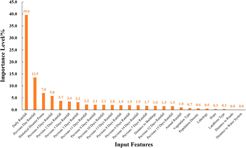
Figure 7. The importance of the input features.

The importance indices of the 26 input features in the study area can be ranked into six levels:

Level 1: Rainfall on the current day and the previous day, with importance indices of 39.6% and 13.5%, respectively.

Level 2: Distribution of historical disaster points, with an importance index of 7.0%.

Level 3: Rainfall from the second to the fifth day before, with importance indices ranging from 3.2% to 5.8%.

Level 4: Rainfall from the sixth to the 15th day before, distance to houses, and average annual rainfall, with importance indices ranging from 1.0% to 2.2%.

Level 5: Vegetation type, population density, strata lithology, slope, and geomorphological type, with importance indices ranging from 0.3% to 0.7%.

Level 6: Distance to roads and distance to water systems, with the lowest importance indices, both less than 0.1%.

The analysis of the importance ranking of each input feature is closely related to the study scale. At the provincial scale of this study in Fujian (with 2 km*2 km warning grid units), the input features in Level 5 are larger-scale geological environmental factors with relatively smaller impacts. Additionally, the landslide samples collected are mainly located near residential areas, while landslides along roads were not included, directly resulting in the importance indices of distance to roads and distance to water systems being close to 0. The high importance values of features such as rainfall on the current day, distribution of historical disaster points, rainfall from the first to the fifth day before, and distance to houses align with the recognized patterns of landslide disasters and triggering factors in Fujian Province. Using the recursive elimination method, the input feature with the smallest importance indicator was removed each time, and the optimized Random Forest algorithm was used to calculate the model accuracy. The results showed that the model accuracy remained largely unchanged after removing some features. Considering that the number of input features in this study is not large, all 26 input features were retained for the subsequent model.

3.3 Model construction and validation

This paper develops warning models using three machine learning algorithms: the Random Forest model, the Convolutional Neural Network (CNN) model, and the Multilayer Perceptron (MLP) model. The Random Forest model is an ensemble learning technique that combines weak learners (decision trees) by randomly sampling data and aggregating their outputs through voting to produce the final prediction. The Convolutional Neural Network (CNN) is a type of feedforward neural network commonly used in image recognition, speech recognition, and various other applications. It comprises layers such as convolutional layers, pooling layers, fully connected layers, as well as input and output layers. The Multilayer Perceptron (MLP) model consists of multiple layers of neurons, each resembling an artificial neural network layer. Neurons within each layer receive inputs from the preceding layer, apply nonlinear transformations via activation functions, and pass the results to the subsequent layer, enabling effective solutions to nonlinear problems.

3.3.1 Random Forest model

The Random Forest algorithm employs bootstrapping, where n samples are randomly selected with replacement to form k new sample training sets. This ensures that decision trees within the Random Forest can distinguish between each other, thus increasing the diversity of the decision trees and enhancing the reliability of the analysis results, thereby improving model performance. These k-decision trees are then combined into a Random Forest through ensemble algorithms. Subsequently, each of the sample mentioned above sets is used as a training set, and decision tree models are applied to train these samples. By evaluating the output probability values, the best decision tree nodes are selected for splitting. Finally, the results generated by all decision trees are combined using a simple majority voting mechanism to obtain the final result. As shown in Figure 8.

Figure 8

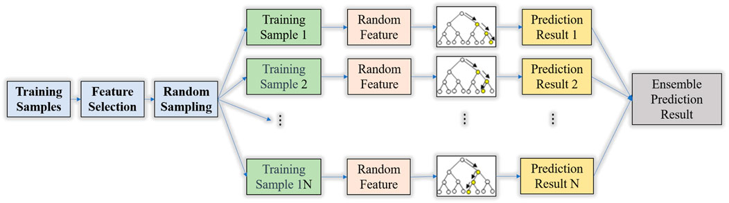
Figure 8. Schematic diagram of random forest model.

The core of the Random Forest lies in treating any individual decision tree as a base classifier. The samples are trained through decision trees to obtain different classification models h1(X)…… hk(X), and the final classification result is obtained through a voting mechanism. The formula for the final classification result is as follows:

$H\left(X\right)={\arg }_z^{\max }I(h_i\left(x\right)=Z$

In this context, “ $H\left(x\right)$” represents the classification output result of the Random Forest model, “ $h_i$”stands foran individual decision tree model, “Z” represents the output variable, and “ I(.)” is an indicator function. This indicates that the Random Forest adopts a majority voting decision method to determine the classification.

The study employs the training sample set from the research area (Figure 6; Table 2) to optimize four hyperparameters within the Random Forest model: max_depth, max_features, min_samples_split, and n_estimators. Utilizing the Bayesian optimization algorithm, it searches for the optimal hyperparameter values and outputs the values obtained during each iteration. By rounding these values to integers, the optimal hyperparameter values are determined as follows: {max_depth’: 13, ‘max_features’: 0.1, ‘min_samples_split’: 3, ‘n_estimators’: 166}. The refined hyperparameters for the Random Forest algorithm are illustrated in Table 3.

Table 3

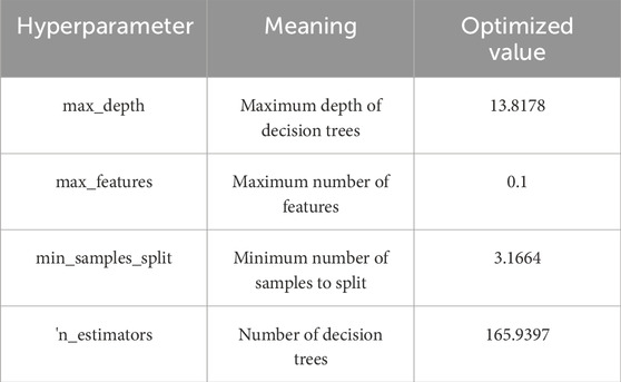
Table 3. Hyperparameters of the random forest model in the study area.

3.3.2 Constructing Convolutional Neural Network (CNN) model

The Convolutional Neural Network (CNN) is a type of deep learning model comprised of components such as convolutional layers, pooling layers, and fully connected layers. The convolutional layer serves as the core of CNN, detecting various features in images, such as edges, textures, or shapes, by applying convolutional operations on input data. These operations utilize learnable filters (also known as kernels) to scan the input data and generate feature maps. Pooling layers typically follow convolutional layers to reduce the size of feature maps and retain the most important information. They achieve this by downsampling the spatial dimensions of the feature maps, either by taking the maximum value (max pooling) or the average value (average pooling) within certain regions of the feature maps. This helps reduce the number of parameters and computational complexity while preserving crucial features. Fully connected layers are usually positioned at the end of CNN and are responsible for mapping the extracted features to the final output categories or predictions. These layers flatten the extracted features from the preceding layers and input them to fully connected neurons in the neural network to perform classification or regression tasks. As shown in Figure 9.

Figure 9

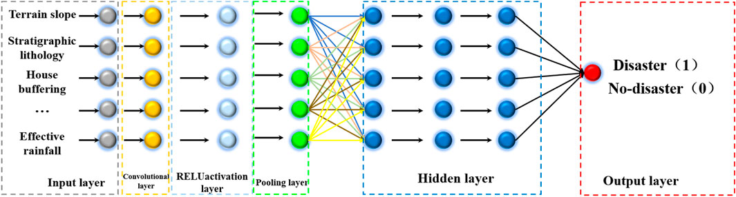
Figure 9. Schematic diagram of convolutional neural network (CNN) model.

This study utilized the training sample set from the research area (Figure 6; Table 2). The model architecture of the Convolutional Neural Network (CNN) comprises an input layer, an output layer, two convolutional layers, two max-pooling layers, a fully connected layer, and a dropout module aimed at preventing overfitting. Bayesian optimization algorithm was employed to search for partially optimal hyperparameters of the CNN model. This primarily involved determining the number of neurons in certain layers, activation functions for each layer, dropout rates for individual layer neurons, and the learning rate for model training. Specifically, the number of neurons in each layer was set to 512 x 1 for the initial convolutional layer and 32 x 1 for the second convolutional layer. The dropout rate for each layer was set to 0.1, with ReLU as the activation function for the first and second layers. The learning rate was fixed at 0.002. Other parameters were configured to the default settings of the CNN algorithm. The optimized hyperparameters of the Convolutional Neural Network are detailed in Table 4.

Table 4

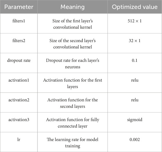
Table 4. Hyperparameters of the convolutional neural network model.

3.3.3 Multilayer Perceptron (MLP) model construction

Multilayer Perceptron (MLP) is a fundamental type of feedforward artificial neural network. It consists of multiple layers of neurons, including an input layer, at least one or more hidden layers, and an output layer (Hinton, 2006). In an MLP, each neuron is connected to all neurons in the previous layer, with each connection having an associated weight. Information flows from the input layer through the neurons and layers to the output layer. The presence of hidden layers allows MLP to learn and capture more complex patterns and features. MLP model are often trained using backpropagation algorithms, adjusting weights iteratively to minimize the error between predicted and actual outputs. This model applies to various machine learning tasks such as classification and regression. It is worth noting that MLP is commonly used for processing unstructured data like images, text, or time series data. While MLP is a simple and flexible model, it may suffer from overfitting or require more complex model structures to improve performance when dealing with complex problems.

This paper employs the training sample set of the research area (Figure 6; Table 2) to construct a Multilayer Perceptron (MLP) model, comprising one input layer, four hidden layers, and three dropout modules to mitigate overfitting. The optimization of the deep neural network model’s hyperparameters is achieved through the Bayesian optimization algorithm, considering factors such as the number of neurons in each layer, activation functions, dropout rates, and the learning rate. Specifically, the first layer has 64 neurons, the second and third layers each have 128 neurons, and the fourth layer has 54 neurons. The dropout rates for the neurons are 0.1, 0.43, and 0.35 for the first, second, and third layers, respectively. ReLU activation is used for the first layer, while sigmoid activation is applied to the subsequent layers, and the learning rate is set to 0.0001. Other parameters adhere to the default settings of the deep neural network algorithm. Table 5 presents the optimized hyperparameters for the Multilayer Perceptron model.

Table 5

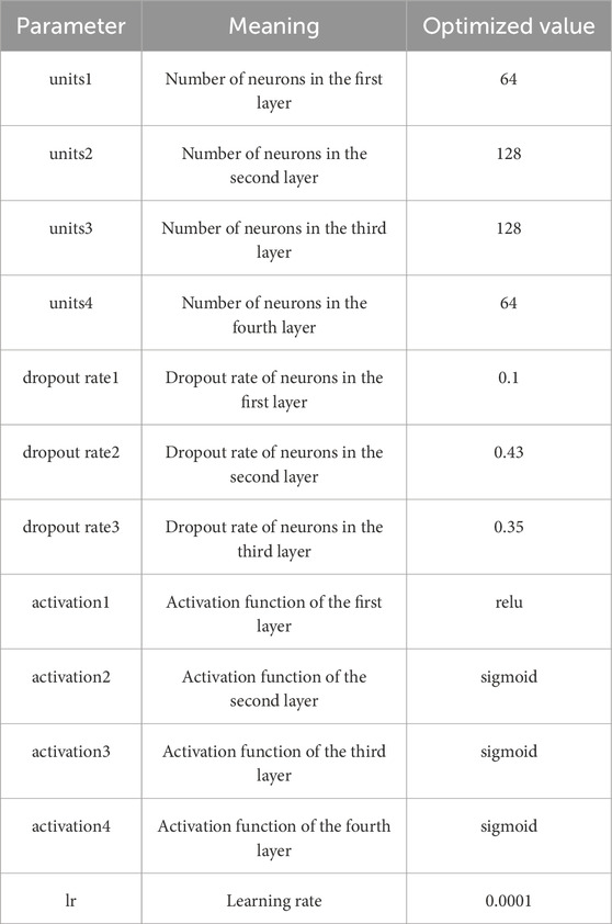
Table 5. Hyperparameters of the multilayer perceptron model.

3.3.4 Model optimization

When constructing artificial intelligence models, model training aims to enhance accuracy. Model accuracy relies not only on the learning algorithm’s performance but also on the selection of hyperparameters and features. Optimizing the model can also enhance accuracy, thus it is necessary to optimize certain parameters of each model. Presently, hyperparameter optimization methods can employ automatic tuning techniques. Automatic hyperparameter tuning methods mainly consist of random search, grid search, and Bayesian optimization algorithms. In contrast to grid search and random search, the Bayesian algorithm utilizes Gaussian processes, making full use of prior knowledge. Moreover, Bayesian optimization can attain the optimal solution and is more robust than random search. Consequently, this paper adopts the Bayesian optimization algorithm to adjust the model’s hyperparameters (Lee and Min, 2001).

Gaussian Process, also known as Gaussian distribution random process, can represent the distribution of functions. The characteristics of Gaussian distribution are determined by covariance and mean. By calculating the posterior probability of samples, the maximum posterior variance of the model output can be obtained. Generally, Gaussian processes require calculating the probability of each feature and multiplying them. However, due to the large number of feature factors, it is necessary to use a multivariate Gaussian regression model and establish the covariance matrix of features. Finally, the probability “p(χ) is calculated using all feature values.

$p\left(\chi \right)={\displaystyle \prod _j^n}p\left({\chi }_j;{\mu }_j;{\sigma }^2\right)={\displaystyle \prod _j^n}\frac{1}{\sqrt{2\mathrm{\pi }}{\sigma }_j}\exp \left\{-\left[\frac{{\left({\chi }_j-{\mu }_j\right)}^2}{2{\sigma }^2}\right]\right\}$

Average of all features:

${\mu }_j=\frac{1}{m}{\sum }_{i=1}^m{x}^i$

Covariance matrix:

$\sum =\frac{1}{m}{\displaystyle \sum _{i=1}^m}\left({\chi }^i-\mu \right){\left({\chi }^i-\mu \right)}^T=\frac{1}{m}{\left(X-\mu \right)}^T\left(X-\mu \right)$

Multivariate Gaussian distribution probability model:

$p\left(\chi \right)=\frac{1}{{2\mathrm{\pi }}^{\frac{\mathrm{\pi }}{2}}|{\left.\sum \right|}^{\frac{1}{2}}}\exp \left\{-\frac{1}{2}{\left(\chi -\mu \right)}^T\left.{\displaystyle \sum ^{-1}}\left(\chi -\mu \right)\right\}\right.$

During the process of searching for optimal values and optimizing hyperparameters, this process is a Gaussian process.

3.3.5 Model validation

To assess the performance of the model, two metrics, namely, the confusion matrix and ROC curve, were selected to evaluate the effectiveness of the regional landslide warning model. These metrics are used to measure the accuracy and generalization ability of the model, respectively.

(1) Confusion Matrix

The confusion matrix is a matrix used to evaluate the performance of classification models, providing an intuitive reflection of the model’s binary classification effectiveness. It categorizes the classification results into four scenarios based on the actual classes (true values) and predicted classes, namely, True Positive (TP), False Positive (FP), True Negative (TN), and False Negative (FN). The specific relationships between these four classification results are depicted in Table 6:

Table 6

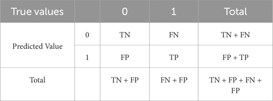
Table 6. Confusion matrix.

As shown in Table 6, TN represents the true negative value, which is the number of samples predicted and not experiencing landslides. FN represents the false negative value, indicating the number of samples predicted as not experiencing landslides but experiencing landslides. FP represents the false positive value, indicating the number of samples predicted as experiencing landslides but not. TP represents the true positive value, which is the number of samples predicted and experiencing landslides. Additionally, other classification metrics can be derived from the confusion matrix, including accuracy, true positive rate (TPR), sensitivity (recall), specificity, and negative predictive value (NPV), aiding in assessing the model’s performance. The formulas and meanings are presented in Table 7.

(2) ROC (Receiver Operating Characteristic) curve

Table 7

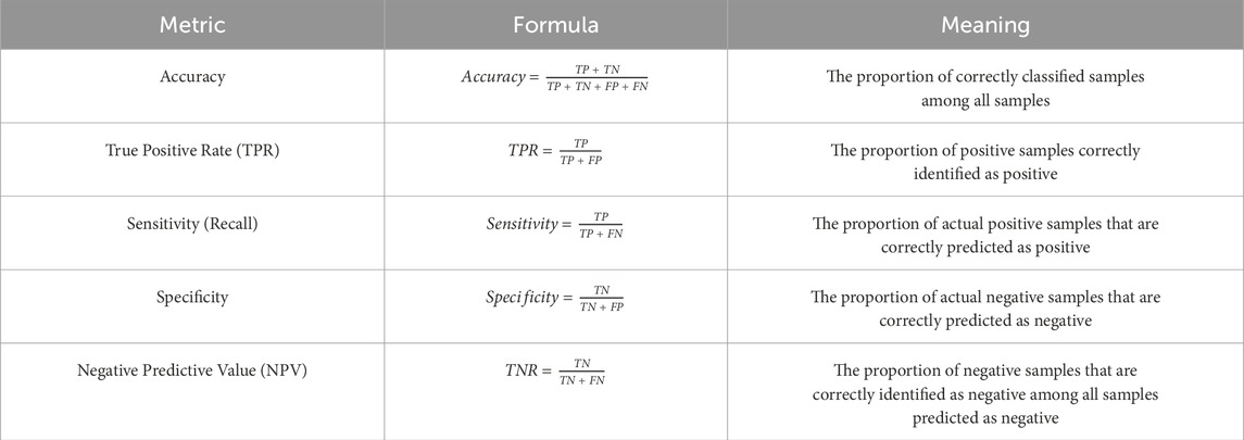
Table 7. Formulas and meanings of metrics.

The ROC curve is employed to comprehensively assess and evaluate the performance of the model. It is generated by plotting the true positive rate against the false positive rate at various thresholds. The value of AUC (Area Under the ROC Curve) represents the generalization ability of the landslide warning model, serving as an evaluation metric for model performance. AUC ranges from 0.5 to 1.0, with values closer to one indicating better model performance.

3.4 Model application

In practical applications, the pre-trained landslide warning models can be directly accessed using the LOAD function. These models have been previously trained, and saved, and can output the probability of landslide disasters occurring. By adhering to different warning strategies, the warning levels can be systematically determined and classified.

3.4.1 Model input and computation

Acquiring model input parameters by dividing the study area into grid cells of 2 km x 2 km. Each grid cell layer is then associated with 26 input feature parameters. These parameters include slope, terrain type, lithology, annual rainfall, vegetation type, distance to watercourses, distance to roads, distance to buildings, population density, and historical disaster points, which are derived from geological environmental input features trained by the model. The remaining 16 input feature parameters, such as rainfall for the current day, rainfall for the previous 1 day, rainfall for the previous 2 days, and so forth up to rainfall for the previous 15 days, are computed based on the specific time of the day for which the warning calculation is performed. Ultimately, this process generates input data files for each grid cell. These input data files are then fed into the three machine-learning landslide warning models for computation, yielding the output of landslide hazard probabilities within each grid cell.

3.4.2 Warning strategy

Based on the probabilities of landslides occurring in each grid cell as output by the model, the final warning level is determined according to the model’s output strategy. This paper proposes two warning strategies: binary warning strategy and multiclass warning strategy.

(1) Binary Warning Strategy

The binary warning strategy categorizes the final warning level into two classes based on the probabilities of landslides occurring in each grid cell as output by the model: no warning and warning. We set the threshold for classification at 50% and use this threshold to determine the landslide warning level. When the probability of landslides in each grid cell output by the model is below the 50% threshold, the warning level is classified as “no warning,” indicating a low risk of geological disaster occurrence. Conversely, when the probability of landslides in each grid cell output by the model is above the 50% threshold, the warning level is classified as “warning,” still indicating a high risk of geological disaster occurrence (Table 8).

(2) Multiple Classification Warning Strategy

Table 8

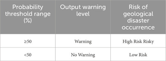
Table 8. Binary warning strategy based on machine learning landslide warning models.

The multiple classification warning strategy divides the final warning level into several categories based on the landslide occurrence probability output by the model for each grid cell. This study refers to the industry standard geological disaster meteorological risk warning regulations, using thresholds of 20%, 40%, 60%, and 80% to categorize the warning levels into no warning, yellow warning, orange warning, and red warning. Specifically, when the output probability is below 40%, the warning level is “no warning,” indicating a relatively low risk of geological disaster occurrence. When the output probability falls within the range of 40%–60%, the warning level is “yellow warning,” suggesting a higher risk of geological disaster occurrence. For output probabilities between 60% and 80%, the warning level is “orange warning,” indicating a high risk of geological disaster occurrence. If the output probability exceeds 80%, the warning level is “red warning,” indicating a very high risk of geological disaster occurrence (Table 9).

Table 9

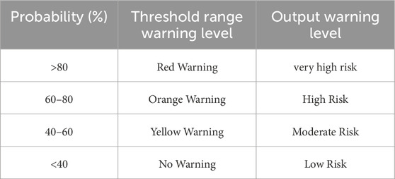
Table 9. Multi-class warning strategy based on machine learning landslide warning model.

4 Results and comparative analysis of three warning models

4.1 Model validation results

(1) Confusion Matrix Results

According to the confusion matrix output results of the three models (Table 10), it can be observed that when thresholds are set to 0.25, 0.5, and 0.75 respectively, the accuracy of the Random Forest model is 0.930, 0.953, and 0.957, the accuracy of the Convolutional Neural Network (CNN) model is 0.945, 0.947, and 0.948, and the accuracy of the Multilayer Perceptron (MLP) model is 0.930, 0.937, and 0.953. According to the ROC results of the three models (Figure 10), the AUC value of the Random Forest model is 0.955, the AUC value of the CNN model is 0.940, and the AUC value of the MLP model is 0.930. The test metrics of the three models are very close, demonstrating good generalization ability and accuracy of all three models, proving their reliability. Comparatively, among the three models, the Random Forest model exhibits the highest accuracy (0.957) and the highest AUC value (0.955).

(2) ROC Results

Table 10

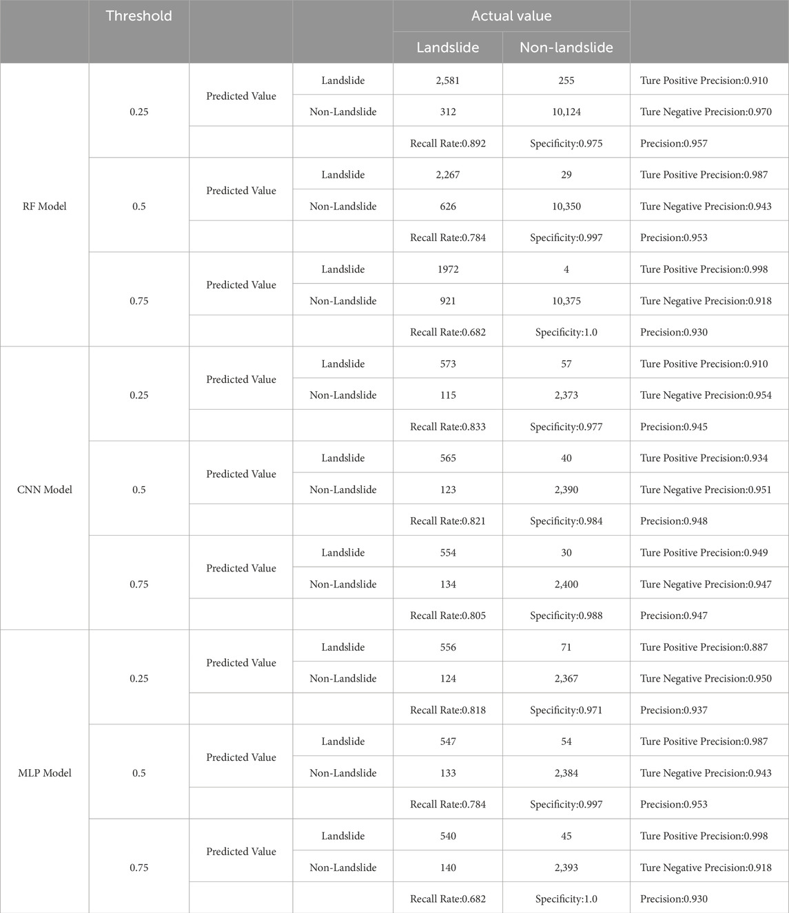
Table 10. Confusion matrix results of three warning models.

Figure 10

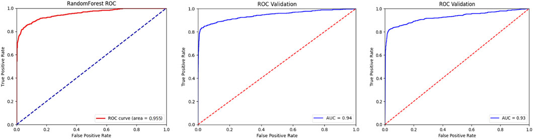
Figure 10. ROC Curve Results (A): RF Model; (B) CNN Model; (C) MLP Model).

4.2 The effectiveness of model application in early warning

As an example, let’s consider 5 August 2021, and apply the model input, model computation, and early warning strategy outlined in Section 2.4. We’ll generate the risk warning levels for geological disasters according to both the binary and multiclass warning strategies. The results for the binary warning strategy are shown in Figure 11, while the results for the multiclass warning strategy are shown in Figure 12.

Figure 11

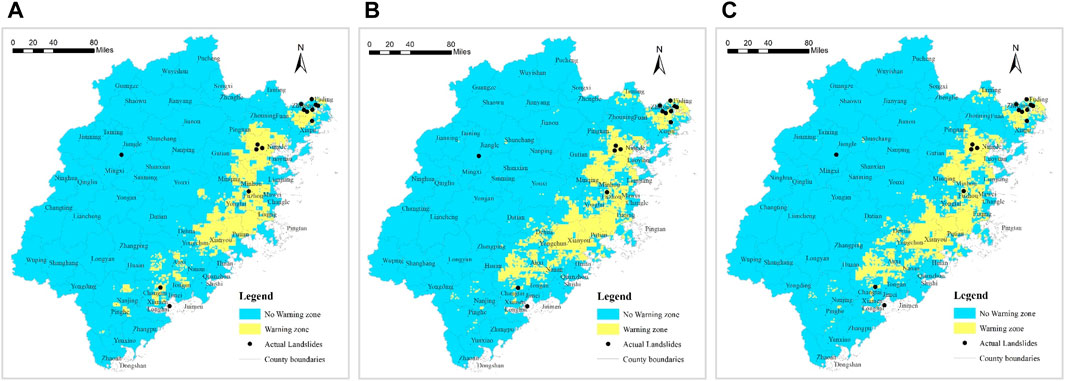
Figure 11. Verification Results of Binary Warning Strategy Instance (A): RF Warning Model; (B) CNN Warning Model; (C) MLP Warning Model).

Figure 12

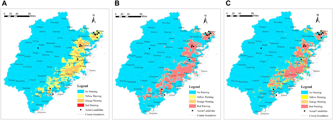
Figure 12. Multiclass Warning Strategy Validation Results (A): RF Warning Model; (B) CNN Warning Model; (C) MLP Warning Model).

We’ll then collect and organize the actual landslide disaster occurrences in the study area on 5 August 2021 (14 newly occurred landslides). By mapping the coordinates of the actual landslide points onto the warning result maps (Figures 11, 12), we’ll validate the effectiveness of the model’s practical application.

From Figure 11 and Table 11, it is evident that in the results of the binary warning strategy, among all 14 newly occurred landslide points, 13 fall within the “Warning” level range of the Random Forest (RF) model (Figure 11A), achieving a prediction hit rate of 92.9%; 13 newly occurred landslide points fall within the “Warning” level range of the Convolutional Neural Network (CNN) model (Figure 11B), with a prediction hit rate of 92.9%; and 12 newly occurred landslide points fall within the “Warning” level range of the Multilayer Perceptron (MLP) model (Figure 11C), achieving a prediction hit rate of 85.7%.

Table 11

Table 11. Comparison of the actual application effectiveness of three models in warning.

From Figure 13 and Table 11, in the results of the multiclass warning strategy, the Random Forest model’s warning results (Figure 12A) show that among all 14 newly occurred landslide points, 13 (92.9%) fall within the Random Forest model’s warning zone, with approximately half falling into the “Yellow Warning” and “Orange Warning” zones and no newly occurred landslide points fall into the “Red Warning” zone. The CNN warning model results (Figure 12B) indicate that among all 14 newly occurred landslide points, 13 (92.9%) fall within the CNN model’s warning zone, with no newly occurred landslide points falling into the “Yellow Warning” zone, and approximately 86% fall into the “Red Warning” zone. The MLP warning model results (Figure 12C) show that among all 14 newly occurred landslide points, 12 (85.8%) fall within the MLP model’s warning zone, with no newly occurred landslide points falling into the “Orange Warning” zone, and 71.4% fall into the “Red Warning” zone.

Figure 13

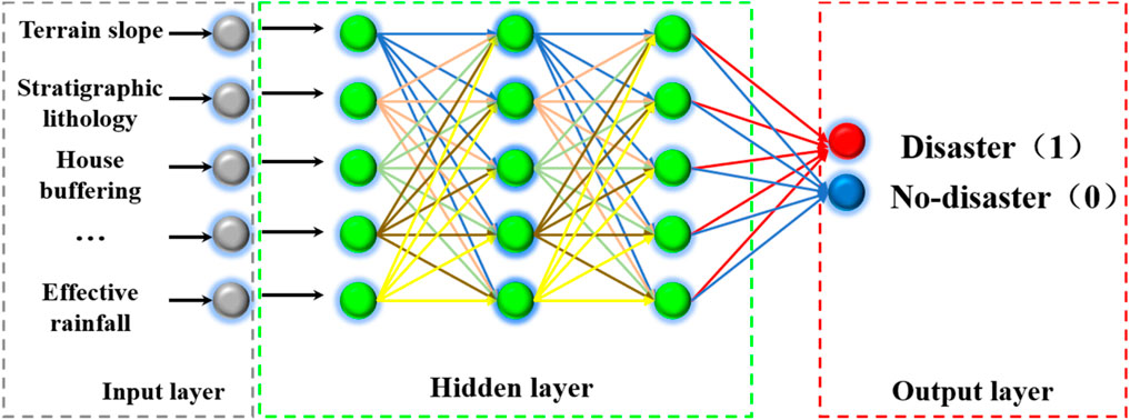
Figure 13. Schematic diagram of multilayer perceptron (MLP) model.

Comparative analysis shows that the Random Forest warning model not only performs excellently in accuracy but also exhibits outstanding performance in multi-level hierarchical warning. The warning zones of different levels are distributed more evenly, indicating that the Random Forest model is more suitable for multi-level warnings. The CNN and MLP warning models demonstrate good accuracy, but they perform inadequately in hierarchical warning, with their output results tending toward the two extremes of 0 and 1. Consequently, the majority of the warning zones in the output results of these two models are in the “Red Warning” zone, indicating their limitations in hierarchical warning applications.

4.3 Analysis of results

In the model training and evaluation phase, we employed three machine learning algorithms: Random Forest (RF), Multi-Layer Perceptron (MLP), and Convolutional Neural Network (CNN) for learning, training, and validating the landslide disaster warning models. The dataset was divided into training and testing sets in a 4:1 ratio, and a Bayesian optimization algorithm was used to optimize the model’s hyperparameters. The reliability of the models was thoroughly tested on the testing set using confusion matrices and ROC curves. Evaluation results showed that the accuracy of the warning model based on the Random Forest algorithm ranged from 0.930 to 0.957, with an AUC value of 0.955; for the Convolutional Neural Network-based warning model, the accuracy ranged from 0.945 to 0.948, with an AUC value of 0.940; and for the Multi-Layer Perceptron-based warning model, the accuracy ranged from 0.930 to 0.953, with an AUC value of 0.930. The results indicate that the accuracy of the three models’ testing metrics is comparable, but the Random Forest algorithm demonstrates a clear advantage in terms of AUC value. All three models exhibit good generalization ability and precision. In terms of model application, methods for obtaining and importing input feature parameters in practical warning scenarios are proposed. Two standardized warning model output feature strategies are suggested: binary classification warning and multi-classification warning. In the binary classification warning strategy, a threshold of 50% is used for the output probability, dividing the warning results into “no warning” and “warning” categories. In the multi-classification warning strategy, thresholds of 40%, 60%, and 80% are utilized, categorizing the warning results into “no warning,” “yellow warning,” “orange warning,” and “red warning” classes. Taking the widespread landslide disasters triggered by heavy rainfall in Fujian Province, China on 5 August 2021, as an example, the practical application of the models in real scenarios was demonstrated. Results revealed that using the binary classification warning strategy, out of the 14 landslide disasters that occurred on 5 August 2021, 13 landslides (accounting for 92.9% of the total) fell within the “warning” areas predicted by the Random Forest and Convolutional Neural Network (CNN) warning models, while 12 landslides (85.7% of the total) fell within the “warning” areas predicted by the Multi-Layer Perceptron (MLP) warning model. This demonstrates the excellent performance of the three warning models in the binary classification warning strategy. When employing the multi-classification warning strategy, within the output results of the Random Forest warning model, seven landslides (50.0% of the total) fell into the “yellow warning” zone, six landslides (42.9% of the total) fell into the “orange warning” zone, and one landslide (7.1% of the total) fell into the “no warning” zone. In the output results of the CNN warning model, 12 landslides (85.8% of the total) fell into the “red warning” zone, one landslide (7.1% of the total) fell into the “orange warning” zone, and one landslide (7.1% of the total) fell into the “no warning” zone. In the output results of the MLP warning model, 10 landslides (71.4% of the total) fell into the “red warning” zone, two landslides (14.3% of the total) fell into the “orange warning” zone, and two landslide (14.3% of the total) fell into the “no warning” zone. Comparative analysis indicates that the Random Forest warning model not only demonstrates excellent accuracy but also performs remarkably well in multi-classification hierarchical warning. The CNN and MLP warning models exhibit good accuracy in warning but show limitations in hierarchical warning effectiveness.

5 Discussion

This study uses three machine learning algorithms—Random Forest (RF), Multi-Layer Perceptron (MLP), and Convolutional Neural Network (CNN)—to provide a broader assessment of model performance. The use of multiple algorithms allows for a comparison of different methods, identifying their respective strengths and weaknesses. Previous research typically focused on a single algorithm, limiting the scope of comparative analysis (Hastie et al., 2009). Implementing both binary and multiclass classification strategies enhances the versatility and applicability of the warning models. By categorizing warning results into different risk levels, stakeholders can better prioritize and manage resources. This dual-strategy approach is relatively unique and adds depth to the predictive capability of the models (Breiman, 2001). The models demonstrated strong generalization ability and high accuracy during the testing phase, particularly the Random Forest algorithm, which achieved the highest AUC value. This robustness is crucial for the practical application of landslide prediction, where model reliability is key (Zhou et al., 2020). Previous research on landslide warning models often used single algorithms and simple classification strategies. For example, studies by Dou et al. (2020) and Hong et al. (2016b) mainly used logistic regression and support vector machines, focusing on binary classification. This study employs multiple algorithms and classification strategies, providing a more detailed and comprehensive analysis. It demonstrates the relative advantages of different methods in various contexts. Liu et al. (2022) conducted a study on landslide disaster early-warning models using six machine learning algorithms. Among them, the Random Forest model performed the best, with the highest generalization ability (AUC = 0.955) and no overfitting. The Artificial Neural Network model followed with an AUC of 0.935, then the Nearest Neighbor model, Logistic Regression model, and Support Vector Machine model with AUCs of 0.924, 0.922, and 0.920, respectively. The Decision Tree performed the worst, with an AUC value of 0.904 and an accuracy of 0.937. In comparison, the AUC values of the three early-warning models in this paper are 0.955 for the Random Forest algorithm, 0.940 for the Convolutional Neural Network-based warning model, and 0.930 for the Multi-Layer Perceptron-based warning model. The overall AUC value differences are relatively small, and the values are higher, indicating that the early-warning models established using these three algorithms are more stable.

The Random Forest algorithm typically yields excellent predictive results, even when dealing with complex or high-dimensional datasets. It can effectively handle large datasets and exhibits good robustness towards missing data. Random Forest can also fit nonlinear relationships in data quite well. However, it may perform poorly when dealing with high-dimensional sparse data. CNN excels in processing data with grid-like structures such as images and speech because they can effectively capture local features. Through mechanisms like weight sharing and local connections, CNN reduces the number of parameters, thereby improving the model’s training efficiency and generalization ability. However, CNN may not perform well when dealing with sequential data or non-grid structured data, as their architecture assumes input data have a grid-like structure. CNN requires a large amount of data for training to avoid overfitting issues. MLP can adapt to various types of data, including structured and unstructured data. Their model structure is relatively simple, making them easy to understand and implement. However, for high-dimensional or large-scale data, MLP may not be efficient enough as they typically require a large number of parameters to learn complex patterns. However, the dataset established in this study features characteristics such as being large and low-dimensional, making it suitable for the application conditions of Random Forests, CNN, and MLP. This is also why these three models perform well in predicting landslide outcomes.

Although the three models show small numerical differences in validation metrics (such as AUC values and accuracy), these minor differences can lead to significant differences in practical applications. Specifically, we observed the following points:(1) Geographical Distribution Differences: In practical applications, different models show significant differences in the warning areas on geographical distribution maps. Taking the landslide disasters in Fujian Province on 5 August 2021, as an example, although the RF and CNN models are very close in accuracy and AUC values, they exhibit significant differences in the predicted warning areas. The RF model tends to issue warnings in medium-risk areas, while the CNN model issues more warnings in high-risk areas. (2)Reason Analysis: This difference mainly stems from the sensitivity of the models to input features. The RF model performs well in capturing potential risk points due to its ability to handle highly nonlinear relationships in the data. On the other hand, the CNN model effectively captures spatial features through its convolutional layers, leading to more accurate predictions in high-risk areas. (3)Impact Analysis: These small differences in metrics can lead to significant differences in practical applications. For example, the RF model predicts more warnings in “yellow warning” and “orange warning” areas, which is crucial for disaster prevention in medium-risk regions. The high accuracy of the CNN model in “red warning” areas means better preparedness in high-risk regions. The MLP model also provides higher warnings in some low-risk areas, offering additional references for overall risk management. Through the above analysis, we further illustrate that although the three models have small differences in validation metrics, these differences can translate into significant differences in practical applications. This part of the discussion not only highlights the applicability of the models in different scenarios but also provides valuable insights for practical disaster warning work.

The article employs two warning strategies. The binary warning strategy categorizes the final warning level into two classes: no warning and warning, corresponding to low and high predicted geological disaster risks, respectively. The binary classification strategy is simple and intuitive, well-suited for scenarios requiring direct disaster prediction and emphasizing rapid decision-making. Involving only two categories contributes to high computational efficiency and straightforward decision-making, facilitating swift responses to emergencies. The multiclass warning strategy classifies the final warning level into multiple levels: no warning, yellow warning, orange warning, and red warning. These graded warnings (red, orange, yellow) correspond to very high, high, and relatively high risks of geological disasters. The multiclassification strategy distinguishes between various types or different levels of disaster states, providing more detailed and refined predictive outcomes. This strategy is suitable for regions and situations characterized by diverse types of disasters and higher complexity. It enables more accurate predictions for each potential disaster state and corresponding emergency response measures, thereby enhancing disaster preparedness capabilities. The advantages and disadvantages of these strategies are summarized in the following Table 12.

Table 12

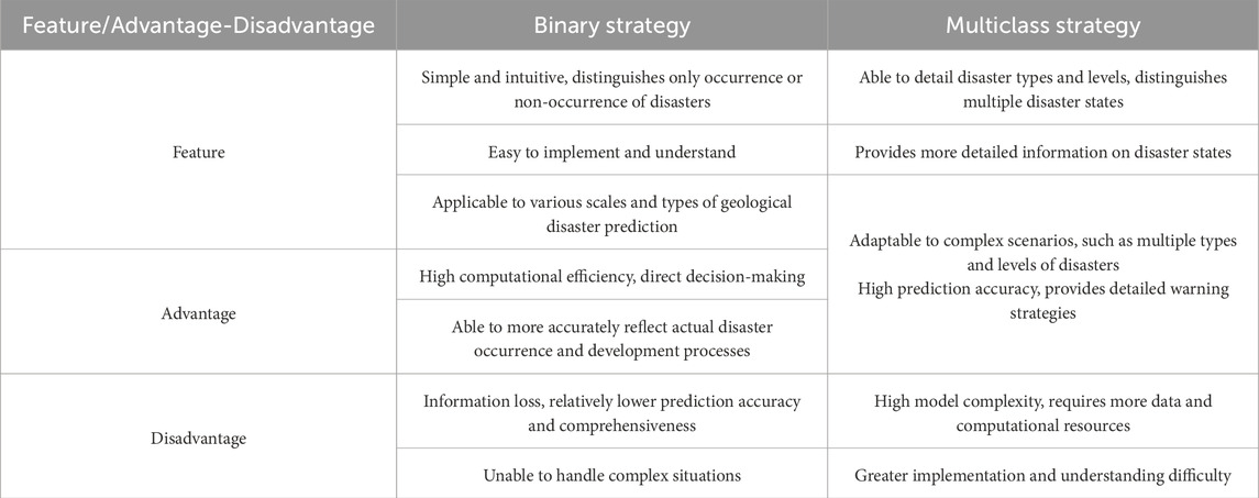
Table 12. The binary strategy and multiclass strategy.

The application of these models in practical landslide prediction demonstrates their potential. However, limitations such as handling high-dimensional data and the data requirements of CNNs need to be addressed in future research. To further improve the robustness and applicability of landslide warning models, future studies should consider integrating hybrid models that combine the strengths of various algorithms. Additionally, exploring advanced machine learning techniques such as ensemble learning, transfer learning, and unsupervised learning can enhance model performance. Subsequent optimization of input features and validation of models using more diverse datasets will also be beneficial.

6 Conclusion

This study presents a comprehensive approach to constructing regional landslide warning models utilizing machine learning, demonstrated within the context of Fujian Province, China. The outlined four-step process includes data integration and cleaning, construction of training sample sets, machine learning model training and validation, and practical model application. Employing Random Forest (RF), Convolutional Neural Network (CNN), and Multilayer Perceptron (MLP) algorithms, the research showcases the effectiveness of these models in predicting rainfall-induced landslides.

(1) The dataset utilized for model development comprises 15,589 samples, incorporating 10 geological environmental condition factors and 16 rainfall-induced features. This diverse dataset provides a robust foundation for training and testing the models.

(2) The training and evaluation phase highlights the performance of RF, CNN, and MLP algorithms, revealing comparable accuracy metrics. The RF algorithm notably excels with a higher AUC value, indicating superior predictive capability.

(3) In practical model application, two standardized warning strategies are proposed: binary classification and multi-classification. The binary classification strategy distinguishes between “no warning” and “warning” categories based on a 50% threshold, while the multi-classification strategy offers nuanced warnings, dividing predictions into “no warning,” “yellow warning,” “orange warning,” and “red warning” classes using varying thresholds.

(4) Real-world application of the models during the 5 August 2021 landslide disasters in Fujian Province demonstrates their efficacy. In the binary classification strategy, the models successfully predicted the majority of landslide occurrences. In the multi-classification approach, the RF model exhibits superior hierarchical warning effectiveness compared to CNN and MLP models.

In summary, this research significantly contributes to advancing landslide disaster warning models by providing insights into model construction, evaluation, and practical application. Further refinement and validation of these models are anticipated through continued data accumulation and real-world verification.

The paper only conducts statistical analysis on the relationship between various factors and landslide occurrences, lacking sufficient insight into the mechanism and causes of landslides. In the future, it is necessary to employ more rational and complex nonlinear methods for research. Although the sample set used in this study achieves a balance between positive and negative samples through the SMOTE algorithm, the generated synthetic samples are obtained through linear interpolation, which may introduce errors compared to the actual local conditions. Therefore, in future sample dataset construction, it is essential to select positive and negative samples proportionally. The warning methods studied in the paper have implications for broader application. Currently, they are only used in Fujian Province, but they could be applied to other regions in the future. By collecting different disaster-causing factors to construct sample sets, a regional geological disaster meteorological warning model could be developed, thus further verifying its applicability.

Data availability statement

The data analyzed in this study is subject to the following licenses/restrictions: Departmental reasons cannot be fully shared. Requests to access these datasets should be directed to lyanhui@mail.cgs.gov.cn.

Author contributions

YL: Conceptualization, Formal Analysis, Funding acquisition, Investigation, Methodology, Project administration, Resources, Supervision, Validation, Writing–original draft, Writing–review and editing, Data curation, Software, Visualization. SM: Data curation, Investigation, Methodology, Resources, Writing–original draft, Writing–review and editing. LD: Data curation, Formal Analysis, Investigation, Methodology, Resources, Software, Writing–original draft. RX: Conceptualization, Investigation, Project administration, Resources, Supervision, Writing–original draft. JH: Data curation, Investigation, Resources, Validation, Writing–original draft. PZ: Conceptualization, Funding acquisition, Investigation, Project administration, Resources, Supervision, Validation, Writing–original draft, Methodology, Writing–review and editing.

Funding

The author(s) declare that financial support was received for the research, authorship, and/or publication of this article. This research was financially supported by the National Key Research and Development Program of China (2023YFC3007205) and the National Natural Science Foundation of China(42077440; 41202217).

Acknowledgments

Thanks for the China Institute of Geo-Environment Monitoring and the Fujian Provincial Geological Environmental Monitoring Center for providing the historical landslide records data. We also appreciate the Fujian Meteorological Bureau and the Fujian Water Resources Department for providing the rainfall data.

Conflict of interest

Author LD was employed by Power China Beijing Engineering Corporation Limited.

The remaining authors declare that the research was conducted in the absence of any commercial or financial relationships that could be construed as a potential conflict of interest.

Publisher’s note

All claims expressed in this article are solely those of the authors and do not necessarily represent those of their affiliated organizations, or those of the publisher, the editors and the reviewers. Any product that may be evaluated in this article, or claim that may be made by its manufacturer, is not guaranteed or endorsed by the publisher.

References

Abraham, M. T., Satyam, N., Rosi, A., Pradhan, B., and Segoni, S. (2020). The selection of rain gauges and rainfall parameters in estimating intensity-duration thresholds for landslide occurrence: case study from Wayanad (India). Water 12 (4), 1000. doi:10.3390/w12041000

CrossRef Full Text | Google Scholar

Ado, M., Amitab, K., Maji, A. K., Jasińska, E., Gono, R., Leonowicz, Z., et al. (2022). Landslide susceptibility mapping using machine learning: a literature survey. Remote Sens. 14 (13), 3029. doi:10.3390/rs14133029

CrossRef Full Text | Google Scholar

Aleotti, P. (2004). A warning system for rainfall-induced shallow failures. Eng. Geol. 73 (3-4), 247–265. doi:10.1016/j.enggeo.2004.01.007

CrossRef Full Text | Google Scholar

Au, S. W. C. (1998). Rain-induced slope instability in Hong Kong. Eng. Geol. 51 (1), 1–36. doi:10.1016/s0013-7952(98)00038-6

CrossRef Full Text | Google Scholar

Baum, R. L., and Godt, J. W. (2010). Early warning of rainfall-induced shallow landslides and debris flows in the USA. Landslides 7, 259–272. doi:10.1007/s10346-009-0177-0

CrossRef Full Text | Google Scholar

Breiman, L. (2001). Random forests. Mach. Learn. 45 (1), 5–32. doi:10.1023/a:1010933404324

CrossRef Full Text | Google Scholar

Caine, N. (1980). The rainfall intensity-duration control of shallow landslides and debris flows. Geogr. Ann. Ser. A, Phys. Geogr. 62 (1-2), 23–27. doi:10.2307/520449

CrossRef Full Text | Google Scholar

Cannon, S. H. (1985). Rainfall conditions for abundant debris avalanches, San Francisco Bay region, California. Geology 38, 267–272.

Google Scholar

Chen, W., Xie, X., Wang, J., Pradhan, B., Hong, H., Bui, D. T., et al. (2017). A comparative study of logistic model tree, random forest, and classification and regression tree models for spatial prediction of landslide susceptibility. Catena 151, 147–160. doi:10.1016/j.catena.2016.11.032

CrossRef Full Text | Google Scholar

Ding, G., Wang, Y., Mao, J., et al. (2017). Study on rainfall warning thresholds in debris flow prone areas of beijing. Hydrogeology Eng. Geol. 44 (3), 136–142. (in Chinese). doi:10.16030/j.cnki.issn.1000-3665.2017.03.20

CrossRef Full Text | Google Scholar

Dong, L., Liu, Y., Huang, J., et al. (2024). An early prediction model of regional landslide disasters in Fujian Province based on convolutional neural network. Hydrogeology Eng. Geol. 51 (1), 145–153. doi:10.16030/j.cnki.issn.1000-3665.202211018

CrossRef Full Text | Google Scholar

Dou, J., Yamagishi, H., Pourghasemi, H. R., Yunus, A. P., Song, X., Xu, Y., et al. (2015). An integrated artificial neural network model for the landslide susceptibility assessment of Osado Island, Japan. Nat. Hazards 78, 1749–1776. doi:10.1007/s11069-015-1799-2

CrossRef Full Text | Google Scholar

Dou, J., Yunus, A. P., Merghadi, A., Shirzadi, A., Nguyen, H., and Hussain, Y. (2020). Different sampling strategies for predicting landslide susceptibilities are deemed less consequential with deep learning. Sci. Total Environ. 720, 137320. doi:10.1016/j.scitotenv.2020.137320

PubMed Abstract | CrossRef Full Text | Google Scholar

Froude, M. J., and Petley, D. N. (2018). Global fatal landslide occurrence from 2004 to 2016. Nat. Hazards Earth Syst. Sci. 18 (8), 2161–2181. doi:10.5194/nhess-18-2161-2018

CrossRef Full Text | Google Scholar

Gatto, A., Clò, S., Martellozzo, F., and Segoni, S. (2023). Tracking a decade of hydrogeological emergencies in Italian municipalities. Data 8 (10), 151. doi:10.3390/data8100151

CrossRef Full Text | Google Scholar

Goetz, J. N., Brenning, A., Petschko, H., and Leopold, P. (2015). Evaluating machine learning and statistical prediction techniques for landslide susceptibility modeling. Comput. geosciences 81, 1–11. doi:10.1016/j.cageo.2015.04.007

CrossRef Full Text | Google Scholar

Hastie, T., Tibshirani, R., and Friedman, J. (2009). The elements of statistical learning: data mining, inference, and prediction. Germany: Springer.

Google Scholar

Hong, H., Pourghasemi, H. R., and Pourtaghi, Z. S. (2016a). Landslide susceptibility assessment in Lianhua County (China): a comparison between a random forest data mining technique and bivariate and multivariate statistical models. Geomorphology 259, 105–118. doi:10.1016/j.geomorph.2016.02.012

CrossRef Full Text | Google Scholar

Hong, H., Pradhan, B., Jebur, M. N., Bui, D. T., Xu, C., and Akgun, A. (2016b). Spatial prediction of landslide hazard at the Luxi area (China) using support vector machines. Environ. Earth Sci. 75, 1–14. doi:10.1007/s12665-015-4866-9

CrossRef Full Text | Google Scholar

Khan, S., Kirschbaum, D. B., Stanley, T. A., Amatya, P. M., and Emberson, R. A. (2022). Global landslide forecasting system for hazard assessment and situational awareness. Front. Earth Sci. 10, 878996. doi:10.3389/feart.2022.878996

CrossRef Full Text | Google Scholar

Krøgli, I. K., Devoli, G., Colleuille, H., Boje, S., Sund, M., and Engen, I. K. (2018). The Norwegian forecasting and warning service for rainfall-and snowmelt-induced landslides. Nat. hazards earth Syst. Sci. 18 (5), 1427–1450. doi:10.5194/nhess-18-1427-2018

CrossRef Full Text | Google Scholar

Lee, J. J., Song, M. S., Yun, H. S., and Yum, S. G. (2022). Dynamic landslide susceptibility analysis that combines rainfall period, accumulated rainfall, and geospatial information. Sci. Rep. 12 (1), 18429. doi:10.1038/s41598-022-21795-z

PubMed Abstract | CrossRef Full Text | Google Scholar

Lima, P., Steger, S., Glade, T., and Murillo-García, F. G. (2022). Literature review and bibliometric analysis on data-driven assessment of landslide susceptibility. J. Mt. Sci. 19 (6), 1670–1698. doi:10.1007/s11629-021-7254-9

CrossRef Full Text | Google Scholar

Liu, C., Liu, Y., Wen, M., et al. (2015). Practice of geological disaster meteorological warning in China: 2003-2012. J. Geol. Hazards Prev. Res. 26 (1), 1–8. (in Chinese). doi:10.16031/j.cnki.issn.1003-8035.2015.01.001

CrossRef Full Text | Google Scholar

Liu, Y., Huang, J., Xiao, R., Ma, S., and Zhou, P. (2022). Research on a regional landslide early-warning model based on machine learning—a case study of Fujian Province, China. Forests 13 (12), 2182.doi:10.3390/f13122182

CrossRef Full Text | Google Scholar

Liu, Y., Yin, K., and Liu, B. (2010). Application of logistic regression and artificial neural network models in spatial prediction of landslide disasters. Hydrogeology Eng. Geol. (5), 92–96. (in Chinese). doi:10.16030/j.cnki.issn.1000-3665.2010.05.015

CrossRef Full Text | Google Scholar

Luti, T., Segoni, S., Catani, F., Munafò, M., and Casagli, N. (2020). Integration of remotely sensed soil sealing data in landslide susceptibility mapping. Remote Sens. 12 (9), 1486. doi:10.3390/rs12091486

CrossRef Full Text | Google Scholar

Marjanovic, M., Bajat, B., and Kovacevic, M. (2009). Landslide susceptibility assessment with machine learning algorithms[C]//2009 international conference on intelligent networking and collaborative systems. IEEE, 273–278. doi:10.1109/INCOS.2009.25

CrossRef Full Text | Google Scholar

Micheletti, N., Foresti, L., Robert, S., Leuenberger, M., Pedrazzini, A., Jaboyedoff, M., et al. (2014). Machine learning feature selection methods for landslide susceptibility mapping. Math. Geosci. 46, 33–57. doi:10.1007/s11004-013-9511-0

CrossRef Full Text | Google Scholar

Ministry of Natural Resources, Geological Hazard Technical Guidance Center (2019). National geological disaster bulletin (2019) [R]. Beijing: Ministry of natural Resources, geological hazard technical guidance center.

Google Scholar

Mulyana, A. R., Sutanto, S. J., Hidayat, R., et al. (2019). Capability of Indonesian landslide early warning system to detect landslide occurrences few days in advance. Geophys. Res. Abstr. 21.

Google Scholar

Nocentini, N., Rosi, A., Segoni, S., and Fanti, R. (2023). Towards landslide space-time forecasting through machine learning: the influence of rainfall parameters and model setting. Front. Earth Sci. 11, 1152130. doi:10.3389/feart.2023.1152130

CrossRef Full Text | Google Scholar

Pennington, C., Freeborough, K., Dashwood, C., Dijkstra, T., and Lawrie, K. (2015). The national landslide database of great britain: acquisition, communication and the role of social media. Geomorphology 249, 44–51. doi:10.1016/j.geomorph.2015.03.013

CrossRef Full Text | Google Scholar

Peruccacci, S., Brunetti, M. T., Gariano, S. L., Melillo, M., Rossi, M., and Guzzetti, F. (2017). Rainfall thresholds for possible landslide occurrence in Italy. Geomorphology 290, 39–57. doi:10.1016/j.geomorph.2017.03.031

CrossRef Full Text | Google Scholar

Ponziani, F., Berni, N., Stelluti, M., Zauri, R., Pandolfo, C., Brocca, L., et al. (2013). LANDWARN: an operative early warning system for landslides forecasting based on rainfall thresholds and soil moisture. Landslide Sci. Pract. Volume 2 Early Warn. Instrum. Monit., 627–634. doi:10.1007/978-3-642-31445-2_82

CrossRef Full Text | Google Scholar

Reichenbach, P., Rossi, M., Malamud, B. D., Mihir, M., and Guzzetti, F. (2018). A review of statistically-based landslide susceptibility models. Earth-science Rev. 180, 60–91. doi:10.1016/j.earscirev.2018.03.001

CrossRef Full Text | Google Scholar

Ren, T., Gao, L., and Gong, W. (2024). An ensemble of dynamic rainfall index and machine learning method for spatiotemporal landslide susceptibility modeling. Landslides 21 (2), 257–273. doi:10.1007/s10346-023-02152-1

CrossRef Full Text | Google Scholar

Sameen, M. I., Pradhan, B., and Lee, S. (2020). Application of convolutional neural networks featuring Bayesian optimization for landslide susceptibility assessment. Catena 186, 104249. doi:10.1016/j.catena.2019.104249

CrossRef Full Text | Google Scholar

Sun, D., Gu, Q., Wen, H., Shi, S., Mi, C., and Zhang, F. (2022). A hybrid landslide warning model coupling susceptibility zoning and precipitation. Forests 13 (6), 827. doi:10.3390/f13060827

CrossRef Full Text | Google Scholar

Thai Pham, B., Shirzadi, A., Shahabi, H., Omidvar, E., Singh, S. K., Sahana, M., et al. (2019). Landslide susceptibility assessment by novel hybrid machine learning algorithms. Sustainability 11 (16), 4386. doi:10.3390/su11164386

CrossRef Full Text | Google Scholar

Tien Bui, D., Tuan, T. A., Hoang, N. D., Thanh, N. Q., Nguyen, D. B., Van Liem, N., et al. (2017). Spatial prediction of rainfall-induced landslides for the Lao Cai area (Vietnam) using a hybrid intelligent approach of least squares support vector machines inference model and artificial bee colony optimization. Landslides 14, 447–458. doi:10.1007/s10346-016-0711-9

CrossRef Full Text | Google Scholar

Tien Bui, D., Tuan, T. A., Klempe, H., Pradhan, B., and Revhaug, I. (2016). Spatial prediction models for shallow landslide hazards: a comparative assessment of the efficacy of support vector machines, artificial neural networks, kernel logistic regression, and logistic model tree. Landslides 13, 361–378. doi:10.1007/s10346-015-0557-6

CrossRef Full Text | Google Scholar

Trigila, A., Iadanza, C., Esposito, C., and Scarascia-Mugnozza, G. (2015). Comparison of logistic regression and random forests techniques for shallow landslide susceptibility assessment in giampilieri (NE sicily, Italy). Geomorphology 249, 119–136. doi:10.1016/j.geomorph.2015.06.001

CrossRef Full Text | Google Scholar

Wei, L. W., Huang, C. M., Chen, H., Lee, C. T., Chi, C. C., and Chiu, C. L. (2018). Adopting the I 3–R 24 rainfall index and landslide susceptibility for the establishment of an early warning model for rainfall-induced shallow landslides. Nat. Hazards Earth Syst. Sci. 18 (6), 1717–1733. doi:10.5194/nhess-18-1717-2018

CrossRef Full Text | Google Scholar

Wei, X., Zhang, L., Luo, J., and Liu, D. (2021). A hybrid framework integrating physical model and convolutional neural network for regional landslide susceptibility mapping. Nat. Hazards 109, 471–497. doi:10.1007/s11069-021-04844-0

CrossRef Full Text | Google Scholar

Yang, Q., Wang, X., Yin, J., Du, A., Zhang, A., Wang, L., et al. (2024). A novel CGBoost deep learning algorithm for coseismic landslide susceptibility prediction. Geosci. Front. 15 (2), 101770. doi:10.1016/j.gsf.2023.101770

CrossRef Full Text | Google Scholar

Yilmaz, I. (2009). Landslide susceptibility mapping using frequency ratio, logistic regression, artificial neural networks and their comparison: a case study from Kat landslides (Tokat—Turkey). Comput. Geosciences 35 (6), 1125–1138. doi:10.1016/j.cageo.2008.08.007

CrossRef Full Text | Google Scholar

Yuan, R., and Chen, J. (2023). A novel method based on deep learning model for national-scale landslide hazard assessment. Landslides 20 (11), 2379–2403. doi:10.1007/s10346-023-02101-y

CrossRef Full Text | Google Scholar

Zeng, T., Linfeng, WANG, Yu, ZHANG, et al. (2024). Landslide susceptibility modeling and interpretability based on CatBoost-SHAP model. Chin. J. Geol. Hazard Control 35, 37–50. doi:10.16031/j.cnki.issn.1003-8035.202309035

CrossRef Full Text | Google Scholar

Zhou, C., Yin, K., Cao, Y., Ahmed, B., Li, Y., and Catani, F. (2020). Landslide susceptibility modeling applying machine learning algorithms: a case study from Longju in the Three Gorges Reservoir area, China. Comput. Geosciences 136, 104345. doi:10.1080/10106049.2022.2076928

CrossRef Full Text | Google Scholar

Zhou, X., Wen, H., Li, Z., Zhang, H., and Zhang, W. (2022). An interpretable model for the susceptibility of rainfall-induced shallow landslides based on SHAP and XGBoost. Geocarto Int. 37 (26), 13419–13450. doi:10.1080/10106049.2022.2076928

CrossRef Full Text | Google Scholar