Implementation of storm-following nest for the next-generation Hurricane Analysis and Forecast System (HAFS)

Tropical cyclones models have long used nesting to achieve higher resolution of the inner core than was feasible for entire model domains. These high resolution nests have been shown to better capture storm structures and improve forecast accuracy. The Hurricane Analysis and Forecast System (HAFS) is the new-generation numerical model embedded within NOAA’s Unified Forecast System (UFS). The document highlights the importance of high horizontal resolution (2 km or finer) in accurately simulating the small-scale features of tropical cyclones, such as the eyewall and eye. To meet this need, HAFS was developed by NOAA leveraging a high-resolution, storm-following nest. This nest moves with the cyclone, allowing better representation of small-scale features and more accurate feedback between the cyclone’s inner core and the larger environment. This hurricane following nest capability, implemented in the Finite-Volume Cubed-Sphere (FV3) dynamical core within the UFS framework, can be run both within the regional as well as global forecast systems. A regional version of HAFS with a single moving nest went into operations in 2023. HAFS also includes the first ever moving nest implemented within a global model which is currently being used for research. In this document we provide details of the implementation of moving nests and provide some of the results from both global and regional simulations. For the first time NOAA P3 flight data was used to evaluate the inner core structure from the global run.

1 Introduction

Improved model resolution is a long-standing approach for better forecasting tropical cyclones (TCs). Sufficient horizontal resolution can capture the dynamically important features of the primary and secondary circulations in the TC. The inner core of a TC contains dynamically important features such as the eye and eyewall with sharp gradients over scales of a few kilometers. In particular, for a mature cyclone, the eye diameter can range from under 5 km to over 200 km. The area of vigorous convection in the eyewall also occurs in a narrow radial range. Thus, we need horizontal resolution of 3 km or smaller to accurately represent the size of these features (Gopalakrishnan et al., 2011).

One goal of increased resolution for the hurricane core is the ability to reach resolutions that can explicitly simulate convective scale features–on the order of 1–4 km. The convective elements are critical to the maintenance and intensification of tropical cyclones. In addition, weakening of tropical cyclones depends on response of those convective elements to unfavorable environmental conditions such as vertical wind shear and mid-level dry air.

The moving nest will continue to provide benefits as the parent regional or global resolutions achieve convective scales, as the nest can move to large eddy simulation (LES) scales. This scale will enable simulation of fine-scale details of the eyewall, and give a clearer view of localized wind maxima that are most likely to cause structural damage at landfall. Finer resolution also can help the modeled storms to accurately simulate very narrow eye and eyewall structures that can occur in the strongest storms; these features can be difficult to accurately simulate when they are on the scale of only a few grid cells.

Global non-hydrostatic models are being envisioned by several operational centers to be run at higher resolutions than the current 9 km–13 km by the end of this decade. However, it remains to be seen whether these models can routinely operate at 1–3 km resolution, providing reliable forecasts with the refresh frequency needed to support the creation of operational forecast products. In the absence of a very high-resolution global model in all basins, grid nesting over individual storms is a practical approach for the hurricane-forecasting problem, both at the regional and global scales.

2 Background

It has long been recognized that modeling TCs requires higher resolution than mid-latitude synoptic systems. Static and storm-following nest configurations have been designed in a number of models to balance the requirement of high resolution for the TC within the number of available supercomputer processors and amount of elapsed forecast runtime. Forecast runtime constraints are imposed both by the availability of processors between runs of other models and the scheduling exigencies of forecasting agencies.

We will now describe a number of previous numerical models for hurricanes that were built using nests to achieve high resolution in the immediate vicinity of TCs. All of the previous nested hurricane models have run on regional parent domains.

An early implementation of static nests for modeling TCs is shown in Harrison, 1973. The paper describes a forecast of an idealized TC on a regional configuration with triple telescoping static nests centered on the cyclone’s initial location. The inner nest resolution for this experiment was run at 66.7 km (36 n mi).

Storm-following moving nests have been implemented in a number of hurricane models beginning with the moveable fine-mesh (MFM) model that began running in 1975 and went into operations in 1978 at NOAA’s National Meteorological Center (Shuman, 1989). The inner-nest resolution was 60 km for TCs. This model was also used for heavy precipitation events. The parent domain covered the entire Northern Hemisphere, on a stereographic projection, with symmetric boundary conditions used at the equator (Phillips, 1978). The MFM generated a TC forecast out to 48 h in around 100 min of wall clock time (Kerlin, 1979).

More recent storm-following hurricane models include the Geophysical Fluid Dynamics Laboratory (GFDL) and Hurricane Weather Research and Forecasting (HWRF) models. Kurihara et al. (1979) describe initial work at GFDL on a movable nest with two-way coupling in a one-dimensional primitive equation model. Kurihara and Bender (1980) extend that work to an 11-level primitive equation model tracking a small vortex. The GFDL Hurricane Prediction System became operational in 1995 with a 75X75 parent grid at 1-degree resolution, with nests at ⅓-degree and ⅙-degree resolution. The first case run of this system during development was for 1985s Hurricane Gloria. The 1994 parallel test model was configured to run a 72-h forecast in under 20 min of wall clock time. (Kurihara, et al., 1998). The model remained in operations until spring 2017 (Bender et al., 2019).

The HWRF model involved implementation of storm-following moving nests for the Weather Research and Forecasting Nonhydrostatic Mesoscale Model (WRF-NMM) core. (Gopalakrishnan et al., 2006; Gopalakrishnan et al., 2011). The HWRF implementation included two-way feedback between the nest and parent grids, and an algorithm to find the center of the storm after each timestep to direct nest motion. HWRF has been running operationally at NOAA since 2007, and has shown significant improvements in track and intensity accuracy as the operational model went to higher resolutions and upgraded physics parameterizations (Alaka et al., 2024).

HWRF was extended to run multiple moving nests in a basin configuration in (Alaka et al., 2022). This configuration showed the largest improvements in intensity skill when five or more tropical cyclones were active in the model domain. The paper attributes these improvements to more accurate simulation of storm-storm interactions for nearby systems, as well as more accurate indirect storm-storm interactions due to upper-tropospheric outflow.

Coupled Ocean–Atmosphere Mesoscale Prediction System-Tropical Cyclones (COAMPS-TC) is another operational model with storm-following moving nests, described in (Doyle et al., 2014), built on its own dynamic core, providing the capability of telescoped moving nests, with horizontal resolutions of 45, 15, and 5 km. Komaromi et al., 2021 detailed an 11-member ensemble of COAMPS-TC forecasts with 4-km resolution moving nests, which provides well-calibrated track spread forecasts, but intensity forecast spread is under dispersive.

In this work we document the implementation of the moving nest within NOAA’s Unified Forecast System (UFS) focusing on TCs. For the first time, such a numerical tool was evaluated using flight-level data collected by a NOAA WP-3D research aircraft during the eyewall penetration of hurricane Ian (2022). In the next section we discuss the model and moving nest details. In section 3 we discuss the results from case studies. Section 4 provides a summary.

3 HAFS modeling system

HAFS is NOAA’s next-generation multi-scale numerical model, with data assimilation package and ocean/wave coupling, which will provide operational analysis and forecast out to 7 days, with reliable and skillful guidance on tropical cyclone track and intensity (including RI), storm size, genesis, storm surge, rainfall and tornadoes associated with Tropical Cyclones. The UFS is a community-based, coupled comprehensive Earth system modeling system based on the finite volume cubed-sphere (FV3) dynamical core, whose numerical applications span local to global domains and predictive time scales from sub-hourly analyses to seasonal predictions. It is designed to support the Weather Enterprise and to be the source system for NOAA’s operational numerical weather prediction applications. HAFS will be a part of UFS geared for hurricane model applications. For the first time moving nest was implemented within this system for the FV3 dynamical core. The moving nest can be employed both in the global as well as the regional configuration of the UFS. In addition, such a numerical tool was evaluated using flight-level data collected by a NOAA WP-3D research aircraft during the eyewall penetration of Hurricane Ian (2022). This set of capabilities makes HAFS storm-following nesting unique.

The goal of the HAFS model is accurately forecast tropical cyclones with current compute resources and available resolutions, and have the flexibility to continue to advance in the future. A number of features will permit more accurate and more efficient forecasts with this model. The FV3 design of nest boundary conditions allows nests to run in parallel with the parent grids, giving much faster performance than previous models which ran serially. The flexibility to configure either regional or global domains will allow high-resolution regional configurations that fit on current operational clusters, and research on the global configuration. As larger compute resources become available, global operational runs will benefit from consistent model dynamics and physics for the whole world, and a potential for earlier model start times by eliminating the requirement to wait for lateral boundary conditions from previous forecasts.

3.1 Model overview

This paper details the moving nest implementation in HAFS based on the UFS framework. The HAFS model is based on the finite volume cubed sphere (FV3) dynamic core. The finite volume method is used to discretize each of the model equations. The horizontal grid structure is provided in Figure 1. Horizontal wind, expressed as the u and v components, is represented on a D-grid stagger, which allows for exact computation of circulation and vorticity for each grid cell. All other prognostic variables (mass and tracers) are average values computed about the center of the grid cell in the horizontal direction (Harris and Lin, 2013). The vertical coordinate in this model is a terrain-following pressure coordinate, with layers defined by the delta of pressure in the vertical, dp and the delta of geometric height in the vertical, dz.

Figure 1

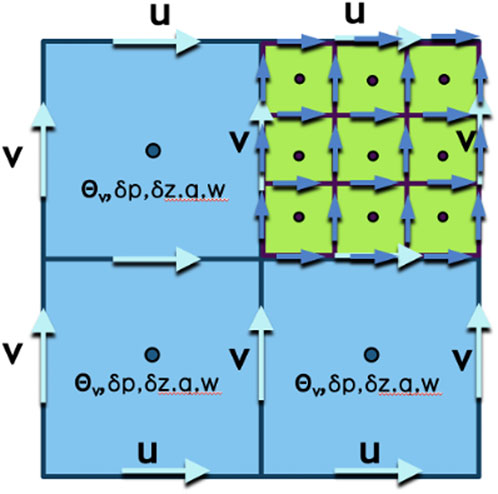
Figure 1. Diagram of placement of prognostic variables as cell average mass values, and staggered edge values for wind. Variables are eastward wind (u). Northward wind (v), virtual potential temperature (Θ_v), vertical delta of pressure (δp), vertical delta of geometric height (δz), moisture species (q), vertical velocity (w).

3.2 Nesting

Harris and Lin, 2013 introduced static nesting with high-resolution nests aligned to the parent grid (Figure 1). Horizontal alignment means that for 3X nest resolution, nine high-resolution grid cells will fit exactly in a single parent grid cell. This alignment permits exact conservation of quantities when summed from the high-resolution cells in the nest, and improved computational efficiency. While vertical nesting is also provided by the static-nest functionality, it is beyond the scope of this moving nest implementation.

The static nest functionality of the UFS permits multiple nests as well as telescoping nests (Mouallem et al., 2022). This initial implementation of HAFS detailed in this paper allows a single moving nest without telescoping. In later work, we plan to extend the moving nest functionality to multiple moving nests and telescoping nests.

The WRF model restricted nesting refinement ratios to odd numbers only; most often used were 3x and 5X. Even numbered refinement ratios were not permitted due to the grid staggering used in WRF. Due to the grid layouts of the FV3 dynamic core, odd and even refinement ratios are permitted by the static nesting code. On the global cubed sphere layout, the surface of the Earth is projected onto 6 square cube faces. Each nest currently must remain on a single parent cube face, without crossing onto another cube face (Mouallem et al., 2022). Later work may permit us to allow nests to cross cube edges and corners. In a regional configuration, the nest can be positioned on any portion of the regional parent grid. In each configuration, the nest edge must remain several points away from the parent cube face edge, due to requirements for neighboring points for differencing schemes in the model.

Nest motion in the UFS is accomplished by shifting the nest one coarse grid cell in the x and/or y direction at a time. When the nest is moved, the high-resolution points at the leading edge need to be filled in with a full set of consistent and balanced surface and atmospheric data. There are five different types of model variables that need to be shifted or recalculated when the nest is moved forward. The variable types are prognostic atmospheric variables, physics variables, surface fields, land-masked surface fields, and navigation fields. The method of generating the high-resolution data of each of these types will be described in this section.

Nest motion in the UFS is configured using namelist options; there are capabilities for prescribed motion in a constant direction and storm-following. Configuration options allow setting the number of model timesteps that should be executed before the next evaluation of whether the nest should be moved.

3.3 Nest motion steps

For prognostic and physics fields that evolve during the forecast run, the following nest motion algorithm that leverages the nest halo concept shown in Figure 2 from the original implementation of the FV3 dynamic core is used. The processor layout defined in the namelist files assigns a set of processors to the parent grid(s), and a separate set of processors to the nest grid. Each processor manages a rectangular grid of points in the x/y direction. For nest processors, the Flexible Modeling System (FMS) layer tracks how each point connects to the parent point and processor.

Figure 2

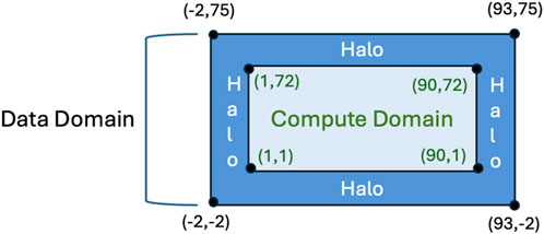
Figure 2. Schematic diagram of layout of data domain, compute domain, and halo for a single processor in the model. The compute domain in this example encompasses 90 points in the x-direction, numbered from 1–90, and 72 points in the y-direction numbered from 1–72. A halo region for communication with neighboring processors is made up of 3 points in the x- and y-directions surrounding the compute domain. The union of the halo region and compute domain is defined as the data domain, extending from −2 to 93 in the x-direction, and from −2 to 75 in the y-direction.

When the storm tracker code has determined the nest should be moved on this timesteps, the following steps are executed as shown in Figure 3:

0 –Figure 3A shows the starting state, before the nest move begins.

1 – Figure 3B shows the coarse data interpolated to leading edge of nest.

2 –Figure 3C shows that the leading edge has been populated.

3 – Figure 3D shows the halo data being shifted between processors (PEs) internal to nest.

4 – Figure 3E shows that all halos have been populated with variable data.

5 – Figure 3F shows the internal arrays shifted on each PE, with the nest move fully complete, and the model state ready for next dynamics timestep.

Figure 3

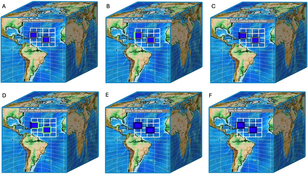
Figure 3. (A–F): Diagrams showing steps 0–5 of filling halos with data to accomplish a nest move, illustrating the handling of PEs on the leading edge of the nest, and internal to the nest. The white rectangles indicate the compute domains for each nest processor that make up the entire nest grid, in a 4x4 decomposition. Grey fill indicates data that needs to be updated before the nest move can be completed. Dark blue fill indicates data that has been updated with values after a nest move. Land areas are shaded with topography, and ocean areas are shaded with bathymetry.

3.3.1 Nest move begins

Each processor manages a rectangular area of the parent or child grid. The set of grid cells where model dynamics and physics are integrated is called the compute domain. In order to have a sufficient number of adjacent values to calculate derivatives, a halo of 3 points of data beyond the edge of the compute domain is defined, and filled with valid data that was computed on the adjacent processors. The larger area that consists of the compute domain plus the halos is called the data domain.

When the nest move begins, the halos for all nest processors contain old data from the prior timestep, and need to be refilled.

3.3.2 Coarse data interpolated to leading edge of nest

The first action of the nest move is to fill the halos at the leading edge of the moving nest. In the case illustrated in Figure 3B the nest is shifting west, so the westernmost halo points in the nest (highlighted in yellow) are populated by interpolating from the coarse grid parent points. This action is performed by the nest processors requesting a buffer of coarse data values from the overlapping parent processors, which the parent processors send via MPI to the nest processors. Then the nest processor performs the interpolation to the finer nest resolution cells.

3.3.3 Leading edge has been populated

At this point, the leading edge of the nest has been populated with the necessary data, so we show the leading edge in dark blue.

3.3.4 Halo data shifted between processors (PEs) internal to nest

The next step is to populate the interior halos on the nest processors with data from the neighboring nest processors. This step does not require any interpolation, as the data on the neighboring processors is also at the fine nest resolution.

3.3.5 All halos have been populated

At this stage, all of the halos in the nest have been populated with up-to-date data.

3.3.6 Internal arrays shifted on each PE using fortran intrinsic function EOSHIFT - Ready for next dynamics timestep

The final step of the nest move involves shifting the data in the interior of the nest. Here, we use the Fortran intrinsic function EOSHIFT, which efficiently shifts an array of data. The data in the interior of the nest is shifted from the original nest offset location to the new nest offset location to reflect the position after the nest move. This step does not require any communication between processors.

3.4 Prognostic atmospheric variables

The explicit prognostic fields in the model are shifted with each nest move. This set includes a number of variables that represent the finite element averages on an Arakawa A-grid (Arakawa and Lamb, 1977). Horizontal winds are expressed as u- and v-components, staggered on a D-grid. The A-grid variables are potential temperature, vertical motion (w), grid cell thickness in geometric height (delz), grid cell thickness in pressure (delp), and arrays for moisture species. The moisture species include water vapor, as well as various forms of cloud water and cloud ice, plus precipitation species. These variables could also include items such as cloud fraction. The water species will vary depending on the microphysics scheme chosen.

These fields are moved using the method detailed in steps 0–5 above.

3.5 Physics variables

Physics variables which vary during the model run such as surface roughness, surface temperature, soil temperature, soil moisture, vegetation canopy moisture, and lake parameters, among others, that are parts of the model physics or NOAA’s Common Community Physics Package (CCPP) (Heinzeller et al., 2023) are also shifted with each nest move. For computational efficiency, the physics variables are stored and calculated in 1-D arrays or blocks, to enable efficient vectorization by the Fortran compiler.

Each time the nest moves, the 1-D arrays of physics data for each variable on each nest PE are copied into temporary 2-D arrays in the same shape as the atmospheric prognostic variables. These temporary variables are then shifted using the same subroutines as for the prognostic variables, with values interpolated from the coarse parent grid at the nest leading edge, values communicated to neighboring nest PEs along the internal boundaries, and the remainder of values shifted on each PE using the Fortran intrinsic function EOSHIFT. After the shifting step has been completed, the values in the updated 2-D arrays are copied into the 1-D vectors for the rest of the model to use at the next timestep.

3.6 High-resolution static surface fields

Many surface fields, such as terrain, land/sea/ice mask, vegetation type, and more, remain static during a weather-scale (0–10 days) forecast run. These are transferred onto the forecast grid during preprocessing. To gain the maximum benefit of the increased resolution in the moving nest, we use these fields at the high resolution of the nest. Additional fields are static inputs to quantities that are derived from surface properties and conditions that evolve with precipitation or other weather during the course of the forecast; these include albedo input variables for shortwave and longwave radiation which are combined with snow cover, solar zenith angle and potentially other quantities to produce the effective albedo at each forecast time.

3.7 Land-masked surface fields

A number of surface fields that vary during the course of a model run are also moved. These include emissivity, albedo, and surface roughness. These fields are also partitioned into different variables for land points, water points, and ice points. Interpolation of values is performed at the leading edge of the moving nest taking into account the land/sea/ice mask to only consider values from the same surface type. If no matching landmask values are found in the 3x3 square around the nest point, a default value is assigned instead using the same algorithm as model initialization.

3.8 Navigation fields

Another set of fields in the dynamic core are used for describing the location of the grid cells and corners in latitude/longitude coordinates, as well as cell edge distances, cell areas, the Coriolis terms for the point based on its latitude, and related terms. All of these fields are directly computable from the latitude/longitude coordinates of the supergrid components. For accuracy, these are computed in 64-bit precision in most configurations of the model. When the nest has been shifted, and the new latitude/longitude coordinates have been set for the leading edge of the nest, then these navigation fields are computed for the nest.

3.9 Terrain smoothing

The static nest code described in Harris and Lin, 2013, applies a smoothing algorithm to the terrain heights on the interior edge of the nest. The smoother blends the coarse-resolution terrain with the high-resolution terrain with linearly increasing weight to the high-resolution data over five points. The goal of this terrain smoothing is to reduce instabilities along the nest edge when it lies over areas of sharp terrain. Initial development of the moving nest did not implement this smoothing after nest moves, which led to the production of strong gravity waves when the moving nest encountered higher terrain, and occasional model crashes. We then introduced the same terrain smoothing algorithm along the nest interior edges after each nest move, greatly reducing gravity wave production and eliminating the model crashes.

3.10 Concurrent nesting

The moving nest algorithm uses the concurrent nesting strategy introduced in Harris and Lin 2013, which aids in the efficiency and accuracy of the model. The time-extrapolated boundary conditions at the nest edge computed during the previous time step are used by the nest time step calculations at the same time that the parent domain is performing its time step calculations. This allows the nest grids and parent grids to advance their time step in parallel on separate processors; a significant upgrade from nest behavior in WRF which time stepped the nests after the parent.

3.11 Automated storm tracker

In order for the nest to follow the center of a TC, we ported a version of the internal storm tracking code from HWRF to HAFS. This code is based on the GFDL vortex tracker (Marchok, 2021) with modifications to use prognostic and diagnostic fields available inside the model code and to skip the geographical smoothing from the original algorithm that would require expensive communication between nest PEs. The nest can move a single coarse grid cell in both the x- and y-direction at the same time, but it is not permitted to move 2 or more coarse grid cells in one direction at once.

The current implementation restricts the motion in the x- and y-directions to −1, 0, or +1 parent grid cells. This restriction is based on the use of the halo data structures and subroutines, which extend 3 grid cells beyond the edge of the computational domain. The restriction is also in place to enhance the stability of the model, by not interpolating a large number of cells at a single timestep. We have concerns that shifting multiple cells at once could lead to oscillations or other instabilities, and testing this has been beyond the current scope of our development. The variables used to track the storm are sea level pressure. At each level of 10 m above the surface, 850 mb, and 700 mb, vorticity, wind speed, and geopotential height are used. The center is calculated by averaging the centers from each of the variables, within 225 km of the previous center location. If no center can be determined, or the center is found beyond 225 km from the previous center location, nest motion is not performed for this timestep.

In the namelist for the forecast job, several options for the vortex_tracker are available. Option 1 allows hard-coded nest motion, which is useful for test cases, debugging, and research runs for weak systems without a discernible center. Option 2 will allow an intermediate nest to follow the highest resolution nest, when telescoped moving nests are implemented in a later upgrade. Option 3 is a simple tracking algorithm that only follows the minimum sea level pressure. This option may not follow the storm center properly if the nest encounters areas of terrain. Option 6 is adopted from the HWRF tracker, using a subset of the tracking variables. Option 7 is the most complete storm tracking algorithm, also based on the HWRF vortex tracker.

3.12 Feedback to parent grid

The nested grid performs two-way feedback to the parent grid at 100% using the same methods as the static nesting in UFS (Harris and Lin, 2013). Cell-centered variables are updated with the average of the nest cells that make up the parent cell. Wind values which are staggered on the D-grid are computed from cell faces. This method updates temperature, u-winds, v-winds but does not update dp. The lack of update of dp means that mass is conserved. This mass-conserving remapping update is demonstrated in Harris and Lin, 2013 to introduce only small errors or artifacts for a variety of meteorological conditions. For the hurricane model, the feedback allows the improvements in track and intensity of the storm due to resolution to propagate back to the larger environment.

3.13 Preprocessing

As part of the setup to run a model forecast, preprocessing steps are run to transform static datasets such as terrain, vegetation type, albedo, etc. From standardized input datasets onto the model grid. Some of these fields are purely static on a weather timeframe, such as terrain height. Other variables are interpolated to a daily value from monthly averages, for fields such as vegetation greenness, to account for seasonality.

For a static nest configuration, these fields are generated at the parent resolution for the parent grid, and at the high resolution for the nest. For moving nest configurations, we run an extra step in the preprocessing to generate all of these static fields prior to the model run at the high resolution but covering the area of the whole parent grid–either the full regional domain, or the parent cube face from the global cubed sphere. This allows the model to benefit from high-resolution surface data for the moving nest, rather than downscaling from the coarse parent grid at runtime. This means that the surface fields will have the same high resolution in the moving nest as they have at static nest initialization. This is particularly important when the hurricane within the nest makes landfall or encounters islands, so that full resolution of the land sea mask and terrain and associated properties can be utilized by the model. For current resolutions, this data can be handled by one file for each variable, covering the entire parent domain. As the parent grid size is expanded or resolution is increased, we will likely need to implement a tiling scheme for generating and reading these variables.

The current implementation of the model reads high-resolution grids into memory at startup, then repopulates the surface variables in the moving nest by copying the relevant section from the large high-resolution grid.

3.14 Performance

The code to perform the nest moves makes calls to many of the subroutines and data structures defined in GFDL’s Flexible Modeling System (FMS) (Balaji, 2004). Important features provided by FMS include data structures to define the splitting of the parent and nest grids between all of the assigned processors (processor decomposition), and subroutines to arrange communication between a nest processor and the parent processors that overlap it. These communication subroutines ensure maximal parallelization and performance by requesting data from the exact parent processors to be sent to the nest processor, avoiding any aggregation of data which would slow performance and require synchronization between different processors.

Since the goal of nesting and moving nests is to be able to run forecasts that are highly efficient in CPU usage, we spent significant effort in performance profiling to find slow code segments and optimization efforts. Important considerations for fast performance include parallelization to allow each processor to run independently and reducing waiting on results from other processors as much as possible. The moving nest code was designed to follow the parallelization strategy used by the existing static nest code. This means that the bulk of the computation to accomplish a nest move occurs on the processors allocated to the nest grid cells.

The initial architecture of the moving nest algorithm relies on the existing halo subroutines in the FMS subsystem. (Balaji, 2004). The halo subroutines allow the nest PE to communicate with only the necessary parent PEs to gather the needed data, allowing efficient and highly parallel operations. Away from the nest edges, all of the nest variables need to be shifted to their new coordinates when nest motion occurs. This operation occurs on each nest PE independently. Parent PEs do no processing during this step. We leveraged the Fortran intrinsic function EOSHIFT, which performs the shift of array elements. Since this is a built-in function, its performance is very fast.

Performance profiling revealed some bottlenecks in the nest motion algorithm, so these were rewritten to speed the code. After these optimizations, testing compared moving nest cases with identically-sized static nest configurations, and found the moving nest code added between 3% and 7% to the wallclock runtime.

4 Results and discussion

Below, we will discuss forecast results and performance for several configurations of the model for Hurricane Ian (2022), both in global and regional configurations. More detailed analysis of the 2022 North Atlantic season with a regional configuration of the model is provided in Hazelton et al., 2023. For the North Atlantic 2022 season, two HAFS configurations with moving nest showed track skill improvements compared to the operational HWRF from forecast hours 24–60, and slight improvements to neutral from hours 60–108.

4.1 Global model configuration

The moving nest is implemented in the regional as well as the global cubed sphere configurations of UFS. We believe this is the first moving nest ever implemented for a global NWP model. A global configuration offers a number of benefits in terms of scientific improvements and operational efficiency. Consistency of the model dynamics and physics for the globe is achieved by removing a dependency on lateral boundary conditions, which are generally from a model with different resolutions, and potentially different dynamical cores and physics parameterizations. The lateral boundaries are often the site of artifacts in many atmospheric fields. Enabling the global moving nest model to start with only initialization files, either from another model or from a data assimilation system, can allow an operational forecast system to begin earlier, leading to more timely forecasts.

The global moving nest configuration consists of 6 tiles to cover the globe in the cube sphere configuration, and the moving nest at with nest refinement factor of 3 on tile 6. A schematic diagram of the moving nest on a global cubed sphere is shown in Figure 4. The global resolution of C768 which corresponds to grid cells with spacing of approximately 13 km in the horizontal; the nest refinement of 3X yields nest resolution at approximately 4 km. For the run shown below, tile 6 and the moving nest are centered on the initial storm location based on the NHC advisory.

Figure 4

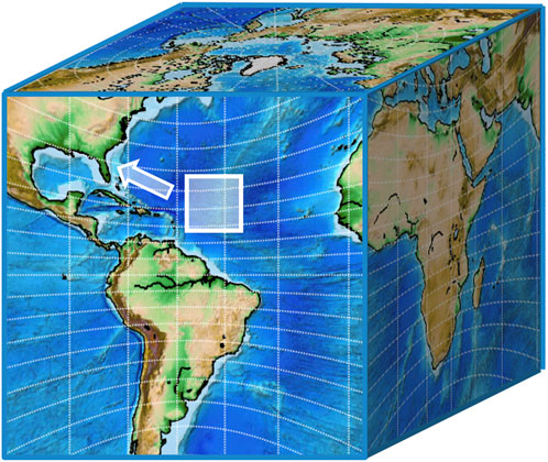
Figure 4. Schematic of moving nest on a global cubed sphere configuration.

The global grids remain static throughout the model run. The global grid was configured with tile 6 centered at 23.5N and 83.3W, based on the advisory location of the storm at model initialization time (National Hurricane Center, 2022). The moving nest grid at 4 km resolution spans 720 X 720 grid cells, or approximately 25^o X 25^o of latitude and longitude, and is initialized at the center of the tile 6 grid. The nest was allowed to move every 2 timesteps, following the storm center based on the storm tracking algorithm. The nest can move one coarse grid cell in the x and y directions at a time. A storm moving slower than 160 km/h will be accurately followed by these settings. If the nest reaches the edge of the parent cube face, nest motion is stopped.

The model is run with 81 vertical levels on a terrain-following sigma coordinate in both the parent and nest. Physics options chosen are GFDL microphysics and the NOAH land surface model. New model variables that are introduced by a physics parameterization must be explicitly handled in the moving nest code, so at present, not all of the CCPP physics parameterizations are currently supported in the moving nest code.

For simplicity, we use a cold start initialization directly from the GFS global analysis. While the real-time parallel experiment (Hazelton et al., 2020) and operational implementation use vortex initialization and data assimilation to improve the analysis of the TC at initialization, we omit those steps here to focus solely on the functionality of the moving nest. Boundary conditions are not required for a global run; instead, initial conditions are generated for all grid cells on the globe, and then the forecast can be time-stepped forward.

The model timestep dt_atmos is 90s. For the nest we use a vertical remapping factor of five and an acoustic timestep factor of 9. These options mean that the physics are called every 90s, vertical remapping is called every 18s, and dynamics are called every 2s. The global parent uses a vertical remapping factor of 2 and an acoustic timestep factor of 5, so that for the nest, physics are called every 90s, vertical remapping is called every 45s, and dynamics are called every 9s.

The parent grid is coupled to the HYCOM ocean model, with two-way flux feedback coupling frequency every 4 timesteps, or every 6 min. The ocean model domain covers the North Atlantic and East Pacific basins from 23°S to 46°N and 178°W to 15°E. Sea surface temperature updates from the ocean model are downscaled to the moving nest when it moves and on every coupling timestep.

Each of the 6 global tiles is distributed onto 12x10 processors, for a total of 720 processors. The nest is also distributed onto 12x10 processors, and 120 processors are allotted for parallel writing of forecast result files (the write_grid component). The total number allotment for this run is 960 processors, and the forecast completed in 26,428 s, or just over 7 h.

4.2 Example case forecast results

Hurricane Ian began as a tropical wave moving off of Africa, and intensified to a tropical depression in the southern Caribbean on 23 September 2022 at 13.9°N 69.6°W. It reached hurricane intensity on 26 September 2022 at 09Z SW of the Cayman Islands in the Caribbean Sea. The hurricane then crossed western Cuba, emerging into the SE Gulf of Mexico on 27 September. After quickly reorganizing, the storm intensified and underwent an eyewall replacement cycle, and made landfall near Cayo Costa, FL around 1905Z on 28 September 2022 with a maximum sustained windspeed of 130 kts and central pressure of 940 mb (Bucci et al., 2023).

The global forecast for Ian was initiated at 18Z on 27 September 2022 when Ian had just emerged into the Gulf of Mexico after crossing western Cuba at 23.5°N 83.3°W. The NHC advisory at that time indicated maximum sustained winds of 120 mph and a minimum central pressure of 955 mb.

Figure 5 shows the initial location of the nest on the global tile. The nest moved 664 times during the 126 h forecast run, around 5 times per hour.

Figure 5

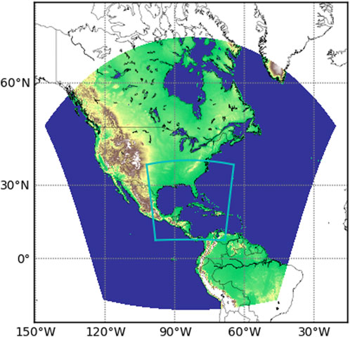
Figure 5. Configuration of global tile 6 and initial position for moving nest for Hurricane Ian forecast initialized on 20220927 18Z.

The evolution of the storm is shown in Figure 6, as Ian moves from near Cuba at forecast hour 0 to landfall in SW Florida at hour 24 then up the Florida peninsula at forecast hours 36 and 48. The storm and moving nest are shown moving through the Gulf of Mexico, making landfall in Florida, and emerging east of Florida. This demonstrates the ability of the moving nest code to handle moving the atmospheric variables, as well as the various surface physics and terrain fields. It also shows that the automated storm tracker follows the storm center over the open ocean as well as across land masses.

Figure 6

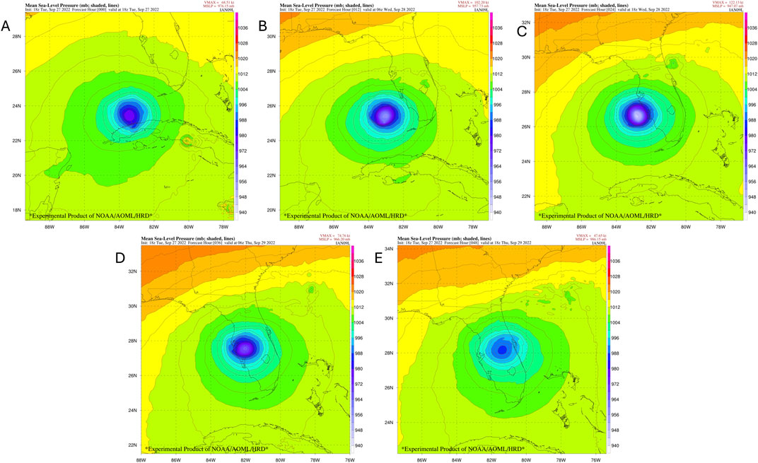
Figure 6. Timeseries of mean sea level pressure (MSLP) in millibars forecast hours 0 to 48 of moving nest for global simulation of Hurricane Ian, initialized 20220927 18Z.

The azimuthal mean tangential wind for the global run is shown in the time series in Figure 7, from hour 0 to hour 48. The storm reaches maximum intensity of 948 hPa central pressure and 107 kts maximum winds in the 24 h forecast, which was about 1 h before landfall. With the cold start from the coarser-resolution global GFS, the initial radius of maximum winds is near 60 km. The 12 and 24 h forecasts best show the structure of the eyewall, with a radius of maximum winds decreasing to about 40 km by the 24 h forecast. After landfall, in the 36 and 48 h forecasts, we see the wind speeds decreasing and the radius of maximum winds spreading as the storm weakens.

Figure 7

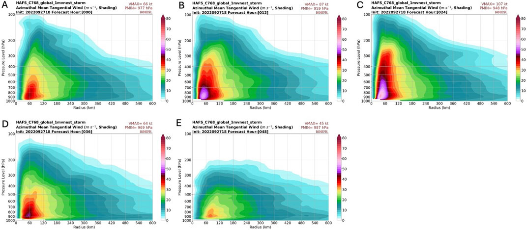
Figure 7. (A–E) shows the azimuthal mean of tangential wind of the inner nest of the global run, from forecast hour 0 to forecast hour 48.

4.3 Regional model configuration

A regional model configuration that was tested for operational implementation was used for these runs. In this configuration, a parent grid at 6 km resolution and a moving nest at 2 km resolution are run for a 126 h forecast. A parent grid at 6 km resolution spanning 1,320 X 1,320 grid cells, or approximately 90^o X 90^o of latitude and longitude, is centered on the initial storm location based on the NHC Best Track dataset, as shown in Figure 8. This grid remains static throughout the model run. The moving nest grid at 2 km resolution spans 600 X 600 grid cells, or approximately 15^o X 15^o of latitude and longitude, and is initialized at the center of the parent grid. The model timestep dt_atmos is 90s.

Figure 8

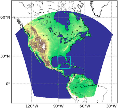
Figure 8. Moving nest initial location on terrain of parent regional grid for Hurricane Ian 20220927 18Z case.

The parent regional nest has a remapping factor set at 2 and an acoustic timestep factor set at 5. These options mean that the physics are called every 90s, vertical remapping is called every 45s, and dynamics are called every 9s. The moving nest has a remapping factor set at 4 and an acoustic timestep factor set at 9. These options mean that the physics are called every 90s, vertical remapping is called every 15s, and dynamics are called every 2.5s. The nest will be allowed to move every 2 timesteps, following the storm center based on the storm tracking algorithm.

The model is run with 81 vertical levels on a terrain-following sigma coordinate in both the parent and nest. Physics options chosen are GFDL microphysics and NOAH land surface model. New model variables that are introduced by a physics parameterization must be explicitly handled in the moving nest code, so at present, not all of the UFS physics parameterizations are supported in the moving nest code.

As with the global case, we use a cold start initialization directly from the GFS global analysis. Vortex initialization and data assimilation are omitted. Boundary conditions at the edge of the parent regional grid are supplied every 3 h from the GFS global forecast.

The parent grid is coupled to the HYCOM ocean model, with two-way flux feedback coupling frequency every 4 timesteps, or every 6 min. Sea surface temperature updates from the ocean model are downscaled to the moving nest when it moves and on every coupling timestep.

The parent grid runs on 600 processors, in a 30x20 decomposition. The nest grid runs on an additional 600 processors, also in a 30x20 decomposition. Total wallclock runtime was 14,913 s, or just over 4 h.

4.4 Forecast results

For consistency, the regional forecast for Ian was initiated at the same time as the global case, 18Z on 27 September 2022, when Ian had just emerged into the Gulf of Mexico after crossing western Cuba. In order to concentrate demonstrating the moving nest features, we initialized with a cold start directly from the GFS; no extra data assimilation, vortex relocation, or vortex initialization was performed. The operational implementation uses more elaborate vortex-scale initialization for improved storm intensity, structure, and location for the model initial conditions.

The nest moved 1,387 times during the 126 h forecast run, around 10 times per hour. Figure 9 shows the track of this model run compared with the best track and other operational models. The storm and moving nest are shown moving through the Gulf of Mexico, making landfall in Florida, and emerging east of Florida. The track from HAFS aligns very well with the best track in the Gulf of Mexico and crossing Florida, then has a left bias as the storm moves northward into the Southeast.

Figure 9

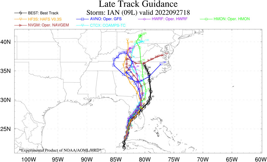
Figure 9. Hurricane Ian Track from HAFS model run in orange, compared with other operational models and best track.

Figure 10 shows the mean sea level pressure on the static parent grid at 12 hourly intervals from the forecast initialization through hour 48.

Figure 10

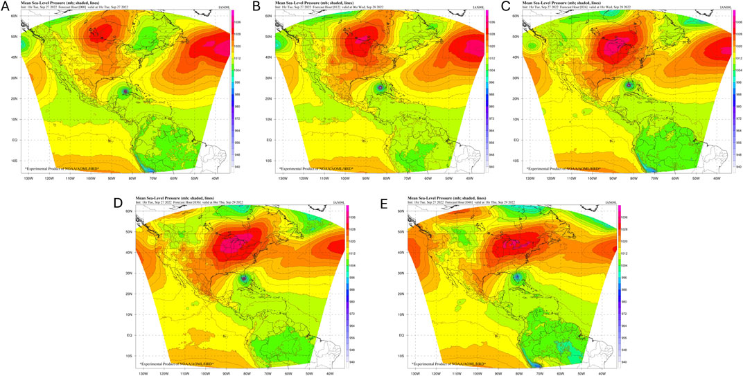
Figure 10. Plots of Parent Domain Mean Sea Level Pressure forecast hour 0, 12, 24, 36, 48.

The time series of parent (Figure 10) and nest (Figure 11) plots of mean sea level pressure shows the storm evolution in the regional configuration from forecast hour 0 to forecast hour 48, as Ian intensifies up in the Gulf of Mexico until making landfall in SW Florida, then crossing the peninsula.

Figure 11

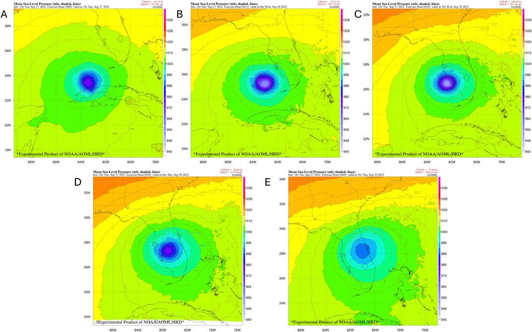
Figure 11. Plots of Nest Mean Sea Level Pressure forecast hours 0, 12, 24, 36, 48.

This demonstrates the ability of the moving nest code to handle moving the atmospheric variables, as well as the various surface physics and terrain fields. It also shows that the automated storm tracker follows the storm center over the open ocean as well as across land masses.

The azimuthal mean tangential wind for the regional run is shown in the time series in Figure 12, from hour 0 to hour 48. The storm reaches maximum intensity of 952 hPa central pressure and 109 kts maximum winds in the 24 h forecast, which was about 1 h before landfall. These values are similar to the 948 hPa and 107 kts seen in the global run. With the cold start from the coarser-resolution global GFS, the initial radius of maximum winds is near 60 km. The 12 and 24 h forecasts best show the structure of the eyewall, with a radius of maximum winds decreasing to about 40 km by the 24 h forecast. After landfall, in the 36 and 48 h forecasts, we see the wind speeds decreasing and the radius of maximum winds spreading as the storm weakens.

Figure 12

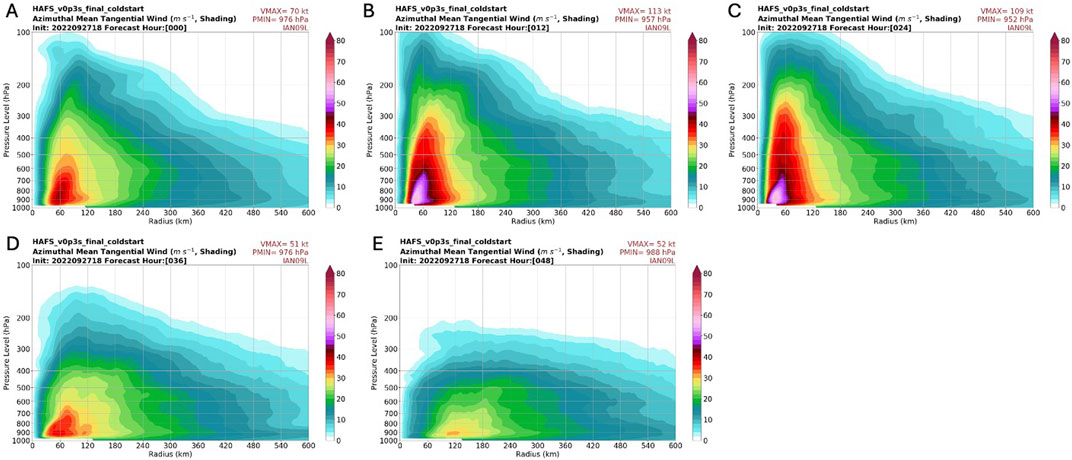
Figure 12. (A–E): Plots of the azimuthal mean of tangential wind of the inner nest of the global run, from forecast hours 0,12, 24, 36, 48.

4.5 Comparison with flight level data

The maintenance and development of the warm-core structure and inner-core winds are central to the intensification of hurricanes. For the first time, we have used flight-level observations to evaluate the structure and development of the temperature, humidity, and wind structure of the hurricane in the HAFS high-resolution moving nest. This will allow us to verify that the combination of model dynamics and physical parameterizations are capturing the structure of the storm.

In this section we verify the performance of the high-resolution nest in depicting the inner core structure of hurricanes by comparing the key prognostic variables in the model against the flight level data. The software was created to mine data from the model along the flight tracks. We have performed several forecast runs for Hurricane Ian (2022) to compare with flight level data from the NOAA P3 observations of wind velocity, temperature, and dewpoint. These retrospective regional runs were performed to match times when the reconnaissance aircraft was sampling the storm; the in-flight measurements are generally taken near the 700 mb level. Model runs were executed on storm-centered domains, with a 2 km resolution moving nest and a 6 km parent. Many other sources of in situ observations are also available such as radar and Stepped Frequency Microwave Radiometer (SFMR) data, which could be used to further validate the accuracy of the forecasts in future work.

4.5.1 Hurricane Ian 20220926 00Z model initialization

The first forecast run we compare with in-flight observations is from 20220926 00Z when Ian was in the Western Caribbean to the SW of Cuba and had just been upgraded to hurricane intensity of 65 knots. Analytics were run to center the modeled storm with the observed center location then compare flight-level winds, temperature, dewpoint with the modeled values. Figure 13A shows the flight track, while Figures 13B–D compare wind speed, temperature, and dewpoint values. We see excellent agreement between the observed values shown with the blue lines vs the modeled values shown with the brown lines. The wind plots show the most fine-scaled details, which match quite well between observations and model; with an accurate portrayal of the winds in the sectors of the storm that were sampled.

Figure 13

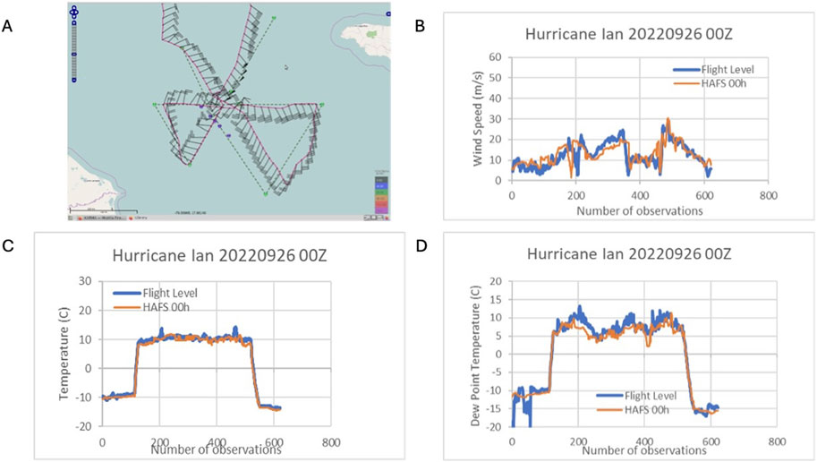
Figure 13. Hurricane Ian Model Initialization from 20220926 00Z compared with flight-level observations. (A). Shows the flight track (image courtesy of: NOAA) (B). Comparison of observations vs model wind speed in m/s (C). Comparison of observations vs model temperature. (D). Comparison of observations vs model dew point.

In Figure 13B, we compare wind speeds at flight level from the reconnaissance aircraft with the modeled values. The flight legs begin in the NW, with relatively light winds for a long flight segment. Around observation 200, we see that both the observations and model wind speeds have peaks around 20 m/s on either side of a nearly calm eye. From observations 220–350, we see windspeeds slowly increasing from around 15 m/s to around 25 m/s as the aircraft heads SE, then NE, then W in the SE sector of the storm. From observations 350–460, lighter windspeeds are observed and modeled in the SW sector of the storm. Just after observation 460, the flight track passes through the most intense part of the storm, just to the NE of the center, with observed and modeled windspeeds approaching 30 m/s, in line with the advisory intensity of 65 kts. Windspeeds then decrease rapidly as the flight track continues to the NE away from the storm center.

The comparison between observed and modeled windspeeds demonstrates that the model has accurately modeled the storm structure and asymmetries. In particular, the model accurately captured the relatively weak winds in all quadrants of the storm except for the NE.

In Figure 13C, we compare air temperature at flight level between the aircraft observations and the model. The temperature plot shows nearly constant values of approximately 10°C from around observation 150 to observation 550. The observations show two small temperature peaks around observation 200 and 460 as the flight neared the center of the storm; these do not seem to be captured by the model.

More interesting is the dewpoint data in Figure 13D. The flight legs spanning observations 150 to observation 550 correspond to the nearly constant temperature of 10°C. The dewpoint depression demonstrates dry air between observations 201–360 (in the SW quadrant of the storm), with the model broadly in agreement with the observations, but with the model a bit drier in the section from around observation 200–230.

This case shows that the HAFS model captured the structure and asymmetries of the storm as it was reaching hurricane intensity. The strongest windspeeds are accurately modeled to the NE of the storm center, and dry air was accurately modeled to the SW of the center.

4.5.2 Hurricane Ian Model Initialization 20220926 12Z

A subsequent model run was initialized at 20220926 12Z when Ian had intensified to a 100 kt hurricane and was passing over western Cuba. Flight observations were taken a few hours later as the storm had moved into the Gulf of Mexico. After adjustments for the offset of storm center location, the observations shown in Figure 14 also are in quite close agreement with the modeled values for wind speed, temperature, and dewpoint. We notice warming of the inner core, larger area of dew points above 10°C, and intensification of winds. When examining the plot of wind speed, we see a general agreement of the maximum intensity around 35 m/s, though the exact placement of some of the peak winds is offset radially a few kilometers.

Figure 14

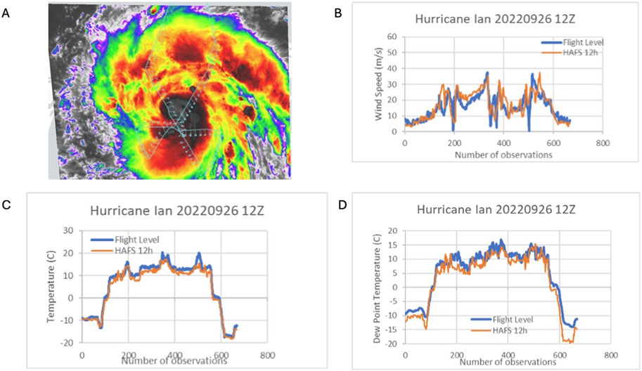
Figure 14. Hurricane Ian Model Initialization from 20220926 12Z compared with flight-level observations. (A). Shows the flight track (image courtesy of: NASA MTS) (B). Comparison of observations vs model wind speed in m/s (C). Comparison of observations vs model temperature. (D). Comparison of observations vs model dew point.

Figure 14B shows a comparison of flight-level observations with modeled windspeeds. The first flight leg is an approach from the N and NW of the storm center, shown in observations 0–200. Around observation 200, the flight crosses the center of the storm, with observed winds near 0; the modeled winds drop to approximately 6 m/s in the same area. The flight then samples the SE quadrant of the storm from observation 200–360. Windspeeds are stronger in this entire section of the storm, with maximum values just under 40 m/s observed to the immediate E of the center. From about observation 400–480, the aircraft samples the weaker SW quadrant of the storm, with observed windspeeds generally below 20 m/s. The model shows a similar trend but with some short sections of stronger winds. From observations 480–550, the aircraft passes from SW to NE through the center of the storm, again observing windspeeds just below 40 m/s. The aircraft observes windspeeds near 0, indicating it has located the storm center. The model values remain above 15 m/s in this segment, indicating that the storm center in the model is not completely aligned with the observed location. After observation 550, the windspeeds decrease as the aircraft continues to the NE away from the storm center.

Figure 14C shows the comparison between observed and modeled flight-level temperatures. Observed and modeled temperatures range from 10°C to 15°C from observations 150–550 when the aircraft is taking low-level samples. Three peaks in observed temperature are observed near observations 200, 360, and 500, corresponding to the times when the aircraft near or through the storm center. The model values are in general agreement with the observed temperatures, but at each peak, the model values are slightly lower than the observed maximum temperature.

Figure 14D shows the comparison between observed and modeled flight-level dewpoints. It is notable that the flight-level observations at center crossings near observations 200, 360, and 500 each show dewpoints lower than the temperature peaks at those locations, indicating passage through the somewhat dry eye, despite it containing some clouds as shown in 14a due to land interaction with western Cuba. Dewpoints from the model generally follow the trend of the observations, but with values a few degrees C lower especially in the NW quadrant in observations 100–200. For later observations, the general trend is for agreement between the observations and modeled values, but the fine-scale variations do not align. This is expected behavior as variations due to individual convective elements are not likely to be accurately represented.

Overall, comparison of flight-level observations with model values from this case shows that the model accurately captures many features of the storm, including the maximum intensity of the storm (as measured by windspeed) and the lack of a fully dry eye.

5 Summary

A moving nest algorithm for the FV3 dynamic core of the HAFS system has been implemented for global and regional configurations, and it provides stable and accurate model forecasts following the TC along its path. Preprocessing infrastructure generates static fields to exploit the full resolution of terrain and landcover datasets. During model execution data is needed at the leading edge of the nest when it moves. Prognostic fields and physics variables are interpolated from the coarse parent grid. Surface parameters are read from high-resolution files, and navigation values such as grid cell areas and length of cell edges are calculated from latitude and longitude points.

The moving nest code performs efficiently, adding between 3% and 7% runtime overhead compared to a static nest of the same dimensions. This allows researchers and operational centers to benefit from storm-scale nests that run significantly faster than a configuration with a static nest large enough to encompass a multi-day storm track. Analysis of global and regional cases shows accurate modeling of the intensity and track of a landfalling hurricane. Comparison with flight-level observational data confirms that the model reproduces many features of the storm structure and intensity distribution. Further studies will analyze the performance of the model over entire tropical cyclone seasons.

Data availability statement

The raw data supporting the conclusions of this article will be made available by the authors, without undue reservation.

Author contributions

WR: Conceptualization, Data curation, Investigation, Methodology, Software, Validation, Visualization, Writing–original draft, Writing–review and editing. XZ: Conceptualization, Funding acquisition, Methodology, Project administration, Resources, Supervision, Writing–review and editing. KA: Data curation, Investigation, Software, Validation, Writing–review and editing. SG: Conceptualization, Funding acquisition, Investigation, Methodology, Project administration, Resources, Software, Supervision, Visualization, Writing–review and editing.

Funding

The author(s) declare that financial support was received for the research, authorship, and/or publication of this article. This work was funded in part by: NOAA Award NA19OAR0220186, titled “Accelerate development of operational capability for multiple high resolutions moving nest.” NOAA FY18 Hurricane Supplemental IFAA 1A.4a, 3A.1, 3A.2 NOAA/NWS/OSTI UFS R2O Hurricane subproject NOAA Hurricane Forecast Improvement Project.

Acknowledgments

We would like to acknowledge the work of Bin Liu from NOAA EMC/Lynker on the model workflow software. Lucas Harris, Joseph Mouallem, Rusty Benson, and Zhi Liang from NOAA/GFDL provided very helpful guidance on the use of FMS and details about the FV3 dynamic core. Bin Liu and Chunxi Zhang [NOAA/EMC, current affiliation Climavision] provided significant expertise on identifying the necessary physics to be moved during nest motion steps. We would also like to acknowledge Ghassan Alaka [NOAA/AOML], Andrew Hazelton [U. Miami CIMAS, NOAA/AOML], and Russell St. Fleur [U. Miami CIMAS, NOAA/AOML] for the graphics suite that generates the track and sea level pressure plots. Figure 14a is from NASA’s Mission Tools Suite (MTS). The Mission Tools Suite (MTS) is the unified endpoint for many of the key enabling technologies available through the NASA Airborne Science Program’s sensor network. MTS is used for observing real-time telemetry from remote sensing platforms in concert with meteorological, airspace, satellite, and other mission products. A primary objective of MTS is to improve situational awareness for mission participants and to increase the efficiency and effectiveness of flight missions.

Conflict of interest

The authors declare that the research was conducted in the absence of any commercial or financial relationships that could be construed as a potential conflict of interest.

Publisher’s note

All claims expressed in this article are solely those of the authors and do not necessarily represent those of their affiliated organizations, or those of the publisher, the editors and the reviewers. Any product that may be evaluated in this article, or claim that may be made by its manufacturer, is not guaranteed or endorsed by the publisher.

References

Alaka, G., Sippel, J., Zhang, Z., Kim, H., Marks, F., Tallapragada, V., et al. (2024). Lifetime performance of the operational hurricane weather research and forecasting (HWRF) model for North Atlantic tropical cyclones. be Publ. Bull. Am. Meteorological Soc. Available at: https://journals.ametsoc.org/view/journals/bams/aop/BAMS-D-23-0139.1/BAMS-D-23-0139.1.xml (Accessed March 29, 2024). doi:10.1175/BAMS-D-23-0139.1

CrossRef Full Text | Google Scholar

Alaka, G., Zhang, X., and Gopalakrishnan, S. (2022). High-definition hurricanes: improving forecasts with storm-following nests. Bull. Am. Meteorological Soc. 103 (3), E680–E703. doi:10.1175/bams-d-20-0134.1

CrossRef Full Text | Google Scholar

Balaji, V. (2004). FMS: the GFDL flexible modeling system. Available at: https://data1.gfdl.noaa.gov/summer-school/Lectures/July19/01_Balaji_fms-am3.pdf.

Google Scholar

Bender, M., Marchok, T., Tuleya, R., Ginis, I., Tallapragada, V., and Lord, S. (2019). Hurricane model development at GFDL: a collaborative success story from a historical perspective. Bull. Am. Meteorological Soc. 100 (9), 1725–1736. doi:10.1175/bams-d-18-0197.1

CrossRef Full Text | Google Scholar

Bucci, L., Alaka, L., Hagen, A., Delgado, S., and Beven, J. (2023). National hurricane center tropical cyclone report hurricane ian. (Al092022) 23-30 Sept., 2022. Available at: https://www.nhc.noaa.gov/data/tcr/AL092022_Ian.pdf.

Google Scholar

Doyle, J. D., Hodur, R., Chen, S., Jin, Y., Moskaitis, J., Wang, S., et al. (2014). Tropical cyclone prediction using COAMPS-TC. Oceanography 27, 104–115. doi:10.5670/oceanog.2014.72

CrossRef Full Text | Google Scholar

Gopalakrishnan, S., Marks, F., Zhang, X., Bao, J., Yeh, K., and Atlas, R. (2011). The experimental HWRF system: a study on the influence of horizontal resolution on the structure and intensity changes in tropical cyclones using an idealized framework. Mon. Weather Rev. 139 (6), 1762–1784. doi:10.1175/2010mwr3535.1

CrossRef Full Text | Google Scholar

Gopalakrishnan, S. G., Surgi, N., Tuleya, R., and Janjic, Z. (2006) “NCEP’s two-way interactive-moving-nest NMM-WRF modeling system for hurricane forecasting,” in 27th conf. On hurricanes and tropical meteorology, 7A.3. Monterey, CA: Amer. Meteor. Soc. Available at: https://ams.confex.com/ams/pdfpapers/107899.pdf.

Google Scholar

Harris, L., and Lin, S.-J. (2013). A two-way nested global-regional dynamical core on the cubed-sphere grid. Mon. Wea. Rev. 141, 283–306. doi:10.1175/MWR-D-11-00201.1

CrossRef Full Text | Google Scholar

Harrison, E. (1973). Three-dimensional numerical simulations of tropical systems utilizing nested finite grids. J. Atmos. Sci. 30 (8), 1528–1543. doi:10.1175/1520-0469(1973)030<1528:tdnsot>2.0.co;2

CrossRef Full Text | Google Scholar

Hazelton, A., Alaka, G. J., Gramer, L., Ramstrom, W., Ditchek, S., Chen, X., et al. (2023). 2022 real-time Hurricane forecasts from an experimental version of the Hurricane analysis and forecast system (HAFSV0.3S). Front. Earth Sci. 11, 1264969. doi:10.3389/feart.2023.1264969

CrossRef Full Text | Google Scholar

Hazelton, A., Zhang, X., Gopalakrishnan, S., Ramstrom, W., Marks, F., and Zhang, J. A. (2020). High-resolution ensemble HFV3 forecasts of Hurricane Michael (2018): rapid intensification in shear. Mon. Wea. Rev. 148, 2009–2032. doi:10.1175/MWR-D-19-0275.1

CrossRef Full Text | Google Scholar

Heinzeller, D., Bernardet, L., Firl, G., Zhang, M., Sun, Xi., and Ek, M. (2023). The Common community physics package (CCPP) framework v6. Geosci. Model Dev. 16, 2235–2259. doi:10.5194/gmd-16-2235-2023

CrossRef Full Text | Google Scholar

Kerlin, J. (1979). Performance test of the movable-area fine-mesh model in the western pacific. National Meteorological Center (U.S.) office note 194. Available at: https://repository.library.noaa.gov/view/noaa/12174.

Google Scholar

Komaromi, W., Reinecke, P., Doyle, J., and Moskaitis, J. (2021). The naval research laboratory’s coupled Ocean–Atmosphere Mesoscale prediction system-tropical cyclone ensemble (COAMPS-TC ensemble). Weather Forecast. 36 (2), 499–517. doi:10.1175/waf-d-20-0038.1

CrossRef Full Text | Google Scholar

Kurihara, Y., and Bender, M. (1980). Use of a movable nested-mesh model for tracking a small vortex. Mon. Weather Rev. 108 (11), 1792–1809. doi:10.1175/1520-0493(1980)108<1792:uoamnm>2.0.co;2

CrossRef Full Text | Google Scholar

Kurihara, Y., Tripoli, G. J., and Bender, M. A. (1979). Design of a movable nested-mesh primitive equation model. Mon. Wea. Rev. 107, 239–249. doi:10.1175/1520-0493(1979)107<0239:DOAMNM>2.0.CO;2

CrossRef Full Text | Google Scholar

Kurihara, Y., Tuleya, R., and Bender, M. (1998). The GFDL hurricane prediction system and its performance in the 1995 hurricane season. Mon. Weather Rev. 126 (5), 1306–1322. doi:10.1175/1520-0493(1998)126<1306:tghpsa>2.0.co;2

CrossRef Full Text | Google Scholar

Marchok, T. (2021). Important factors in the tracking of tropical cyclones in operational models. J. Appl. Meteorology Climatol. 60 (9), 1265–1284. doi:10.1175/jamc-d-20-0175.1

CrossRef Full Text | Google Scholar

Mouallem, J., Harris, L., and Benson, R. (2022). Multiple same-level and telescoping nesting in GFDL's dynamical core. Geosci. Model Dev. 15, 4355–4371. doi:10.5194/gmd-15-4355-2022

CrossRef Full Text | Google Scholar

National Hurricane Center (2022). Tropical storm ian intermediate advisory number 9A. Available at: https://www.nhc.noaa.gov/archive/2022/al09/al092022.public_a.009.shtml? (Accessed March 13, 2024).

Google Scholar

Phillips, N. (1978). A test of finer resolution. Natl. Meteorol. Cent. (U.S.). Available at: https://www.ncep.noaa.gov/officenotes/NOAA-NPM-NCEPON-0002/013BA1E1.pdf.

Google Scholar

Shuman, F. (1989). History of numerical weather prediction at the national meteorological center. Weather Forecast. 4 (3), 286–296. doi:10.1175/1520-0434(1989)004<0286:honwpa>2.0.co;2

CrossRef Full Text | Google Scholar