Reverse time migration based on the body-fitted grid in pseudo-acoustic vertical transverse isotropic media with non-flat surface topography

As one of the main seismic imaging methods, conventional reverse time migration (RTM) may not produce high-quality images in areas with non-flat surfaces and anisotropy because the complex surfaces have a great impact on seismic wave simulation, resulting in strong scattering waves. In addition, in isotropic acoustic (ISO) RTM, the neglection of the anisotropic effects will lead to incorrect travel times during source and receiver wavefield extrapolation. To overcome these problems, we develop a topographic pseudo-acoustic vertical transverse isotropic (VTI) RTM algorithm based on the body-fitted grid. In this method, we first derive anisotropic pseudo-acoustic wave equations in the curvilinear coordinate system. Then, the Lebedev grid finite-difference scheme is used to update these equations to simulate wavefields. Finally, we use the source-normalized cross-correlation imaging condition to realize RTM. Numerical tests are performed to evaluate the feasibility and applicability of the proposed method. The imaging results show that the proposed method can remove the effect of surface topography and anisotropy on seismic wave propagation and improve migration imaging precision.

1 Introduction

The reverse time migration (RTM) algorithm (Baysal et al., 1983; McMechan, 1983), which is based on a two-way wave equation, has advantages in accurately imaging complex structures, compared to ray-based migration and one-way wave equation migration. It can deal with large lateral velocity variations and has no dip limitations on the images. Therefore, it has become an important seismic imaging method in the industry. However, non-flat surface topography introduces numerical problems for migration algorithms that are based on flat surface assumption (Reshef, 1991). Berryhill (1979) first used wave-equation datuming to reduce surface topography’s influence on migration results. Beasley and Lynn (1992) introduced the “zero-velocity layer” concept, which is an elegant technique for the error caused by the elevation-static correction. However, this technique cannot be applied to the computationally attractive phase-shift algorithms because it includes the non-physical characteristic of zero velocity (Bevc, 1997). Alternatively, without any datuming or elevation static corrections, some wave-equation-based methods that can directly simulate seismic wavefields and image seismic data recorded on an irregular topographic surface have been proposed. One method is to use smaller grid elements to approximate irregular surfaces (Robertsson, 1996; Ohminato and Chouet, 1997). However, staircase approximation leads to artificial scattering waves, which may affect the physical scattering waves or multiple reflection waves (Zhang and Chen, 2006). To avoid the artifacts caused by this staircase approximation, the other method employs vertical grid mapping to match the computational grid with surface topography (Tessmer et al., 1992; Hestholm and Ruud, 1994; Tarrass et al., 2011; Qu et al., 2017). It is effective for relatively smooth topography but has limitations for steep topography (Hayashi et al., 2001). In recent years, some researchers used the numerical simulation algorithm based on the body-fitted grid to tackle the undulating surface problem and obtained good results (Fornberg, 1988; Zhang and Chen, 2006; Appelö and Petersson, 2009). Then, the RTM based on this numerical simulation algorithm in the curvilinear coordinate was realized by Lan et al. (2014) and Qu and Li (2019). The body-fitted grid is conforming to the rugged surface, which can avoid artificial scattering waves. This is a coordinate transformation method, which maps the physical points with the curvilinear grid to the calculational points with the rectangular grid. In curvilinear coordinates, the partial differential wave equations are numerically updated by an optimized non-staggered finite-difference scheme, such as the DRP/opt MacCormack scheme (Zhang and Chen, 2006). Although the DRP/opt MacCormack scheme can essentially eliminate lattice oscillations, it needs a smaller grid length to achieve the same accuracy as the staggered grid scheme, which greatly increases the computational cost. To avoid wavefield interpolation using the standard-staggered grid (SSG) approach (Virieux, 1986), de la Puente et al. (2014), Konuk and Shragge (2021), and Sethi et al. (2022) used the Lebedev grid (LG, also known as the fully staggered grid) scheme (Lebedev, 1964) to accurately simulate wavefields on the curved grid.

Many rock-physics experiments and field measurements show that anisotropy is widely present in the subsurface media (Thomsen, 1986). The anisotropy mainly refers to velocity anisotropy, which will make seismic waves propagate at different speeds in different directions. If the anisotropic effect is ignored in seismic data processing, it will result in misplaced images and low resolution of the target during seismic migration and inversion. Although seismic anisotropy by nature is an elastic phenomenon, most anisotropic RTM implementations do not use the full elastic anisotropic wave equation because of the high computational cost involved (Chu et al., 2011). Then, many researchers derived simpler wave equations that can be solved efficiently to perform acoustic anisotropic RTM. Alkhalifah (1998) and Alkhalifah (2000) proposed the acoustic assumption approximation for transversely isotropic media with a vertical symmetry axis by setting the shear velocity along the axis of the symmetry to zero and developed a coupled pseudo-acoustic wave equation with the fourth-order partial derivatives of the wavefield in the time and space domain. Subsequently, some researchers implemented acoustic vertical transverse isotropic (VTI) modeling and migration based on various coupled second-order wave equations derived from Alkhalifah’s dispersion relation (Zhou et al., 2006a; Fletcher et al., 2009; Fowler et al., 2010). Duveneck et al. (2008), Duveneck and Bakker (2011) and Zhang et al. (2011) derived a stable pseudo-acoustic wave equation based on first principles (Hooke’s law and the equations of motion) without introducing any assumptions and successfully realized the RTM. Meanwhile, the decoupled pure qP-wave equations expressed by the pseudo-differential operator were proposed to implement forward modeling and imaging (Liu et al., 2009; Chu et al., 2011; Zhan et al., 2012; Mu et al., 2020a; Mu et al., 2020b). Although the pure qP-wave equations are free from shear wave artifacts and can achieve stable numerical modeling, the computation of the pseudo-differential operator in these equations requires higher computation costs than the finite-difference method (Mu et al., 2022; Mu et al., 2023). The coupled pseudo-acoustic wave equation is more accurate with no other approximations except the acoustic VTI approximation and can be solved by the finite-difference method.

For pseudo-acoustic VTI media with complex surface topography, we present a pseudo-acoustic VTI RTM algorithm based on the body-fitted grid and first-order velocity–stress equation. First, the orthogonal body-fitted grid was generated to conform to the irregular surface to avoid artificial scattering waves. Then, the first-order velocity–stress partial differential equations (Duveneck et al., 2008) were derived in the curvilinear coordinate system by utilizing the mapping relationship between the Cartesian coordinate and curvilinear coordinate. After that, the LG finite-difference scheme was used to update these equations for wavefield extrapolation and RTM. Finally, three numerical experiments were used to examine the accuracy and suitability of the proposed RTM algorithm in the pseudo-acoustic VTI media with surface topography.

2 Theory

2.1 Body-fitted grid generation and coordinate transformation

When surface topography is present, the discrete grid must conform to the rugged surface to avoid artificial scattering waves (Zhang and Chen, 2006). Such a grid is named as the body-fitted grid, which has interior smoothness and local orthogonality at the boundary. Once the irregular surface topography is given, we choose the Poisson equation method, which is one of the elliptic partial differential methods, to generate a body-fitted grid. During the numerical solution of the Poisson equation, we control the trend of the grid lines through the iteration algorithm, which can ensure the interior smoothness and local orthogonality of the generated grid. This method can control the grid quality more flexibly and conveniently by adjusting the shape, sparsity, and orthogonality of the grid. The essence of body-fitted grid generation is to transform the irregular surface in the physical space $x=x\left(x,z\right)$ into a flat surface in the computational space $X=X\left(\xi ,\eta \right)$, as shown in Figure 1.

Figure 1

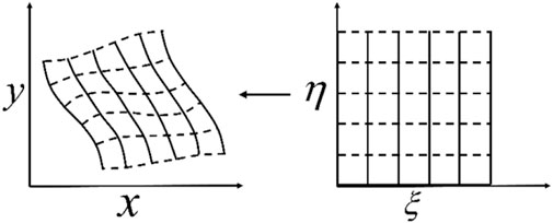
Figure 1. Mapping between the body-fitted grid in the physical domain and the uniform grid in the computational domain.

After the body-fitted grid has been generated, the Cartesian coordinate of each discrete grid points can be determined. Then, the mapping from the curvilinear coordinate to the Cartesian coordinate is

$\begin{array}{l}x=x\left(\xi ,\eta \right)\\ z=z\left(\xi ,\eta \right)\end{array}.(1)$

By taking the partial derivatives of x and y in Equation 1, respectively, we can obtain

$\begin{array}{l}\frac{\partial x}{\partial \xi }\frac{\partial \xi }{\partial x}+\frac{\partial x}{\partial \eta }\frac{\partial \eta }{\partial x}=1\\ \frac{\partial x}{\partial \xi }\frac{\partial \xi }{\partial z}+\frac{\partial x}{\partial \eta }\frac{\partial \eta }{\partial z}=0\\ \frac{\partial z}{\partial \xi }\frac{\partial \xi }{\partial x}+\frac{\partial z}{\partial \eta }\frac{\partial \eta }{\partial x}=0\\ \frac{\partial z}{\partial \xi }\frac{\partial \xi }{\partial z}+\frac{\partial z}{\partial \eta }\frac{\partial \eta }{\partial z}=1\end{array}.(2)$

From Equation 2, we can derive the coefficients of coordinate transformation $\partial \xi /\partial x,\partial \xi /\partial z,\partial \eta /\partial x,\partial \eta /\partial z$:

$\begin{array}{l}\frac{\partial \xi }{\partial x}=\frac{1}{J}\frac{\partial z}{\partial \eta },\frac{\partial \xi }{\partial z}=-\frac{1}{J}\frac{\partial x}{\partial \eta }\\ \frac{\partial \eta }{\partial x}=-\frac{1}{J}\frac{\partial z}{\partial \xi },\frac{\partial \eta }{\partial z}=\frac{1}{J}\frac{\partial x}{\partial \xi }\\ J=\left(\frac{\partial x}{\partial \xi }\frac{\partial z}{\partial \eta }-\frac{\partial x}{\partial \eta }\frac{\partial z}{\partial \xi }\right)\end{array},(3)$

where J is the Jacobian of the transformation and is a non-zero value.

2.2 First-order velocity–stress equations in the curvilinear coordinate

In the pseudo-acoustic VTI media, the first-order velocity–stress pseudo-acoustic wave equation based on first principles is derived by Duveneck et al. (2008):

$\begin{array}{l}\frac{\partial u}{\partial t}=\frac{1}{\rho }\frac{\partial p}{\partial x}\\ \frac{\partial w}{\partial t}=\frac{1}{\rho }\frac{\partial q}{\partial z}\\ \frac{\partial p}{\partial t}=\rho V_p^2\left[\left(1+2\epsilon \right)\frac{\partial u}{\partial x}+\sqrt{1+2\delta }\frac{\partial w}{\partial z}\right]\\ \frac{\partial q}{\partial t}=\rho V_p^2\left[\sqrt{1+2\delta }\frac{\partial u}{\partial x}+\frac{\partial w}{\partial z}\right]\end{array},(4)$

where $u,w$ are components of the particle velocity vector and $p,q$ are the horizontal and vertical stress components, respectively; $\rho$ is the density, $\epsilon ,\delta$ are the Thomsen parameters (Thomsen, 1986); and $V_p$ is the media velocity. These equations can easily be discretized into finite-difference equations on staggered grids. As they have been derived with the acoustic VTI approximation, Equation 4 is kinematically equivalent to acoustic VTI equations derived by Alkhalifah (2000). In addition, one of the advantages of this formulation is the natural handling of variable density.

When the body-fitted grid is applied, Equation 4 should be transformed from the Cartesian coordinate into the curvilinear coordinate. Applying the chain rule, the wave equation in the curvilinear coordinate can be obtained as

$\begin{array}{l}\frac{\partial u}{\partial t}=\frac{1}{\rho }\left(\frac{\partial \xi }{\partial x}\frac{\partial p}{\partial \xi }+\frac{\partial \eta }{\partial x}\frac{\partial p}{\partial \eta }\right)\\ \frac{\partial w}{\partial t}=\frac{1}{\rho }\left(\frac{\partial \xi }{\partial z}\frac{\partial q}{\partial \xi }+\frac{\partial \eta }{\partial z}\frac{\partial q}{\partial \eta }\right)\\ \frac{\partial p}{\partial t}=\rho V_p^2\left[\left(1+2\epsilon \right)\right)\frac{\partial \xi }{\partial x}\frac{\partial u}{\partial \xi }+\sqrt{1+2\delta }\frac{\partial \xi }{\partial z}\frac{\partial w}{\partial \xi }\\ +\left(1+2\epsilon \right)\frac{\partial \eta }{\partial x}\frac{\partial u}{\partial \eta }+\sqrt{1+2\delta }\frac{\partial \eta }{\partial z}\left(\frac{\partial w}{\partial \eta }\right]\\ \frac{\partial q}{\partial t}=\rho V_p^2\left[\sqrt{1+2\delta }\right)\frac{\partial \xi }{\partial x}\frac{\partial u}{\partial \xi }+\frac{\partial \xi }{\partial z}\frac{\partial w}{\partial \xi }+\sqrt{1+2\delta }\frac{\partial \eta }{\partial x}\frac{\partial u}{\partial \eta }+\frac{\partial \eta }{\partial z}\left(\frac{\partial w}{\partial \eta }\right]\end{array},(5)$

where the coefficients of coordinate transformation can be calculated by Equation 3.

2.3 Lebedev grid finite-difference method

In this section, we describe the finite-difference scheme to update Equation 5. The SSG (Virieux, 1986) is widely used to discrete the first-order velocity–stress equation because of its increased stability and ability to suppress numerical dispersion compared with the collocated grid method. However, the velocity and stress in Equation 5 cannot be defined in the staggered-grid points because each variable requires the computation of spatial derivatives in x- and z-directions on the same lattice point. If solving the wave equations using the SSG scheme, some variables need to be calculated by the complex interpolation method, resulting in error and instability. Therefore, we use the LG scheme (Lebedev, 1964) to discretize Equation 5. The way to define LG is shown in Figure 2. The main idea of this grid is that we define different components of velocity (rectangles in Figure 2) and stress (circles in Figure 2) staggered at the same grid points.

Figure 2

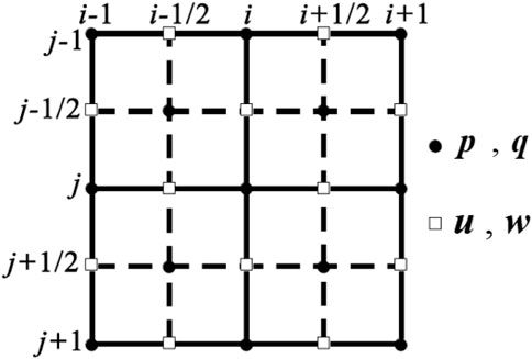
Figure 2. Schematic diagram of the Lebedev grid scheme.

From Figure 2, we can find that the same variable is defined on different locations of the same grid. In addition, every variable requires the computation of spatial derivatives in x- and z-directions on the same grid point. Hence, each variable needs to be calculated separately to update the equation. Taking variableu as an example, we can obtain its discrete form as

$\begin{array}{l}{u}_{i+\frac{1}{2},j}^{n+\frac{1}{2}}=u_{i+\frac{1}{2},j}^{n-\frac{1}{2}}+\frac{\Delta t}{{\rho }_{i+\frac{1}{2},j}}\left[{\left({\xi }_x\right)}_{i+\frac{1}{2},j}{F}_{\xi }{p}_{i+\frac{1}{2},j}^n+{\left({\eta }_x\right)}_{i+\frac{1}{2},j}{F}_{\eta }{p}_{i+\frac{1}{2},j}^n\right]\\ F_{\xi }{p}_{i+\frac{1}{2},j}^n={\displaystyle \sum _{m=1}^L}\frac{c_m}{\Delta \xi }\left[p_{i+\frac{1}{2}+\frac{2m-1}{2},j}^n-p_{i+\frac{1}{2}-\frac{2m-1}{2},j}^n\right]\\ F_{\eta }{p}_{i+\frac{1}{2},j}^n={\displaystyle \sum _{m=1}^L}\frac{c_m}{\Delta \eta }\left[p_{i+\frac{1}{2},j+\frac{2m-1}{2}}^n-p_{i+\frac{1}{2},j-\frac{2m-1}{2}}^n\right]\end{array},(6)$

$\begin{array}{l}{u}_{i,j+\frac{1}{2}}^{n+\frac{1}{2}}=u_{i,j+\frac{1}{2}}^{n-\frac{1}{2}}+\frac{\Delta t}{{\rho }_{i,j+\frac{1}{2}}}\left[{\left({\xi }_x\right)}_{i,j+\frac{1}{2}}{F}_{\xi }{p}_{i,j+\frac{1}{2}}^n+{\left({\eta }_x\right)}_{i,j+\frac{1}{2}}{F}_{\eta }{p}_{i,j+\frac{1}{2}}^n\right]\\ F_{\xi }{p}_{i,j+\frac{1}{2}}^n={\displaystyle \sum _{m=1}^L}\frac{c_m}{\Delta \xi }\left[p_{i+\frac{2m-1}{2},j+\frac{1}{2}}^n-p_{i-\frac{2m-1}{2},j+\frac{1}{2}}^n\right]\\ F_{\eta }{p}_{i,j+\frac{1}{2}}^n={\displaystyle \sum _{m=1}^L}\frac{c_m}{\Delta \eta }\left[p_{i,j+\frac{1}{2}+\frac{2m-1}{2}}^n-p_{i,j+\frac{1}{2}-\frac{2m-1}{2}}^n\right]\end{array},(7)$

where Equation 6 is used to update variable u defined on the grid point (i + 1/2, j) and Equation 7 is used to update variable u defined on the grid point (i, j + 1/2); $\Delta t$ is the time sampling interval, $\Delta \xi$, $\Delta \eta$ is the space sampling interval, and $c_m$ is the finite difference coefficient.

Other variables can be updated by the same way, and then, we can use those discrete equations to simulate wavefields and images. In order to eliminate reflections from the artificial boundary, the sponge absorption boundary condition (Cerjan et al., 1985) is used on the sides and surfaces on top.

2.4 Reverse time migration theory

The realization of the RTM includes three steps. First, the forward propagation of the source wavefield is implemented based on the estimated model parameters, source wavelet, and seismic wave propagation equation. Second, the back propagation of the recorded data at the receiver location used time-reversed wavefield extrapolation operators. Third, the final imaging results are obtained by applying a suitable imaging condition.

The image is formed by multiplying (a zero-lag cross-correlation) the two wavefields at each time step (Claerbout Jon, 1971):

$\text{Image}\left(x,z\right)={\sum }_s{\sum }_t{S}_s\left(x,z,t\right)R_s\left(x,z,t\right),(8)$

where Image, S_s, and R_s represent the imaging result, the wavefield of source, and the wavefield of the receiver, respectively. x and z denote horizontal and depth coordinates, respectively, and t is the time.

The image unit in Equation 8 is amplitude squared; thus, the image magnitude has arbitrary scaling that depends on the source strength and so has no physical interpretation as a reflection coefficient (Chattopadhyay and Mcmechan, 2008).

When compared to the cross-correlation imaging condition, the source-normalized cross-correlation imaging condition yields better imaging amplitudes (Claerbout Jon, 1971; Kaelin and Guitton, 2006). Therefore, we use the source-normalized cross-correlation imaging condition in the form of Equation 9:

$\text{Image}\left(x,z\right)=\frac{{\sum }_s{\sum }_t{S}_s\left(x,z,t\right)R_s\left(x,z,t\right)}{{\sum }_s{\sum }_t{S}_s\left(x,z,t\right)S_s\left(x,z,t\right)}.(9)$

The detail steps of our pseudo-acoustic VTI RTM with surface topography are given in Table 1.

Table 1

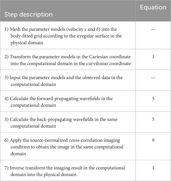
Table 1. Procedural steps for realizing the pseudo-acoustic VTI RTM.

3 Numerical examples

We demonstrate the feasibility of pseudo-acoustic VTI RTM based on the body-fitted grid with synthetic data. The numerical examples are for three models with complex surface topography: 1) a sub-sag model, 2) a modified Hess VTI model, and 3) a modified overthrust VTI model. Forward modeling is the basis of imaging. For better imaging, we suppress shear wave artifacts by a small smoothly tapered circular region with $\epsilon$ set equal to $\delta$ around the source when simulating the wavefield propagation process (Duveneck et al., 2008).

3.1 A sub-sag model

First, we use a sub-sag model with surface topography to examine the accuracy and suitability of the proposed method. The surface of this model is generated with the sinusoidal function: $y=50\sin \left(2\pi /{100}^{*}x\right)+60$. After the body-fitted grid has been generated, the Cartesian coordinate of each discrete grid points and the mapping of coordinate transformation can be used to transform parameter models from the physical domain to the computational domain. Figure 3 shows the model parameters in the physical domain (Figures 3A, C, E) and the computational domain (Figures 3B, D, F). The size of the velocity field was 6,000 m × 3,000 m, with a vertical and horizontal spatial spacing of 10 m. We choose a Ricker wavelet with a 20-Hz peak frequency, and 60 shots are equally distributed at a depth of 10 m, with the distance of 100 m. Each shot has 601 receivers, with an interval of 10 m. The record length is 3.2 s, with a 0.8-ms time sampling interval. From Figures 4A, B, we can see that the generated grid not only has good orthogonality at the boundaries but also maintains good smoothness of the internal grid. This body-fitted grid provides a good basis for the wavefield simulations. Wavefield snapshots at different time steps in the computational domain and the physical domain are shown in Figure 5. As illustrated by the red rectangular box in Figures 5A, C, E, respectively, the shape of the wavefield becomes distorted due to the effects of the undulating surface. In addition, the reflected-wave events in shot records are also distorted, as shown in Figure 6. After transforming the wavefield in the computational to the physical domain (Figures 5B, D, F), the shape of the wavefield is back to normal. All of the snapshots have no numerical dispersion and artificial scattering wave, and the shear wave artifacts are effectively suppressed by loading the source loop. The numerical simulations confirm the accuracy of the LG finite-difference method based on the body-fitted grid. Figure 7 shows the conventional pseudo-acoustic VTI RTM results based on the rectangular grid and the pseudo-acoustic VTI RTM results based on the body-fitted grid. From Figure 7A, we can find that the irregular surface has a serious impact on imaging results. The flat seismic events become distorted, and the tilted seismic events fail to be clearly imaged. In addition, in the shallow region, the imaging results suffer from scattering noise. After considering the influence of subsurface topography in the pseudo-acoustic VTI RTM based on the body-fitted grid, the seismic events are accurately imaged, and the scattering noise is effectively eliminated, as shown in Figure 7B. The results validate that the proposed RTM method has good suitability for the models with complex topographic surfaces.

Figure 3

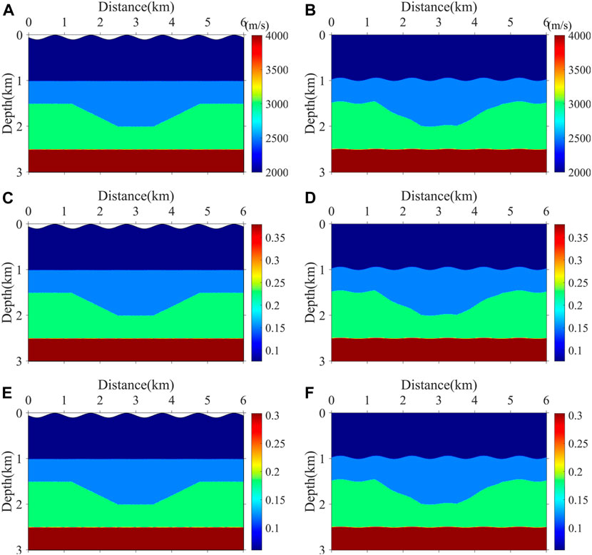
Figure 3. Sub-sag model. (A) Velocity model in the physical domain, (B) velocity model in the computational domain, (C) $\epsilon$ model in the physical domain, (D) $\epsilon$ model in the computational domain, (E) $\delta$ model in the physical domain, and (F) $\delta$ model in the computational domain.

Figure 4

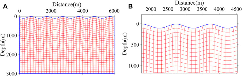
Figure 4. Body-fitted grid. (A) In the physical domain, (B) zoomed views of (A).

Figure 5

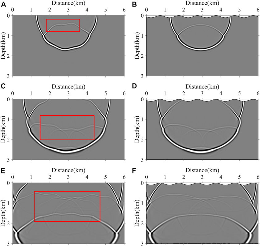
Figure 5. Wavefield snapshots at different time steps. (A,C,E) t = 800 ms, t = 1,120 ms, and t = 1,440 ms, respectively, in the computational domain; (B,D,F) t = 800 ms, t = 1,120 ms, and t = 1,440 ms, respectively, in the physical domain.

Figure 6

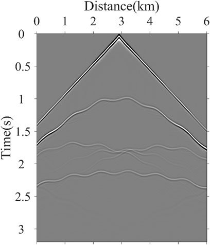
Figure 6. 30th shot records.

Figure 7

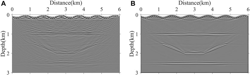
Figure 7. RTM imaging results in the physical domain. (A) Conventional pseudo-acoustic VTI RTM based on the rectangular grid and (B) pseudo-acoustic VTI RTM based on the body-fitted grid.

3.2 A modified Hess VTI model

We use the modified Hess VTI model with complex surfaces for imaging to verify the reliability of our pseudo-acoustic VTI RTM algorithm in complex models. Figure 8 shows the velocity and the anisotropic parameters of the Hess model in the physical domain (Figures 8A, C, E) and computational domain (Figures 8B, D, F). The model has a high-speed salt dome structure and a fault structure, and it has a strong anisotropic characteristic. The surface of this model is generated by the function: $y=75\sin \left(2\pi /150*x\right)+100$. The grid size of the model is 901 × 425, with a vertical and horizontal spatial spacing of 10 m. The time sampling interval of numerical simulation is 0.8 ms, and the total record length is 4.0 s. A Ricker wavelet with a 20-Hz dominant frequency is excited as the source wavelet. There are 90 shots at a depth of 10 m with a 100-m spacing interval and 901 receivers with a 10-m spacing interval. From the wavefield snapshots (Figures 9A, B) and the shot records (Figures 10A, B), we conclude that the seismic waves simulated with our method can propagate stably in complex media with complex subsurface topography. We perform the conventional pseudo-acoustic VTI RTM based on the rectangular grid, the ISO RTM, and the pseudo-acoustic VTI RTM based on the body-fitted grid on the synthetic dataset, and the obtained imaging results are shown in Figure 11. From Figure 11A, it is clear that the seismic events in the shallow region are hard to be recognized because they are covered by scattering noise. In addition, the seismic events in other regions have poor contiguity. Compared with Figure 11A, the results in Figure 11C show that the proposed RTM method can effectively suppress scattering noise and produce clearer and more accurate images than conventional pseudo-acoustic VTI RTM based on the rectangular grid. As shown in the black rectangular box in Figure 11B, there is an obvious non-convergence of diffracted waves in the area of strong anisotropy because the anisotropy is ignored in ISO RTM. The same region in Figure 11C is well-imaged after considering the effect of the anisotropy. In addition, diffraction waves generated by the fault plane do not converge well, which is denoted by the red ellipse box in Figure 11B, while the fault plane in Figure 11C is well-imaged. In general, the seismic events are more detailed and clearer, and the total resolution is significantly improved in the pseudo-acoustic VTI RTM results. This experiment demonstrates that the pseudo-acoustic VTI RTM based on the body-fitted grid produces more accurate and higher-resolution imaging results.

Figure 8

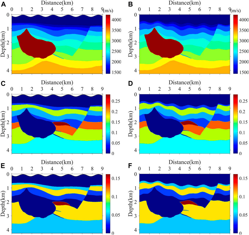
Figure 8. Modified Hess VTI model. (A) Velocity model in the physical domain, (B) velocity model in the computational domain, (C) $\epsilon$ model in the physical domain, (D) $\epsilon$ model in the computational domain, (E) $\delta$ model in the physical domain, and (F) $\delta$ model in the computational domain.

Figure 9

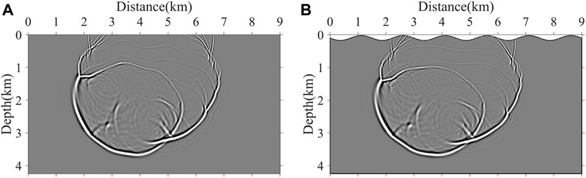
Figure 9. Wavefield snapshots at 1,600 ms. (A) Snapshots in the computational domain and (B) snapshots in the physical domain.

Figure 10

Figure 10. Shot records. (A) 45th shot records and (B) 60th shot records.

Figure 11

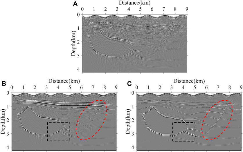
Figure 11. RTM imaging results in the physical domain. (A) Conventional pseudo-acoustic VTI RTM based on the rectangular grid, (B) ISO RTM based on the body-fitted grid, and (C) pseudo-acoustic VTI RTM based on the body-fitted grid.

3.3 A modified overthrust VTI model

To further validate the applicability of our method to complex models, we modified the overthrust VTI model. The velocity and the anisotropic parameters of the modified overthrust model in the physical domain (Figures 12A, C, E) and computational domain (Figures 12B, D, F) are shown in Figure 12. The model has a lot of overthrust faults and high-steep structures, which have a strongly anisotropic characteristic. The irregular subsurface is generated according to the first-layer interface of the model, which is more general in nature. The grid size of the model is 751 × 371, with a vertical and horizontal spatial spacing of 10 m. The time sampling interval of numerical simulation is 0.5 ms, and the total record length is 3.0 s. A Ricker wavelet with a 25-Hz dominant frequency is excited as the source wavelet. There are 75 shots at a depth of 10 m with a 100-m spacing interval and 751 receivers with a 10-m spacing interval. As shown by the yellow arrows in Figure 13A, there is an obvious non-convergence of diffracted waves, which results in the failure to image the deep fold structure because the anisotropy is ignored in ISO RTM. The same region shown in Figure 13B is well-imaged after considering the effect of the anisotropy. In addition, diffraction waves generated by the overthrust fault plane do not converge well, which is denoted by the red arrows, as shown in Figure 13A, while the fault plane, as shown in Figure 13B, is well-imaged. In general, the imaging results, as shown in Figure 13B, have higher signal-to-noise ratios and higher resolution.

Figure 12

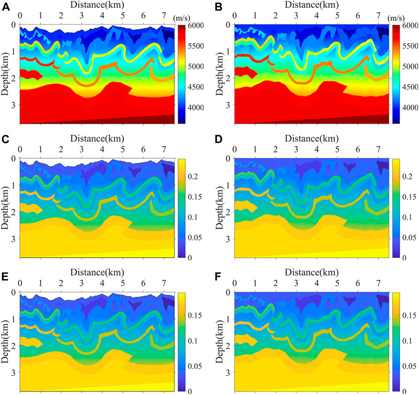
Figure 12. Modified overthrust VTI model. (A) Velocity model in the physical domain, (B) velocity model in the computational domain, (C) $\epsilon$ model in the physical domain, (D) $\epsilon$ model in the computational domain, (E) $\delta$ model in the physical domain, and (F) $\delta$ model in the computational domain.

Figure 13

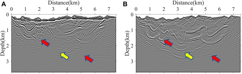
Figure 13. RTM imaging results in the physical domain. (A) ISO RTM based on the body-fitted grid and (B) pseudo-acoustic VTI RTM based on the body-fitted grid.

4 Discussion

To avoid the artificial scattering waves due to the staircase discretization of the irregular surface, we use the body-fitted grid to discretize the computational domain. This grid has interior smoothness and local orthogonality at the boundary, as shown in Figure 4, and it can easily conform to the irregular surface. Since the finite difference scheme is implemented in the curvilinear coordinate, the standard-staggered grid (SSG) finite difference scheme is no longer applicable, so we use the LG scheme (Lebedev, 1964) to update Equation 5. The numerical simulations in the sub-sag model and the Hess VTI model validate the accuracy of the LG finite difference method based on the body-fitted grid.

To validate the applicability of the proposed RTM method, we use three numerical tests on the models with different irregular surfaces. Although the third model includes a dramatically undulating surface, all correct imaging results of the models validate the advantages of the proposed method for dealing with various undulating surfaces. In addition, we use the ISO RTM and pseudo-acoustic VTI RTM methods to process the simulated dataset. All these results indicate that the pseudo-acoustic VTI RTM based on the body-fitted grid can solve the effect of anisotropy and complex surface topography on seismic wave propagation and get clearer and more accurate subsurface images.

When comparing Equation 4 and Equation 5, we can find that the equations in the curvilinear coordinate include additional derivative terms that are not present in the Cartesian coordinate. Although the finite difference scheme based on the body-fitted grid in the curvilinear coordinate has better simulation accuracy, it requires more computation costs and memory overhead, which will also lead to a decrease in imaging efficiency. Therefore, further improvement of this method is to provide a reasonable balance between numerical accuracy and computational efficiency.

5 Conclusion

We develop a pseudo-acoustic VTI RTM method based on the body-fitted grid for anisotropic shot data with complex surface topography. The orthogonal body-fitted grid can well fit the irregular surface, which can avoid artificial scattering waves in the propagation of the wavefield. Based on the coordinate transformation, we derive a first-order velocity–stress pseudo-acoustic wave equation in the curvilinear coordinate system. The LG finite-difference method is used to solve the first-order equation, which can avoid complex interpolation calculations and improve the accuracy and stability of the simulation. After considering the impact of the non-flat surface and anisotropy, the proposed RTM method can produce correct travel times during source and receiver wavefield extrapolation and obtain accurate and high-quality imaging results. Numerical examples demonstrate the feasibility and robustness of the proposed method for the pseudo-acoustic VTI media with complex surface topography.

Data availability statement

The original contributions presented in the study are included in the article/Supplementary Material; further inquiries can be directed to the corresponding author.

Author contributions

EW: conceptualization, data curation, formal analysis, investigation, methodology, software, validation, visualization, writing–original draft, writing–review and editing, and resources. JH: funding acquisition, investigation, methodology, software, and writing–review and editing. ZL: formal analysis, methodology, supervision, and writing–review and editing. XM: investigation, methodology, software, and writing–review and editing. QL: methodology, software, and writing–review and editing.

Funding

The authors declare that financial support was received for the research, authorship, and/or publication of this article. This study is supported by the Major Scientific and Technological Projects of Shandong Energy Group (no. SNKJ 2022A06-R23), the Marine S&T Fund of Shandong Province for the Pilot National Laboratory for Marine Science and Technology (Qingdao) (no. 2021QNLM020001), the Funds of Creative Research Groups of China (no. 41821002), the Natural Science Foundation of Shandong Province-General Program (no. ZR2023MD087), and the Basic Theoretical Research of Seismic Wave Imaging Technology in Complex Oilfield of Changqing Oilfield Company (no. 2023–10502). The funder was not involved in the study design, collection, analysis, interpretation of data, the writing of this article, or the decision to submit it for publication.

Acknowledgments

The authors would like to thank all members of the seismic inversion and imaging group of China University of Petroleum (East China) for their comments and discussions. They would also like to thank the reviewers and the editorial department for their constructive and thoughtful comments and suggestions, which greatly improved the quality of this study.

Conflict of interest

Author LQ was employed by Sinopec Zhongyuan Oilfield Company.

The remaining authors declare that the research was conducted in the absence of any commercial or financial relationships that could be construed as a potential conflict of interest.

Publisher’s note

All claims expressed in this article are solely those of the authors and do not necessarily represent those of their affiliated organizations, or those of the publisher, the editors, and the reviewers. Any product that may be evaluated in this article, or claim that may be made by its manufacturer, is not guaranteed or endorsed by the publisher.

References

Alkhalifah, T. (1998). Acoustic approximations for processing in transversely isotropic media. Geophysics 63, 623–631. doi:10.1190/1.1444361

CrossRef Full Text | Google Scholar

Alkhalifah, T. (2000). An acoustic wave equation for anisotropic media. Geophysics 65, 1239–1250. doi:10.1190/1.1444815

CrossRef Full Text | Google Scholar

Appelö, D., and Petersson, N. A. (2009). A stable finite difference method for the elastic wave equation on complex geometries with free surfaces. Commun. Comput. Phys. 4, 84–107. doi:10.2140/camcos.2009.4.217

CrossRef Full Text | Google Scholar

Baysal, E., D.Kosloff, D., and Sherwood, W. C. (1983). Reverse time migration. Geophysics 48, 1514–1524. doi:10.1190/1.1441434

CrossRef Full Text | Google Scholar

Beasley, C., and Lynn, W. (1992). The zero-velocity layer; migration from irregular surfaces. Geophysics 57, 1435–1443. doi:10.1190/1.1443211

CrossRef Full Text | Google Scholar

Berryhill, J. R. (1979). Wave-equation datuming. Geophysics 44, 1329–1344. doi:10.1190/1.1441010

CrossRef Full Text | Google Scholar

Bevc, K. (1997). Flooding the topography: wave-equation datuming of land data with rugged acquisition topography. Geophysics 62, 1558–1569. doi:10.1190/1.1444258

CrossRef Full Text | Google Scholar

Cerjan, C., Kosloff, D., Kosloff, R., and Reshef, M. (1985). A nonreflecting boundary condition for discrete acoustic and elastic wave equations. Geophysics 50, 705–708. doi:10.1190/1.1441945

CrossRef Full Text | Google Scholar

Chattopadhyay, S., and McMechan, G. A. (2008). Imaging conditions for prestack reverse-time migration. Geophysics 73, S81–S89. doi:10.1190/1.2903822

CrossRef Full Text | Google Scholar

Chu, C., Macy, B. K., and Anno, P. D. (2011). Approximation of pure acoustic seismic wave propagation in TTI media. Geophysics 76, WB97–WB107. doi:10.1190/geo2011-0092.1

CrossRef Full Text | Google Scholar

Claerbout Jon, F. (1971). Toward a unified theory of reflector mapping. Geophysics 36, 467–481. doi:10.1190/1.1440185

CrossRef Full Text | Google Scholar

de la Puente, J., Ferrer, M., Hanzich, M., Castillo, J. E., and Cela, J. M. (2014). Mimetic seismic wave modeling including topography on deformed staggered grids. Geophysics 79, T125–T141. doi:10.1190/geo2013-0371.1

CrossRef Full Text | Google Scholar

Duveneck, E., and Bakker, P. M. (2011). Stable P-wave modeling for reverse-time migration in tilted TI media. Geophysics 76, S65–S75. doi:10.1190/1.3533964

CrossRef Full Text | Google Scholar

Duveneck, E., Milcik, P., Bakker, P. M., and Perkins, C. (2008). Acoustic VTI wave equations and their application for anisotropic reverse-time migration. 78th Annu. Int. Meet. Seg. Expand. Abstr., 2186–2190. doi:10.1190/1.3059320

CrossRef Full Text | Google Scholar

Fletcher, R. P., Du, X., and Fowler, P. J. (2009). Reverse time migration in tilted transversely isotropic (TTI) media. Geophysics 74, WCA179–WCA187. doi:10.1190/1.3269902

CrossRef Full Text | Google Scholar

Fornberg, B. (1988). The pseudospectral method: accurate representation of interfaces in elastic wave calculations. Geophysics 53, 625–637. doi:10.1190/1.1442497

CrossRef Full Text | Google Scholar

Fowler, P. J., Du, X., and Fletcher, R. P. (2010). Coupled equations for reverse time migration in transversely isotropic media. Geophysics 75, S11–S22. doi:10.1190/1.3294572

CrossRef Full Text | Google Scholar

Hayashi, K., Burns, D. R., and Toksöz, M. N. (2001). Discontinuous-grid finite-difference seismic modeling including surface topography. Bull. Seismol. Soc. Am. 91, 1750–1764. doi:10.1785/0120000024

CrossRef Full Text | Google Scholar

Hestholm, S., and Ruud, B. (1994). 2D finite-difference elastic wave modelling including surface topography1. Geophys. Prospect. 42, 371–390. doi:10.1111/j.1365-2478.1994.tb00216.x

CrossRef Full Text | Google Scholar

Kaelin, B., and Guitton, A. (2006). Imaging condition for reverse time migration. 76th Annu. Int. Meet. Expo. Seg. Expand. Abstr., 2594–2598. doi:10.1190/1.2370059

CrossRef Full Text | Google Scholar

Konuk, T., and Shragge, J. (2021). Tensorial elastodynamics for anisotropic media. Geophysics 86, T293–T303. doi:10.1190/geo2020-0156.1

CrossRef Full Text | Google Scholar

Lan, H. Q., Zhang, Z. J., Chen, J. Y., and Liu, Y. S. (2014). Reverse time migration from irregular surface by flattening surface topography. Tectonophysics 627, 26–37. doi:10.1016/j.tecto.2014.04.015

CrossRef Full Text | Google Scholar

Lebedev, V. I. (1964). Difference analogues of orthogonal decompositions of basic differential operators and some boundary value problems. I. USSR Comput. Math. Math. Phys. 4, 449–465. doi:10.1016/0041-5553(64)90240-x

CrossRef Full Text | Google Scholar

Liu, F., Morton, S. A., Jiang, S., Ni, L., and Leveille, J. P. (2009). Decoupled wave equations for P and SV waves in an acoustic VTI media. 79th Annu. Int. Meet. Seg. Expand. Abstr., 2844–2848. doi:10.1190/1.3255440

CrossRef Full Text | Google Scholar

Mcmechan, G. A. (1983). Migration by extrapolation of time-dependent boundary values. Geophys. Prospect. 31, 413–420. doi:10.1111/j.1365-2478.1983.tb01060.x

CrossRef Full Text | Google Scholar

Mu, X., Huang, J., Li, Z., Liu, Y., Su, L., and Liu, J. (2022). Attenuation compensation and anisotropy correction in reverse time migration for attenuating tilted transversely isotropic media. Surv. Geophys. 43, 737–773. doi:10.1007/s10712-022-09707-2

CrossRef Full Text | Google Scholar

Mu, X., Huang, J., Mao, Q., and Han, J. (2023). Efficient pure qP-wave simulation and reverse time migration imaging for vertical transverse isotropic (VTI) media. J. Geophys. Eng. 20, 712–722. doi:10.1093/jge/gxad039

CrossRef Full Text | Google Scholar

Mu, X., Huang, J., Yang, J., Guo, X., and Guo, Y. (2020a). Least-squares reverse time migration in TTI media using a pure qP-wave equation. Geophysics 85, S199–S216. doi:10.1190/geo2019-0320.1

CrossRef Full Text | Google Scholar

Mu, X., Huang, J., Yong, P., Huang, J., Guo, X., Liu, D., et al. (2020b). Modeling of pure qP- and qSV-waves in tilted transversely isotropic media with the optimal quadratic approximation. Geophysics 85, C71–C89. doi:10.1190/geo2018-0460.1

CrossRef Full Text | Google Scholar

Ohminato, T., and Chouet, B. A. (1997). A free-surface boundary condition for including 3D topography in the finite-difference method. Bull. Seismol. Soc. Am. 87, 494–515. doi:10.1785/bssa0870020494

CrossRef Full Text | Google Scholar

Qu, Y., Huang, J., Li, Z., and Li, J. (2017). A hybrid grid method in an auxiliary coordinate system for irregular fluid–solid interface modelling. Geophys. J. Int. 208, 1540–1556. doi:10.1093/gji/ggw429

CrossRef Full Text | Google Scholar

Qu, Y. M., and Li, J. L. (2019). Q-compensated reverse time migration in viscoacoustic media including surface topography. Geophysics 84, S201–S217. doi:10.1190/geo2018-0313.1

CrossRef Full Text | Google Scholar

Reshef, M. (1991). Depth migration from irregular surfaces with depth extrapolation methods. Geophysics 56, 119–122. doi:10.1190/1.1442947

CrossRef Full Text | Google Scholar

Robertsson, J. O. A. (1996). A numerical free-surface condition for elastic/viscoelastic finite-difference modeling in the presence of topography. Geophysics 61, 1921–1934. doi:10.1190/1.1444107

CrossRef Full Text | Google Scholar

Sethi, H., Shragge, J., and Tsvankin, I. (2022). Tensorial elastodynamics for coupled acoustic/elastic anisotropic media: incorporating bathymetry. Geophys. J. Int. 228, 999–1014. doi:10.1093/gji/ggab374

CrossRef Full Text | Google Scholar

Tarrass, I., Giraud, L., and Thore, P. (2011). New curvilinear scheme for elastic wave propagation in presence of curved topography. Geophys. Prospect. 59, 889–906. doi:10.1111/j.1365-2478.2011.00972.x

CrossRef Full Text | Google Scholar

Tessmer, E., Koslof, D., and andBehle, A. (1992). Elastic wave propagation simulation in the presence of surface topography. Geophys. J. Int. 108, 621–632. doi:10.1111/j.1365-246x.1992.tb04641.x

CrossRef Full Text | Google Scholar

Thomsen, L. (1986). Weak elastic anisotropy. Geophysics 51, 1954–1966. doi:10.1190/1.1442051

CrossRef Full Text | Google Scholar

Virieux, J. (1986). P-SV wave propagation in heterogeneous media: velocity-stress finite-difference method. Geophysics 51, 889–901. doi:10.1190/1.1442147

CrossRef Full Text | Google Scholar

Zhan, G., Pestana, R. C., and Stoffa, P. L. (2012). Decoupled equations for reverse time migration in tilted transversely isotropic media. Geophysics 77, T37–T45. doi:10.1190/geo2011-0175.1

CrossRef Full Text | Google Scholar

Zhang, W., and Chen, X. F. (2006). Traction image method for irregular free surface boundaries in finite difference seismic wave simulation. Geophys. J. Int. 167, 337–353. doi:10.1111/j.1365-246X.2006.03113.x

CrossRef Full Text | Google Scholar

Zhang, Y., Zhang, H., and Zhang, G. (2011). A stable TTI reverse time migration and its implementation. Geophysics 76, WA3–WA11. doi:10.1190/1.3554411

CrossRef Full Text | Google Scholar

Zhou, H., Zhang, G., and Bloor, R. (2006a). “An anisotropic acoustic wave equation for VTI media,” in 68th Annual International Conference and Exhibition, EAGE, Extended Abstracts, China, 08 August 2022. doi:10.3997/2214-4609.201402310

CrossRef Full Text | Google Scholar