 Céline Martin
 Nora Richter2
 Linda Amaral-Zettler
 Nathalie Dubois
- 1Eawag, Surface Waters Research + Management, Dübendorf, Switzerland
- 2NIOZ Royal Netherlands Institute for Sea Research, Department of Marine Microbiology and Biogeochemistry, Den Burg, Netherlands
- 3Institute for Biodiversity and Ecosystem Dynamics, Department of Freshwater and Marine Ecology, University of Amsterdam, Amsterdam, Netherlands
Lacustrine alkenones are increasingly reported in freshwater lakes worldwide, which makes them a very promising proxy to reconstruct past continental temperatures. However, a more systematic understanding of ecological preferences of freshwater alkenone-producers at global scale is lacking, which limits our understanding of alkenones as a proxy in lakes. Here we investigated 56 Swiss freshwater lakes and report Group 1 alkenones in 33 of them. In twelve of the lakes containing alkenones, a mixed Group 1/Group 2 alkenone signature was detected. We used a random forest (RF) model to investigate the influence of 15 environmental variables on alkenone occurrence in Swiss lakes and found sodium (Na+) concentration and mean annual air temperature (MAAT) to be the most important variables. We also trained a RF model on a database that included Swiss lakes and all freshwater lakes worldwide, which were previously investigated for alkenone presence. Water depth appeared as the most important variable followed by MAAT and Na+, sulfate and potassium concentrations. This is very similar to results found for freshwater and saline lakes, which suggests that Group 1 and Group 2 alkenone occurrence could be controlled by the same variables in freshwater lakes. For each tested variable, we defined the optimal range(s) for the presence of alkenones in freshwater lakes. The similarity of the results for the Swiss and global models suggests that the environmental parameters controlling the occurrence of freshwater alkenone producers could be homogenous worldwide.
1 Introduction
Alkenones are a class of C35 to C42 methyl (Me) and ethyl (Et) ketones, with 2–4 double bonds, only produced by haptophyte algae of the order Isochrysidales. They are ubiquitous in the world’s oceans (e.g., de Leeuw et al., 1980; Conte et al., 2006) and have been found in various lake environments (e.g., Zink et al., 2001; Chu et al., 2005; D’Andrea and Huang, 2005; Pearson et al., 2008; Longo et al., 2016; 2018). The degree of unsaturation of alkenones is known to reflect algal growth temperatures (Brassell et al., 1986; Prahl and Wakeham, 1987) and the C37 alkenone unsaturation indices (
Alkenone producing Isochrysidales were divided into three phylogenetically distinct groups (Theroux et al., 2010): Group 1, occurring in freshwater and oligohaline lakes, Group 2, in brackish waters and saline lakes, coastal seas and/or sea ice environments, and Group 3 in open ocean environments (e.g., Theroux et al., 2010; Toney et al., 2012; Longo et al., 2016; Araie et al., 2018; Wang et al., 2021). Group 1 Isochrysidales were divided into two subclades (Richter et al., 2019): Group 1a (formerly “Greenland” subclade; D’Andrea et al., 2006) and Group 1b (formerly ‘‘EV” subclade; Simon et al., 2013). While Group 2 Isochrysidales contains three subclades: Groups 2i and 2w1, mainly occurring in lakes with relatively low to intermediate salinity and Group 2w2, preferring to occur in hypersaline lakes (Wang et al., 2021; Yao et al., 2022). Group 2i is associated with ice and Groups 2w1 and 2w2 bloom during the warm season (Wang et al., 2021; Yao et al., 2022). Despite the genetic diversity of Group 1 Isochrysidales, Group 1 alkenones seem to be immune to species-mixing effects, making them an ideal tool for quantitative paleotemperature reconstructions on continents (Wang et al., 2022). They have been successfully applied in high- and mid-latitude freshwater lakes to reconstruct past temperatures (e.g., D’Andrea et al., 2011; D’Andrea et al., 2012; Longo et al., 2020; Richter et al., 2021b; Yao et al., 2023b; Yao et al., 2023a).
Unlike Group 3 Isochrysidales, lacustrine Isochrysidales are not present in all lakes (e.g., Brassell et al., 2022). So far, Group 1 Isochrysidales have not been successfully isolated for laboratory culture. Therefore, we can only rely on environmental studies to better understand their ecological preferences. Several studies tried to understand which parameters could influence alkenone occurrence in lakes comparing lakes with and without alkenones in Europe (Cranwell, 1985; Zink et al., 2001; Pearson et al., 2008), Asia (Chu et al., 2005; Liu et al., 2011; Zhao et al., 2014; McColl, 2016; Song et al., 2016; Yao et al., 2019; He et al., 2020; Yao et al., 2021; Yao et al., 2022; Bulkhin et al., 2023), North America (Toney et al., 2010; Toney et al., 2011; Longo et al., 2016; Plancq et al., 2018a), Greenland (D’Andrea and Huang, 2005; D’Andrea et al., 2011) and globally distributed lakes (Longo et al., 2018). Simple comparisons, principal component analysis (PCA) or logistic regressions were used to determine which environmental factors might influence alkenone occurrence and abundance in the various datasets. Plancq et al. (2018a) was the first study to use a model - a binomial regression model, member of the family of generalized linear models - which allowed the authors to test and compare the importance of several variables for alkenone occurrence and abundance. They found salinity, water temperature, lake depth, stratification and pH to be the main controls of alkenone occurrence in 106 Canadian prairie lakes, including mainly saline lakes. However, very few of these studies focused on freshwater lakes. As freshwater and saline lakes do not host the same Isochrysidales groups, the parameters influencing the occurrence of Group 1 in freshwater lakes and Group 2 in saline lakes could be different. Moreover, all studies, so far, were focused on a specific region with limited ranges for some environmental variables.
Here we investigate alkenone occurrence and producer diversity in 56 Swiss freshwater lakes for which numerous environmental data was collected. To assess which environmental variables control the occurrence of alkenones in Swiss lakes, we use a new approach based on a type of machine learning, random forest (RF, Breiman, 2001). With this non-linear model, we seek to identify the best predictors of alkenone occurrence in Swiss lakes. We combine our data with all previous data available on presence/absence of alkenones in global freshwater lakes (total number of 396 lakes) and compare the results obtained with the models trained exclusively with Swiss lakes and with both Swiss and global lakes. The RF model assesses the importance of each environmental variable for the prediction of alkenone occurrence. Investigating these statistical relationships can help reveal biological mechanisms and thus, improve our understanding of the ecological preferences for Isochrysidales.
2 Material and methods
2.1 Sites and sampling
For this study, 56 freshwater lakes were studied: 55 Swiss lakes and one in France, close to the border with Switzerland (Figure 1A; Table 1). Surface sediments were collected between 2011 and 2020 with a gravity corer from the deepest point in the lake, whenever possible. The cores were stored at 4°C until sampling.
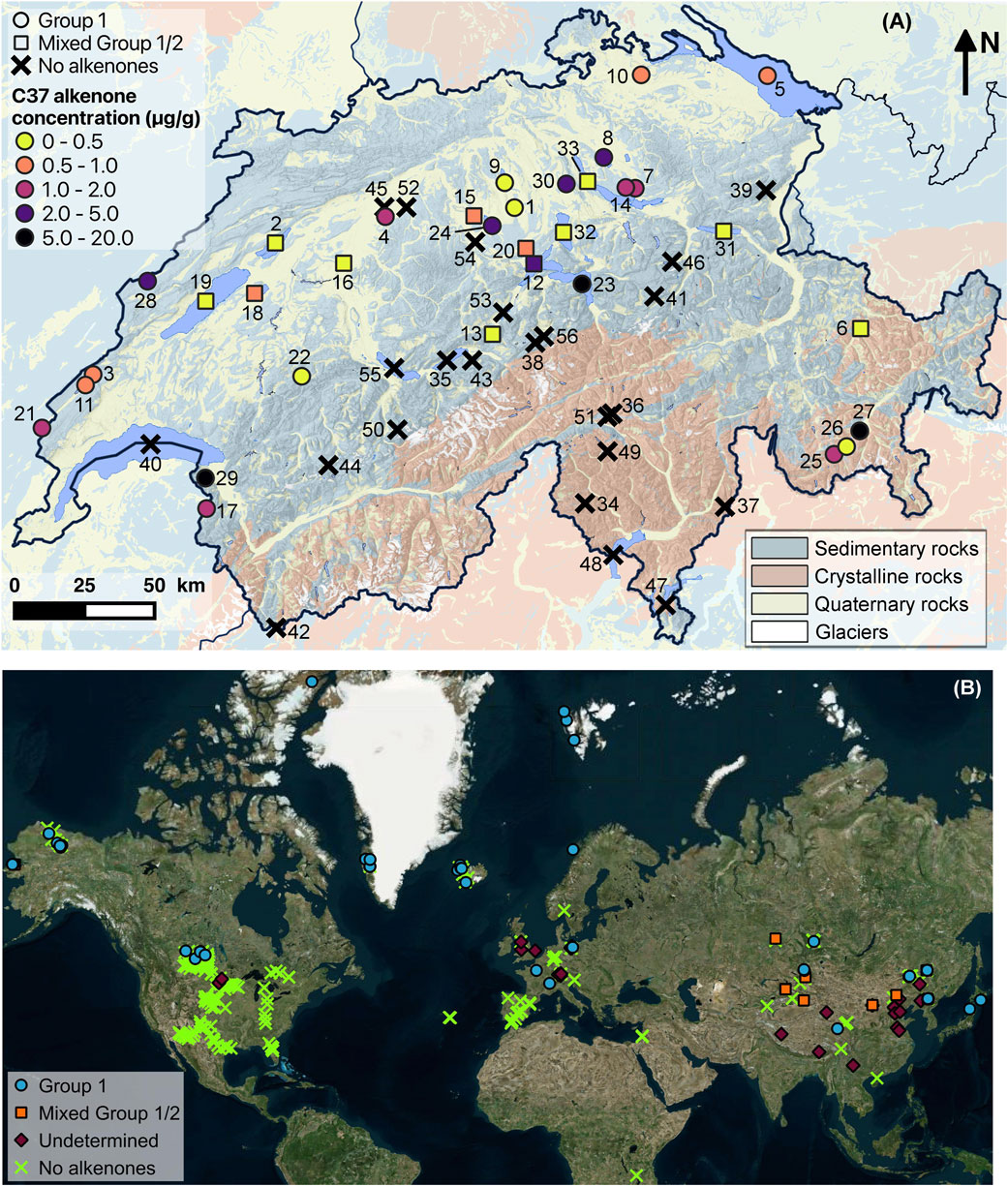
Figure 1. Maps showing the location of the studied Swiss lakes and the lakes from the global database. (A) Lakes containing Group 1 alkenones in their surface sediments are indicated by circles, those containing both Group 1 and Group 2 alkenones by squares, while those without alkenones are represented by black crosses. The color of the symbols represents the alkenone concentration. Numbers correspond to lakes listed in Table 1. The relief and the main geological zones are shown in the background (maps from SwissTopo and the Georesources Switzerland Group). (B) Map showing the distribution of the freshwater lakes from the global database with Group 1 (blue circle), mixed Group 1/2 (orange square) or undetermined group of Isochrysidales (purple diamond). Lakes without alkenones are indicated by green crosses. Data for global freshwater lakes are from Cranwell (1985), Innes et al. (1998), Zink et al. (2001), Huang et al. (2004), Chu et al. (2005), D’Andrea and Huang (2005), D’Andrea et al. (2006), D’Andrea et al. (2012), D’Andrea et al. (2016), de Mesmay et al. (2007), Hou et al. (2008), Pearson et al. (2008), Toney et al. (2010, 2011), Liu et al. (2011), Simon et al. (2013), Simon et al. (2015), Hou et al. (2016), Longo et al. (2016), Longo et al. (2018), McColl (2016), Song et al. (2016), Plancq et al. (2018a), Plancq et al. (2018b), Plancq et al. (2019), van der Bilt et al. (2018), Wang et al. (2019), Yao et al. (2019), Yao et al. (2021), Yao et al. (2022), Yao et al. (2023b), Harning et al. (2020), He et al. (2020), Schroeter et al. (2020), Raja et al. (2022), Cluett et al. (2023), Bulkhin et al. (2023) and Krivonogov et al. (2023).
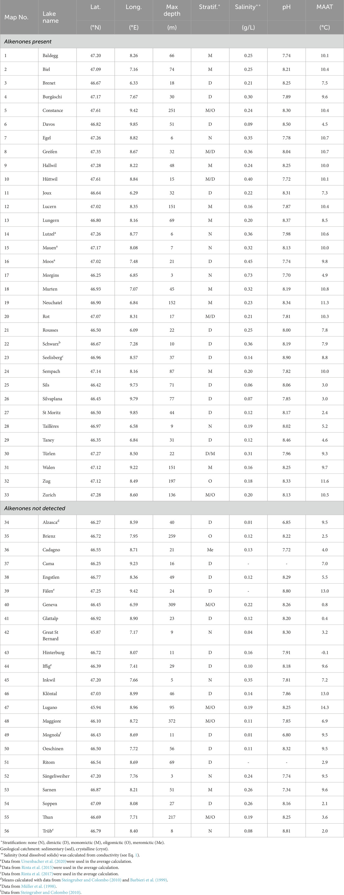
Table 1. Location and physico-chemical parameters of the surface waters (0–15 m) of the studied Swiss lakes. When possible, the average of the 10 years preceding the coring was calculated.
The geographic characteristics of the studied lakes span a wide-range of physical gradients, including an altitudinal gradient from 193 to 2,447 m, maximal depth from 3 to 372 m and mean annual air temperature (MAAT) from −0.1°C to 14.3°C (Table 1; Supplementary Table S1). Lakes were sampled in the two main geological ensembles of Switzerland: the Swiss Plateau, Jura mountains and the external zone of the Alps, covered with sedimentary rocks, and the internal zone of the Alps, characterized by crystalline bedrock (Figure 1A; Supplementary Table S1).
2.2 Environmental parameters
The physico-chemical parameters of the surface waters (0–15 m) of the Swiss lakes (Table 1; Supplementary Table S1) are from long-term monitoring projects conducted by the environmental agencies of Swiss cantons and by Eawag (www.datalakes-eawag.ch). Data was obtained from the Naïade database (naiades.eaufrance.fr) for the French lake, Lac des Rousses. Data for Lake Constance have been provided by the Bodensee-Wasserinformationssystem (BOWIS) database, which is managed by the Internationalen Gewasserschutzkommission fur den Bodensee (IGKB). The data for Lake Lugano was provided by the International Commission for the Protection of Italian-Swiss Waters (CIPAIS, www.cipais.org). When data was not available, we measured pH, conductivity and oxygen concentration with a WTW multi-parameter sonde at 0.5 m and we sampled 1 L of water at 0.5 m below the surface to measure major ions and trace elements. Water temperatures were not available for all lakes, so we used mean annual air temperatures from the closest MeteoSwiss meteorological stations and corrected for any altitudinal difference applying a lapse rate of 0.6°C/100 m (Gandouin et al., 2016). When possible, a mean of the 10 years preceding the coring was calculated for all physico-chemical parameters and MAAT, assuming that 1 cm of sediment integrates on average 10 years of sedimentation (Supplementary Table S2).
Salinity was equated to the total dissolved solids (TDS), which was calculated from conductivity using the equation from Pawlowicz and Feistel (2012):
where TDS is expressed in mg/kg, which corresponds to mg/L in freshwater lakes, and
The mixing regime of lakes was deduced from long-term water temperature monitoring, modeling (simstrat.eawag.ch) and the literature. When the stratification status was unknown, we deduced it using the following method: for each lake, we calculated the thermocline depth from lake area according to Hanna (1990), (Eq. 2) and we compared the resulting thermocline depth with the actual depth of the lake. If the depth of the lake was at least 2 m deeper than the calculated thermocline depth, we classified the lake as stratified.
where
For each lake, the geological catchment was classified as sedimentary or crystalline using the Swiss geological map provided by SwissTopo and the Georesources Switzerland Group (map.geo.admin.ch). When lakes had both sedimentary and crystalline rocks in their catchment, they were attributed to the class of the dominant rock type.
2.3 Global database
In order to compare the results found in Swiss lakes with previous results from the literature, we collected all the data available on global freshwater lakes investigated for alkenone presence and constructed a global database (Figure 1B; Supplementary Table S3). We only considered surface or subsurface sediments. When salinity data was available, we used a limit of 3 g/L; Lake Little Manitou (Canada) and Yarkov basin of Chany Lake (Russia) exceeded this limit (salinity of 3.62 and 7.1 g/L, respectively) but were included in the database as the alkenone distribution indicated the presence of Group 1 alkenones (Plancq et al., 2018a; Krivonogov et al., 2023). Otherwise, we selected lakes classified as fresh. All lakes only containing Group 2 alkenones were excluded. The database includes 340 lakes globally distributed, among which 103 lakes contain alkenones: 67 host Group 1 alkenones including 32 where Group 1 was genetically confirmed, 10 host a mix of Group 1/2 alkenones including 3 where the mixing was genetically confirmed (Figure 1B; Supplementary Table S3). For the remaining 26 lakes, it was not possible to determine which alkenone group was present. However, as the probability of Group 1 presence is very high for lakes with salinities lower than 6 g/L (Yao et al., 2020), it is likely that they host Group 1 alkenones or a mix of Group 1/2. The WorldClim database (Fick and Hijmans, 2017) was used to provide MAAT when it was not provided. We used the method described above to deduce the stratification status when it was not mentioned.
2.4 Sample preparation
For each lake, the top 0–1 or 1–2 cm sediments were sampled and freeze-dried. 1–5 g of sediments were ground and homogenized before extraction with an accelerated solvent extraction system ASE350 (Dionex) with dichloromethane:methanol (DCM:MeOH 9:1, v:v) at 120°C and 1,200 psi. The total lipid extracts (TLEs) were split in two equal parts. One part was saponified by adding 1 mL of 1 M KOH in MeOH:H2O (95:5, v:v). The mixture was heated for 3 h at 65°C. After cooling to room temperature, NaCl in H2O (5%) was used to quench the solution, which was then acidified to pH 2 with concentrated HCl in H2O. The lipid fraction was extracted with hexane (100%) three times and cleaned through a silica gel column with DCM (100%).
The saponified and non-saponified parts of the TLE were separated by silica gel chromatography into alkane, ketone and polar fractions using hexane, DCM and MeOH, respectively. The ketone fraction of some samples were further purified to remove co-eluting compounds interfering with alkenones using silver nitrate impregnated silica gel (D’Andrea et al., 2007) with DCM (100%) followed by ethyl acetate (100%). The alkenones eluted in the last fraction.
2.5 Alkenone analysis
The alkenone fractions were analyzed using an Agilent 7890B gas chromatography (GC) system equipped with a flame-ionization detector (FID) following methods described in Martin et al. (2023). 18-pentatriacontanone was added to the alkenone fractions and saponified alkenone fractions before injection as an internal standard for quantification. Samples were dissolved in hexane and introduced to the GC system using splitless injection (320°C). Hydrogen was used as the carrier gas. Samples were analyzed with three different methods using the Agilent VF-200ms column (60 m × 250 μm × 0.10 μm) or the Restek Rtx-200 column (105 m × 250 μm × 0.25 μm) with parameters showed in Supplementary Table S4. Both columns were shown to provide very similar results (Martin et al., 2023).
Alkenone peaks were identified by comparing GC retention time with those of a culture of Group 2 Ruttnera lamellosa RCC3687 and published data. The repeatability of the measurements was assessed by measuring several samples several times, a few days apart. The mean of standard deviations for the calculated RIK37 (see Eq. 4) was 0.019 (n = 31), 0.032 (n = 16) for the RIK38E index (see Eq. 5) and 3.8% (n = 27) for the C37 alkenone quantification.
2.6 Chromatogram selection and correction
The three analytical methods using different GC columns provide equivalent results (Martin et al., 2023). Therefore, for each lake, we chose the GC method that had the strongest signal and the best separation of alkenone peaks (Supplementary Table S5).
Saponification was sufficient in removing most of the co-eluting compounds in the elution zone of the C37 alkenones. Saponification did not alter the original alkenone distribution (Martin et al., 2023). Therefore, saponified samples were preferentially selected, except in cases where the signal was too weak. Some samples went through an additional silver-nitrate purification after the saponification. Silver-nitrate purification led to significant changes in the C37 alkenone distribution for most of the samples (Martin et al., 2023), which were, thus, excluded. Only two samples that did undergo silver-nitrate purification, were selected as their C37 alkenone relative abundances remained unchanged after purification.
Saponification was shown to reduce C37 alkenone concentrations by almost half on average (Martin et al., 2023). Therefore, the C37 alkenone concentrations of the saponified samples had to be corrected. For each saponified sample, the concentration change due to saponification was calculated for each C37 alkenone as the ratio between the concentration before and after saponification {Δ(C37:m)saponification = [(C37:m)after saponification/(C37:m)before saponification], where m indicates the degree of unsaturation ranging from 2 to 4}. An average ratio for all C37 alkenones (
Such corrections were difficult to implement for the C38 and C39 alkenones. First, the corresponding portions of the chromatograms were often disturbed by co-eluting compounds. Second, when it was possible to calculate concentration changes due to saponification, for each sample, the ratios obtained were often very different for each of the C38 and C39 alkenones. Therefore, we only discuss the C37 alkenone concentrations in this manuscript. These corrections affect only the concentrations and do not affect the indices, which are based on ratios (see Section 2.7).
2.7 Alkenone-based indices
The relative abundance of each C37 alkenone to the total abundance of C37 alkenones was calculated as proposed by Rosell-Melé (1998):
where m refers to the number of double bonds, which ranges from 2 to 4.
The isomeric ratios of ketones (Longo et al., 2016) were calculated:
2.8 Modeling alkenone presence or absence
In order to investigate which environmental variables could influence the presence or absence of alkenones in Swiss lakes, we used our Swiss dataset to train a random forest (RF) model. The model uses the environmental variables to classify the lakes into two categories: presence or absence of alkenones. To do so, we used the R package randomForest (Liaw and Wiener, 2002) on R (v4.2.3, R Core Team, 2023). We also used our global dataset, which includes all freshwater lakes previously investigated for alkenone presence in the literature and the Swiss lakes, to train a global RF model. Comparing the results of both models will allow us to assess whether the behavior of alkenone producers in freshwater lakes towards environmental variables is similar at regional and global scales.
2.8.1 Data preparation
We removed two lakes from our Swiss dataset as too many environmental variables were missing (Lakes Cama and Ritom, Supplementary Table S1). For the global model, we combined the dataset from the 54 Swiss lakes with an additional 78 global lakes for which major ion concentrations were available, except five Greenland lakes for which salinity and sulfate (SO42−) concentrations were missing (total of 132 lakes out of the 396 lakes of the combined global and Swiss datasets, Supplementary Table S6). For both models, the two categories (presence or absence of alkenones) are only slightly unbalanced (respectively, 61% and 44% of lakes with alkenones for the Swiss and global models, and 39% and 56% of lakes without alkenones). The concentrations below the detection limit (DL, 9 ion concentration data out of 972 and 1716 total data for the Swiss and global models, respectively) were substituted by the DL divided by 2 following the recommendation of Farnham et al. (2002). Substitution is a debated approach but for a small proportion of non-detects and low DL, it is considered a valid approach (Adjei and Stevens, 2022). The missing data (0.8% and 0.5% of the data for the Swiss and global models, respectively) were imputed using the impute() function of the R package randomForest (Liaw and Wiener, 2002).
2.8.2 Variable selection
Random forest is resistant to multicollinearity (Breiman, 2001; Liaw and Wiener, 2002) but the variable importance benefits from a reduction of the level of correlation between the explanatory variables. The Pearson correlation matrix for the Swiss dataset shows that salinity is highly correlated with conductivity, elevation with MAAT, and the chloride (Cl−) concentration with sodium (Na+) concentration (|r| > 0.9, Supplementary Table S7). Conductivity is also strongly correlated with the calcium (Ca2+) concentration (r = 0.88, Supplementary Table S7), which is the predominant ion for almost all studied lakes (Supplementary Table S1), and the magnesium (Mg2+) concentration (r = 0.76, Supplementary Table S7). The highest correlation among the other variables is 0.76 (Supplementary Table S7). We trained a first model (RF1, Supplementary Table S8) with 15 variables excluding the variables with a Pearson correlation coefficient whose absolute value was higher than 0.9 (salinity, elevation and Cl−). A second model (RF2, Supplementary Table S8) was trained after further excluding Ca2+ concentration. We chose to keep conductivity as it is considered an important variable for explaining alkenone occurrence in previous studies (D’Andrea and Huang, 2005; Longo et al., 2016). We also removed the least important parameters keeping (RF3) or excluding Ca2+ (RF4, Supplementary Table S8).
For the global dataset, we selected only the variables for which data was available for almost all selected global and Swiss lakes (Supplementary Table S6). We excluded conductivity since data was lacking for many of the lakes in the global database. Among the 13 selected variables (Supplementary Table S8), the Pearson correlation matrix revealed high correlations between salinity and Na+ and SO42− concentrations (r = 0.88 and 0.86, respectively, Supplementary Table S9). SO42− concentration is also correlated with Mg2+ and Na+ concentrations (r = 0.87 and 0.77, respectively, Supplementary Table S9). Mg2+ and potassium (K+) concentrations are also correlated (r = 0.75, Supplementary Table S9). The highest remaining correlation among the other variables is 0.63 (Supplementary Table S9). We trained a first model (RFG1, Supplementary Table S8) with all 13 variables and a second one (RFG2, Supplementary Table S8) that excluded salinity, SO42− and Mg2+ concentrations.
2.8.3 Hyperparameter optimization
We selected the best model hyperparameters mtry (see Supplementary Text S1) using 7-fold cross-validation (CV, see Section 2.8.5) with random splitting. The accuracy, i.e. the proportion of correctly classified samples among the total number of samples (see Supplementary Text S2), was used as the metric to evaluate the performance of the model. The best performance was obtained for a mtry value of 6 for the Swiss models RF1 and RF2, 3 for the Swiss models RF3 and RF4, and 4 for the global models (Supplementary Figures S1A,B; Supplementary Table S8). ntree was chosen so that the model could reach stability (ntree = 2000 for all the Swiss models and ntree = 3,000 for the global models, Supplementary Figures S1C,D; Supplementary Table S8).
2.8.4 Variable importance
The importance of each variable can be quantified by the mean decrease in accuracy (MDA) and the mean decrease in Gini (Gini). MDA represents the decrease in accuracy associated with the removal of a given explanatory variable; the higher the decrease in accuracy, the higher the importance of the variable. Gini measures the loss of purity of the nodes (see Supplementary Text S1) caused by the exclusion of a given variable. The node purity is linked with the importance of the variable in the model so that the higher the loss of node purity, the higher the importance of the variable.
We trained the random forest model with the entire Swiss dataset to obtain a better evaluation of the importance of the environmental variables. We relied on the CV process (see Section 2.8.5) to assess the performance of the model and the robustness of the variable importance analysis. The same method was used with the global dataset in order to allow comparisons between both models. The importance results of the models, which are based on statistical relationships, indicate potential biological mechanisms.
2.8.5 Cross-validation of the model
Seven-fold CV was performed to evaluate the model performance and the variable importance analysis. This method randomly split the dataset into seven subsections; six are used for training the model while the remaining one is used for validating. The training and validating of the model were repeated seven times while shuffling the subsections used for training and validating. The accuracy and importance were reported for each fold.
2.8.6 Accumulated local effects (ALE) plots
ALE plots allow us to isolate the relationship of a given explanatory variable with the predicted outcome of the model (Molnar, 2020). They show the evolution of the prediction of the model across the range of values of each variable. ALE can be used when the variables are correlated (Molnar, 2020). They can reveal complex relationships, for example, curves with an optimum. ALE were obtained using the FeatureEffects() function from the R package iml (Molnar et al., 2018) and plotted with ggplot 2 (Wickham, 2016).
For each variable included in the models, the ALE plots show the evolution of the probability of alkenone occurrence across the range of values taken by each variable. Ranges for which the probability is positive are favorable for alkenone occurrence, while negative probability reflects unfavorable conditions. Since we could include only a limited proportion of the lakes from the global database (132 lakes out of 396) because of numerous missing data, we compared the ALE plot results with the distribution of the entire dataset. For each variable considered, we compared the relative frequency distributions of lakes with alkenones, lakes without alkenones and all the lakes (frequency distribution divided by the total number of samples for each category, Supplementary Figure S2). For a given range, if the relative frequency of lakes with alkenones (f(Alkenones)) is higher than the one of lakes without alkenones (f(No alkenones)), it means that the proportion of lakes with alkenones is higher than the one of lakes without alkenones; then the considered range is favorable for alkenone occurrence. Therefore, looking at the difference between f(Alkenones) and f(No alkenones) highlights the favorable (f(Alkenones) − f(No alkenones) > 0) and unfavorable (f(Alkenones) − f(No alkenones) < 0) ranges for alkenone occurrence. For a given variable, if the distribution of lakes with alkenones is very close to the one of lakes without alkenones, then the variable has not much impact on alkenone occurrence.
Unfortunately, we could not train a random forest to investigate which variables influence alkenone concentrations; the dataset (n = 52) was too small. However, for each variable, we plotted the C37 alkenone concentrations of all the lakes containing alkenones in the global dataset for which the C37 alkenone concentration was available, to detect the most favorable conditions for high alkenone concentrations. Alkenone concentrations are available for only a part of the global lakes and among them C37 alkenone concentration were not available for a few lakes: the German lakes from Zink et al. (2001) and the Greenland lakes from D’Andrea and Huang (2005).
3 Results
3.1 Alkenone distributions and concentrations in Swiss lakes
Alkenones were detected in 33 lakes out of the 56 studied lakes (59%, Figure 1A; Table 1). Concentrations of C37 alkenones ranged from 0.1 to 20.0 μg/g dry sediment (1.5–251.1 μg/g TOC) with an average value of 1.9 μg/g (46.8 μg/g TOC, Table 2).
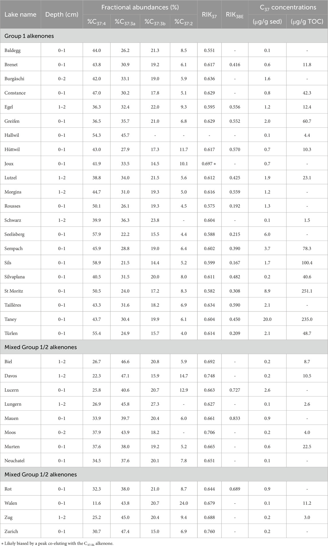
Table 2. C37 alkenone fractional abundances and concentrations together with RIK indices for Swiss lakes containing alkenones. Lakes were separated in two groups, Group 1 and mixed Group 1/2 (see Section 4.1).
All the lakes containing alkenones displayed the tri-unsaturated C37 alkenone isomer (C37:3b) and when alkenones were in sufficient abundance, the alkenone distribution of the lakes featured the complete suite of alkenones including the C38Me, C39Et alkenones and the other tri-unsaturated alkenone isomers (C38:3bEt, C38:3bMe and C39:3b, Figure 2; Table 2). For most lakes, the C37:4 alkenone was the most abundant with C37:4 relative abundances ranging from 36.3% to 58.9% of the total C37 alkenones and an average value of 45.6% (Figure 2A; Table 2; Eq. 3). However, twelve lakes had a C37:3a dominant profile with C37:3a relative abundances ranging from 37.6% to 47.4% of the total C37 alkenones (mean of 42.8%, Figure 2B; Table 2).
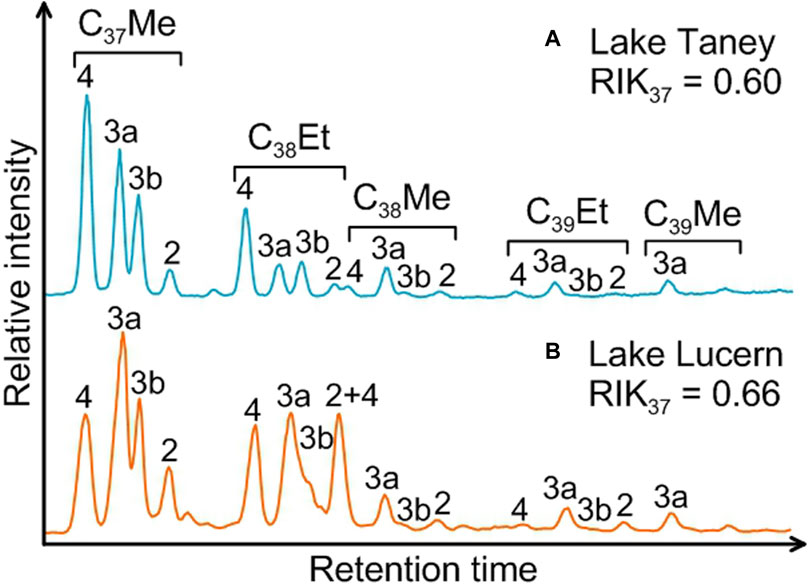
Figure 2. Examples of partial GC-FID chromatograms associated with the RIK37 values for the two typical alkenone distributions found in the studied Swiss lakes: Lake Taney with C37:4 dominant profile (A) and Lake Lucern with C37:3a dominant profile (B).
The RIK37 values (Eq. 4) ranged from 0.55 to 0.76 (mean of 0.64, Figure 3; Table 2) and when it was possible to calculate the RIK38E index (Eq. 5), the values ranged from 0.17 to 0.83 (mean of 0.46, Figure 4; Table 2).
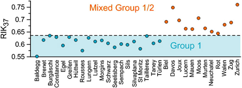
Figure 3. RIK37 values of the studied Swiss lakes. The dashed line represents the upper limit of the RIK37 values for Group 1 Isochrysidales as found by Longo et al. (2018).
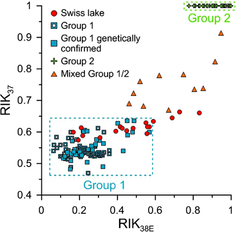
Figure 4. RIK37 and RIK38E values of the studied Swiss lakes (red circle) compared to the ones of Group 2 cultures (green cross), lakes hosting Group 1-type alkenones with (filled blue rectangle) and without genetic confirmation (empty blue rectangle) and mixed Group 1/2 (orange triangle) from the literature. Data are from Longo et al. (2016), Longo et al. (2018), Plancq et al. (2018a, 2019), Richter et al. (2019), Wang et al. (2019), Yao et al. (2019) for Group 1, Longo et al. (2016), Longo et al. (2018), Kaiser et al. (2019), Weiss et al. (2020), Yao et al. (2021), Yao et al. (2022) for mixed Group 1/2 and we used the database of Wang et al. (2022) gathering Group 2 culture data from Nakamura et al. (2014), Araie et al. (2018), Zheng et al. (2019) and Liao et al. (2020).
3.2 Model performance and variable importance
The first random forest model for Swiss lakes (RF1) resulted in an accuracy of 78% (mean accuracy of 76% across the CV folds with a standard error of 12%, Supplementary Table S8), this corresponds to the proportion of test samples correctly classified by the model (Supplementary Text S2). The model was slightly more efficient at correctly classifying lakes with alkenones (sensitivity = 78%, see Supplementary Text S2) than the lakes without alkenones (specificity = 77%, Supplementary Table S8). Reducing the correlations among the variables (RF2) led to very similar results (accuracy of 78%, mean accuracy of 72% ± 3% across the CV folds, Supplementary Table S8). Removing the parameters with negative MDA values slightly improved both model performances (Supplementary Table S8).
The model for the global database and Swiss lakes including all variables (RFG1) resulted in an accuracy of 81% (mean accuracy of 80% ± 2% across the CV folds), a sensitivity of 78% and a specificity of 84%. The performance of the model remained very similar when the correlations among the variables were reduced (RFG2, accuracy of 83%, mean accuracy of 80% ± 3% across the CV folds, Supplementary Table S8).
The indices for variable importance show that Na+ concentration and MAAT are the most important parameters for the Swiss dataset (Figure 5A; Supplementary Figure S3). They are followed by a second group of parameters including conductivity, area, depth and K+ concentration with significantly lower MDA and Gini values. SO42−, O2, total phosphorus and nitrogen (TP and TN) concentrations, stratification, pH and geological catchment have very low values. Depending on the importance index considered (MDA or Gini), Mg2+and Ca2+ concentrations are either in the last or the second group. Lake depth is the most important parameter for the global dataset (Figure 5B; Supplementary Figure S3). MAAT, Na+ and SO42− concentrations come after and then, K+ concentration with elevation. Another group, whose importance index values are lower than 50%, includes Cl− concentration, pH and lake area. Ca2+ concentration and salinity constitute the last group with importance index values lower than 25%. Depending on the importance index considered, Mg2+ concentration is included either in the second or second to last group, while stratification is part of either the second or last group. For both Swiss and global models, the different versions of the models led to very similar importance results (Supplementary Figure S3) highlighting the robustness of the variable importance analysis.
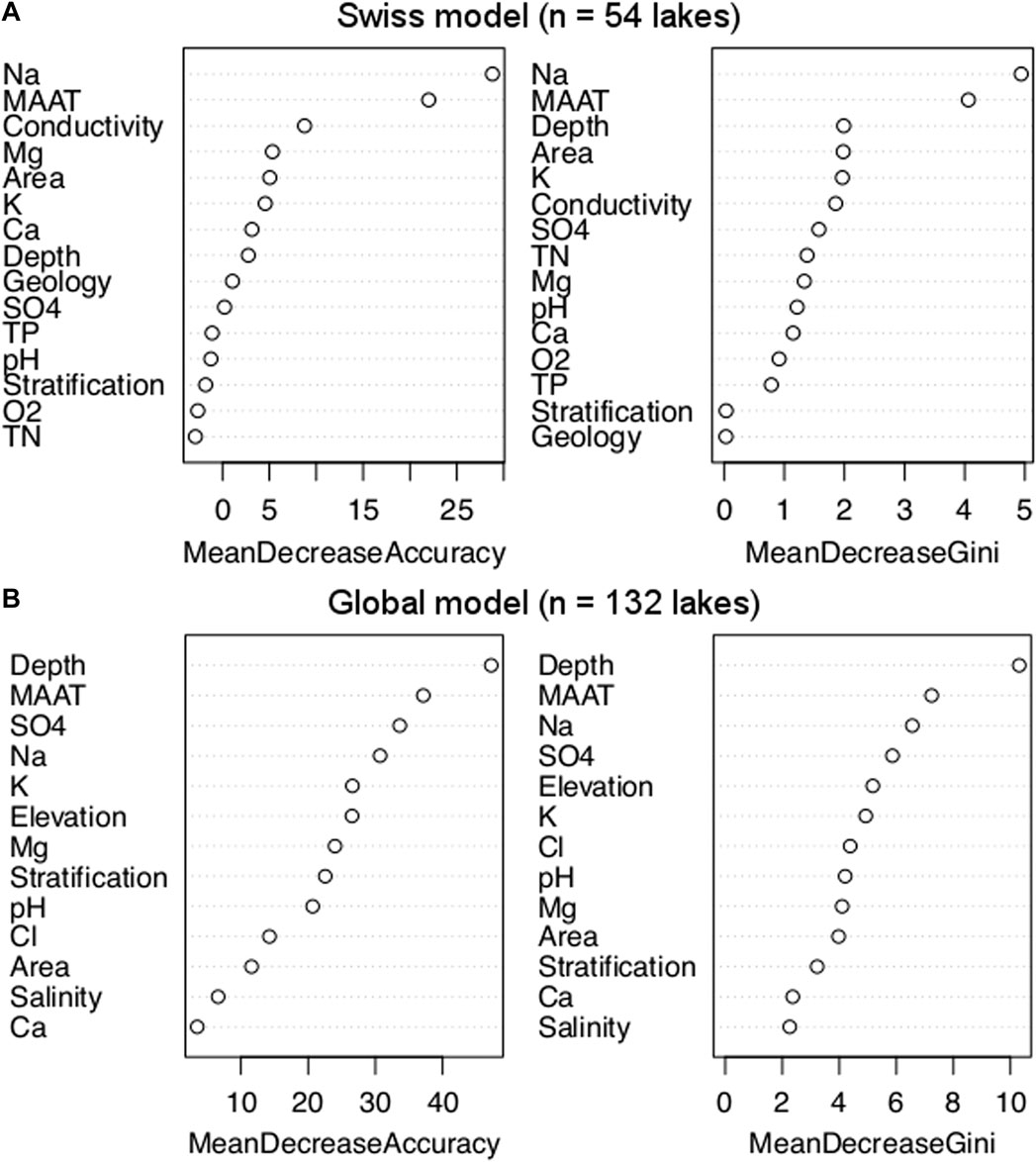
Figure 5. Variable importance measured by mean decrease in accuracy and mean decrease in Gini for the Swiss (A) and global RF models [(B), see Section 2.8.4].
3.3 Probability of alkenone occurrence in freshwater lakes
The ALE plots show the evolution of the probability of alkenone occurrence across the range of values of a given variable. They were compared with the relative frequency distributions of lakes with and without alkenones considering the entire dataset. For almost all variables, both the ALE plots obtained from the Swiss and global models and the distributions of lakes with and without alkenones included one or several optimum(s).
3.3.1 Influence of physical parameters
There are two optimal MAAT ranges for alkenone occurrence: from −17°C to 2°C and between 10°C and 12°C (Figures 6A1–A3). High alkenone concentrations are found within similar temperature ranges (<−3°C, between 0°C and 5°C, and around 10°C, Figure 6A4), most of them being found at MAAT lower than 5°C. The range between 10°C and 12°C is the most favorable for alkenone occurrence but for alkenone abundance, the most favorable range is below 5°C. All the lakes hosting both Group 1 and Group 2 alkenones have MAAT higher than 0°C (except for North Killeak Lake, whose MAAT is −5°C) and most of them are concentrated between 8°C and 12°C (Supplementary Figure S4); whereas most of the lakes containing only Group 1 alkenones have MAAT lower than 6°C, with a peak between −10 and −8°C. We note that in the highest part of the occurrence range of alkenones (12°C–14°C), there are only alkenones whose producers are undetermined (Supplementary Figure S4), making uncertain the upper MAAT limit of Group 1 alkenone occurrence.
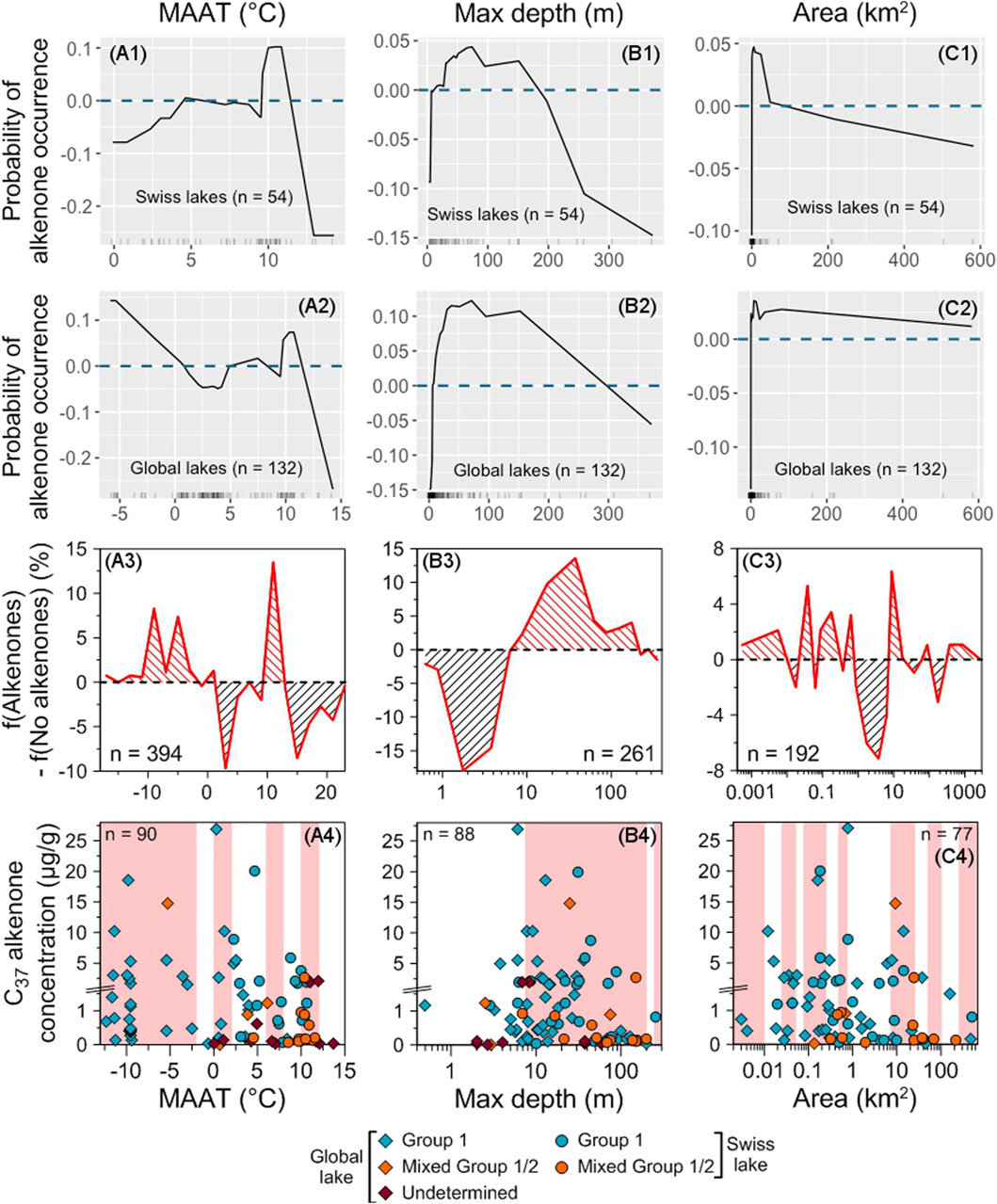
Figure 6. Impact of physical parameters on alkenone occurrence and abundance. Accumulated local effects (ALE) plots for the Swiss (A1–C1) and global (A2–C2) RF models. The dashed blue line represents ALE = 0, indicating that predictions are not significantly affected. The density of feature distribution is shown on the x-axis, with each tick corresponding to one lake. Regions with low density should be interpreted with caution. (A3–C3) Difference between the relative frequencies of Swiss and global lakes with and without alkenones depending on each tested variable. Red (black) hatching indicates favorable (unfavorable) ranges of values for alkenone occurrence (see Section 2.8.6). (A4–C4) Distribution of alkenone concentrations depending on each tested variable. Group 1 alkenones are noted with blue symbols, mixed Group 1/2 with orange ones and alkenones whose group is undetermined with purple ones. Swiss lakes have round symbols while lakes from the global database are noted with diamonds. Red shaded areas highlight the ranges where f(Alkenones) − f(No alkenones) is positive. The total number of lakes where alkenone concentration was measured is indicated. Note that we zoomed in on the concentrations below 1.5 μg/g.
The optimal range for alkenone occurrence is found in lakes with depths ranging from 8 to 200 m (Figures 6B1–B3). The best conditions correspond to lakes with depths ranging from 10 to 50 m, where most of the highest alkenone concentrations are also found (from 6 to 15 m and between 20 and 45 m, Figure 6B4). Mixing of Groups 1 and 2 Isochrysidales are frequent in deep lakes (100–200 m, Supplementary Figure S4), while Group 1 alone are rarer in such lakes.
Stratified lakes are more favorable for alkenone occurrence than mixed lakes (Figures 7A,B). 74% of the mixed lakes in the entire global dataset are devoid of alkenones against 33% of the stratified lakes (Figure 7C). Stratified lakes also host the highest alkenone concentrations and have higher mean alkenone concentrations than mixed lakes (2.8 and 1.6 μg/g sed, respectively, Figure 7D).
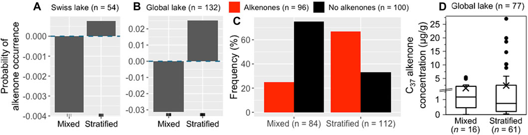
Figure 7. Impact of stratification on alkenone occurrence and abundance. ALE plots for the Swiss (A) and global (B) RF models. The dashed blue line represents ALE = 0, indicating that predictions are not significantly affected. The density of feature distribution is shown on the x-axis, with each tick corresponding to one lake. (C) Histogram showing the relative frequency of stratified and mixed lakes with (red) and without alkenones (black) considering the Swiss and global datasets. (D) Box plot showing the distribution of C37 alkenone concentrations in stratified and mixed lakes from the Swiss and global datasets. The number of lakes where alkenone concentration was measured is indicated for each category. The mean of C37 alkenone concentrations for each category is represented by a black cross. Note that we zoomed in on the concentrations below 1.5 μg/g.
Small (<0.8 km2) and mid-sized lakes (from 8 to 25 km2, Figures 6C1–C3) are favorable for alkenone occurrence. The highest alkenone concentrations are also found in these two ranges (<1 km2 and between 6 and 15 km2, Figure 6C4). Alkenones are more frequent in lakes at low to moderate elevations (Supplementary Figures S2, S5).
3.3.2 Influence of major ions
Ca2+ concentrations lower than 50 mg/L are the most favorable for alkenone occurrence and abundance, even if high concentrations are also favorable, to a lesser extent (Figures 8F1–F4). However, the distribution of the lakes with alkenones depending on Ca2+ concentration is very similar to the one of the lakes without alkenones as well as the one of all studied lakes (Supplementary Figure S2). This suggests that Ca2+ concentration has not much impact on alkenone occurrence as also indicated by the global model (Figure 5B, Supplementary Figure S3).
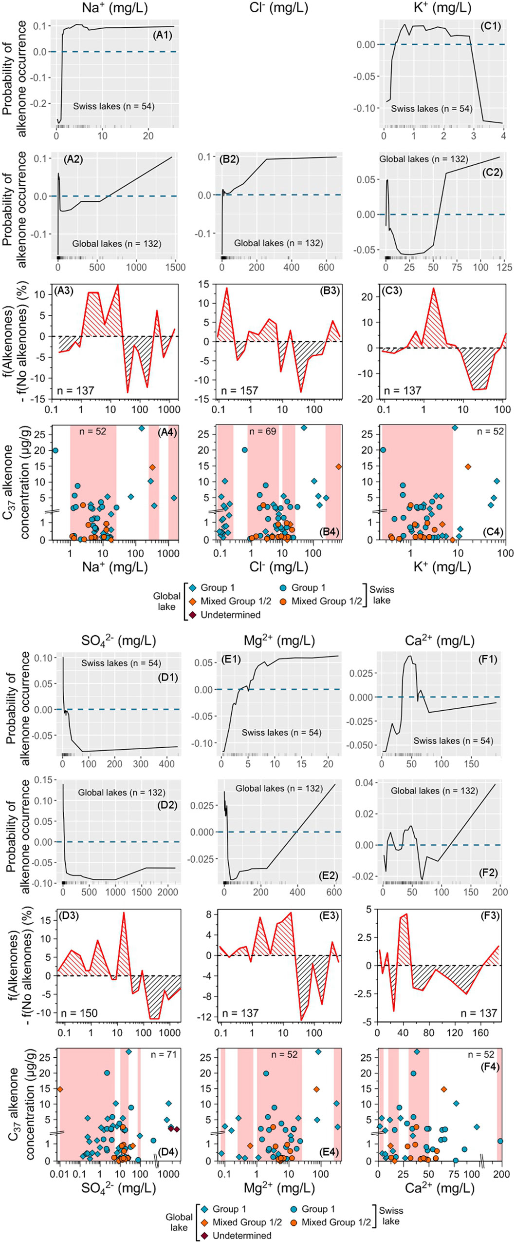
Figure 8. Impact of major ion concentrations on alkenone occurrence and abundance. ALE plots for the Swiss (A1–F1) and global (A2–F2) RF models. The dashed blue line represents ALE = 0, indicating that predictions are not significantly affected. The density of feature distribution is shown on the x-axis, with each tick corresponding to one lake. Regions with low density should be interpreted with caution. Cl− concentration was excluded from the Swiss model (see Section 2.8.2) so, there is no ALE plot for this ion for the Swiss model. (A3–F3) Difference between the relative frequencies of Swiss and global lakes with and without alkenones depending on each tested variable. Red (black) hatching indicates favorable (unfavorable) ranges of values for alkenone occurrence (see Section 2.8.6). (A4–F4) Distribution of alkenone concentrations depending on each tested variable. Group 1 alkenones are noted with blue symbols, mixed Group 1/2 with orange ones and alkenones whose group is undetermined with purple ones. Swiss lakes have round symbols while lakes from the global database are noted with diamonds. Red shaded areas highlight the ranges where f(Alkenones) − f(No alkenones) is positive. The total number of lakes where alkenone concentration was measured is indicated. Note that we zoomed in on the concentrations below 1.5 μg/g.
For the remaining considered ions, the optimal range for alkenone occurrence is found at low concentrations: between 0.3 and 8 mg/L for K+ and lower than 25 mg/L for the other ions (Figures 8A1–E3). Most of the highest alkenone concentrations are included in these ranges and are generally divided into two peaks: one at very low ion concentrations (<∼ 2 mg/L) and another in the high part of the range (between 2 and 4.5 mg/L for K+ and between ∼7 and 20 mg/L for the other ions, Figures 8A4–E4). It seems that there is a threshold for alkenone occurrence corresponding to a Na+ concentration close to 1 mg/L. It is not a strict threshold though, as alkenones are present in Lake Taney (Switzerland), which has a Na+ concentration of 0.4 mg/L and hosts the second highest alkenone concentration of the database (Supplementary Tables S1, S3).
However, for all ions, there is a second minor favorable range for alkenone occurrence at higher concentrations (Figures 8A2–E2). This range is found for ion concentrations higher than 250 mg/L for Na+ (250–500 mg/L and 1,000–2,000 mg/L), Cl− (250–750 mg/L) and Mg2+ (250–500 mg/L), between 100 and 140 mg/L for K+ and between 75 and 100 mg/L for SO42− (Figures 8A3–E3). A small group of lakes with high ion concentrations contain high alkenone concentrations, including Lake Matarak, which hosts the highest alkenone concentration of the database (Figures 8A4–E4; Supplementary Table S3). Among these lakes, North Killeak Lake in Alaska, contains Group 2 Isochrysidales in very small quantities together with Group 1 and has the highest Cl− concentration of the global database as well as the lowest SO42− concentration, which are both outside of the range for lakes containing only Group 1 (Figures 8B4, D4; Supplementary Table S3; Supplementary Figure S4). Two lakes containing alkenones whose group is unknown also have the highest SO42- concentrations of the global database (Figure 8D4; Supplementary Table S3; Supplementary Figure S4), but lakes containing Group 1 alkenones have close SO42− concentrations.
Apart from North Killeak Lake, the lakes hosting both Group 1 and Group 2 Isochrysidales have a distribution similar to the one of the lakes containing only Group 1; even if their occurrence range is often narrower, which is likely due to their smaller number. In particular, the mixing of both groups is not found at Cl− concentrations lower than 1 mg/L, while almost one-third of the lakes hosting the Group 1 alone are found below this value (Supplementary Figure S4). The situation is similar for SO42− concentrations, where lakes with mixed Group 1/2 are mainly concentrated in the range 10–50 mg/L, while lakes with Group 1 are more widely distributed (Supplementary Figure S4).
3.3.3 Influence of salinity, conductivity, alkalinity and pH
In freshwater lakes, low salinities appear as the most favorable for alkenone occurrence (<0.1 and between 0.2 and 0.6 g/L, Figures 9A1–A3). The highest concentrations are also found at low salinities (<0.6 g/L) but there is another peak of high alkenone concentrations between 1 and 1.5 g/L (Figure 9A4).
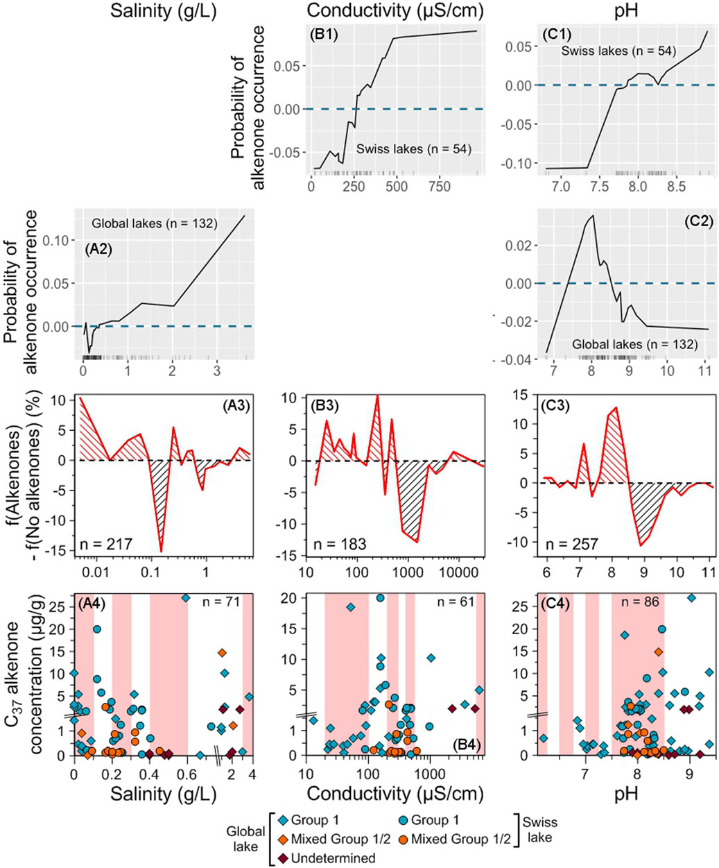
Figure 9. Impact of salinity, conductivity and pH on alkenone occurrence and abundance. ALE plots for the Swiss (B1–C1) and global (A2,C2) RF models. The dashed blue line represents ALE = 0, indicating that predictions are not significantly affected. The density of feature distribution is shown on the x-axis, with each tick corresponding to one lake. Regions with low density should be interpreted with caution. Salinity was excluded from the Swiss model and conductivity from the global model (see Section 2.8.2) so, there is no ALE plots for these variables for the Swiss model and the global model, respectively. (A3–C3) Difference between the relative frequencies of Swiss and global lakes with and without alkenones depending on each tested variable. Red (black) hatching indicates favorable (unfavorable) ranges of values for alkenone occurrence (see Section 2.8.6). (A4–C4) Distribution of alkenone concentrations depending on each tested variable. Group 1 alkenones are noted with blue symbols, mixed Group 1/2 with orange ones and alkenones whose group is undetermined with purple ones. Swiss lakes have round symbols while lakes from the global database are noted with diamonds. Red shaded areas highlight the ranges where f(Alkenones) − f(No alkenones) is positive. The total number of lakes where alkenone concentration was measured is indicated. Note that we zoomed in on the concentrations below 1.5 μg/g.
Low (from 20 to 100 μS/cm) and moderate conductivity values (between 200 and 300 μS/cm and 400–550 μS/cm) are favorable for alkenone occurrence, the range 200–300 μS/cm being the most favorable (Figures 9B1–B3). The highest alkenone concentrations are also found at moderate conductivity values (between 80 and 265 μS/cm, Figure 9B4). At conductivities higher than 550 μS/cm, the conditions are not favorable for alkenone occurrence except between 5,500 and 10,000 μS/cm (Figure 9B3). A small group of lakes with high alkenone concentrations are found at high conductivity (>1,000 μS/cm, Figure 9B4).
As found for conductivity, low to moderate alkalinity values (from 1 to 100 mg/L) are the most favorable for alkenone occurrence and abundance (Figure 10). The distribution of lakes with mixed Group 1/2 alkenones is different from the one of Group 1 alone but this is mainly due to the reduced number of data for lakes with mixed Group 1/2 (Supplementary Figure S4).
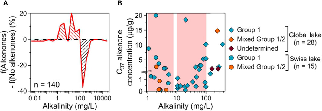
Figure 10. Impact of alkalinity on alkenone occurrence and abundance. (A) Difference between the relative frequencies of Swiss and global lakes with and without alkenones depending on alkalinity. Red (black) hatching indicates favorable (unfavorable) ranges of values for alkenone occurrence (see Section 2.8.6). (B) Distribution of alkenone concentrations depending on alkalinity. Group 1 alkenones are noted with blue symbols, mixed Group 1/2 with orange ones and alkenones whose group is undetermined with purple ones. Swiss lakes have round symbols while lakes from the global database are noted with diamonds. Red shaded areas highlight the ranges where f(Alkenones) − f(No alkenones) is positive. Note that we zoomed in on the concentrations below 1.5 μg/g.
The most favorable conditions for alkenone occurrence are found for pH ranging from 7.0 to 8.5, especially from 7.5 to 8.5 (Figures 9C1–C3). Most of the highest alkenone concentrations are also found in this range (Figure 9C4).
3.3.4 Influence of nutrients and trace elements
Low concentrations of TN, TP (<1.5 and <0.1 mg/L, respectively, Figures 11A–D) and trace elements (Supplementary Figure S6) are the most favorable for alkenone occurrence. The highest alkenone concentrations are also found at low TN, TP (<0.1 mg/L for TP and <1 mg/L for TN, Figures 11E,F) and trace element concentrations (Supplementary Figure S7).
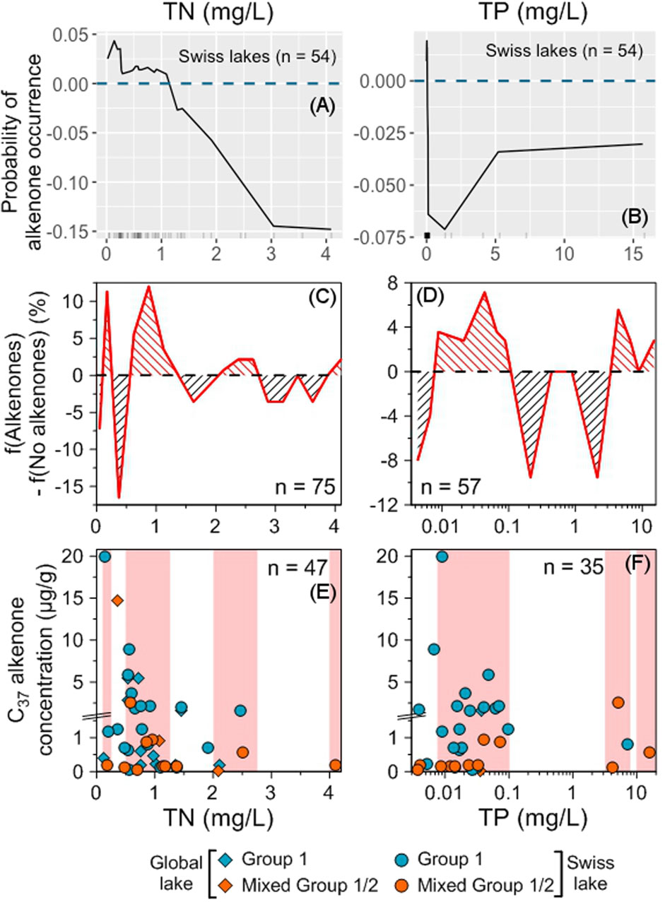
Figure 11. Impact of nutrient concentrations on alkenone occurrence and abundance. ALE plots for the Swiss RF model (A,B). The dashed blue line represents ALE = 0, indicating that predictions are not significantly affected. The density of feature distribution is shown on the x-axis, with each tick corresponding to one lake. Regions with low density should be interpreted with caution. Difference between the relative frequencies of Swiss and global lakes with and without alkenones depending on each tested variable (C,D). Red (black) hatching indicates favorable (unfavorable) ranges of values for alkenone occurrence (see Section 2.8.6). Distribution of alkenone concentrations depending on each tested variable (E,F). Group 1 alkenones are noted with blue symbols and mixed Group 1/2 with orange ones. Swiss lakes have round symbols while lakes from the global database are noted with diamonds. Red shaded areas highlight the ranges where f(Alkenones) − f(No alkenones) is positive. The total number of lakes where alkenone concentration was measured is indicated. Note that we zoomed in on the concentrations below 1.5 μg/g.
Increasing probabilities of alkenone presence were associated with cold or mild temperatures, small to mid-sized stratified freshwater lakes with depths ranging from 10 to 50 m, low ion concentrations, low salinities, low to moderate conductivity and alkalinity values, moderately alkaline pH (7.0–8.5) and low nutrient and trace element content. These favorable conditions for alkenone presence generally coincide with the ranges where alkenones are present in high concentrations in our global dataset of freshwater lakes.
4 Discussion
4.1 Alkenone distributions and diversity in Swiss lakes
Alkenones were detected in 59% of the studied lakes (Figure 1A; Table 1). The concentrations of C37 alkenones in Swiss lakes (from 0.1 to 20.0 μg/g, mean 1.9 μg/g, Table 2) are similar to those of the global database (from 0.01 to 27.0 μg/g, mean of 2.5 μg/g, Supplementary Table S3). The highest alkenone concentrations were reported in Greenland Lake BrayaSø (82.7 mg/g TOC, D’Andrea and Huang, 2005).
The tri-unsaturated C37 alkenone isomer (C37:3b), which is specific to the Group 1 Isochrysidales (Longo et al., 2016) is present in all the Swiss lakes containing alkenones, as well as the complete suite of alkenones including the C38Me, C39Et alkenones and the other tri-unsaturated alkenone isomers (C38:3bEt, C38:3bMe and C39:3b), when alkenones were in sufficient abundance (Figure 2; Table 2). Most lakes had distributions dominated by the C37:4 alkenone (36.3%–58.9% of the total C37 alkenones, mean of 45.6%, Figure 2A; Table 2), which are characteristic of Group 1-type alkenones.
Longo et al. (2016) defined the isomeric ratio of ketones RIK37 (Eq. 4) based on the specificity of the C37:3b isomer to the Group 1 Isochrysidales to differentiate the Group 1 alkenone distributions from Group 2 and Group 3 distributions. The majority of our lakes (20 lakes) had RIK37 values ranging from 0.55 to 0.64 (mean of 0.61, Figure 3; Table 2). This falls within the RIK37 range (0.48–0.64) defined by Longo et al. (2018) for freshwater lakes in the Northern Hemisphere containing Group 1-type alkenones (Supplementary Table S10). RIK37 values of 1, in contrast, indicate that the alkenones are only produced by Group 2 or Group 3 Isochrysidales.
Twelve lakes had a C37:3a dominant profile (37.6%–47.4% of the total C37 alkenones, mean of 42.8%, Figure 2B; Table 2). These 12 lakes had RIK37 values higher than 0.64 (0.64–0.76 with a mean value of 0.68) except for Lake Lungern, which had a RIK37 value of 0.63 (Figure 3; Table 2). This suggests that these 12 lakes likely contain both Group 1 and Group 2 Isochrysidales. Lake Joux had a RIK37 value higher than 0.64 (0.70), even though it had a distribution characteristic of Group 1 Isochrysidales with a dominant C37:4 peak (Figure 3; Table 2). However, another compound co-eluted with the C37:3b alkenone, which persisted even after saponification and silver-nitrate purification, and likely biased the RIK37 value.
The C38:3bEt isomer can also be used to separate alkenone distributions by phylotype through the isomeric ratio of ketones RIK38E defined by Longo et al. (2016) (Eq. 5). Unfortunately, we were not able to calculate the RIK38E values for all the samples due to low abundances or the presence of co-eluting compounds. However, in Swiss lakes where we were able to calculate the RIK38E index, the values were lower than 0.57 (0.17–0.57, mean value of 0.39) except in Lakes Taillères, Rot, Lucern and Mauen (RIK38E values of 0.59, 0.69, 0.73 and 0.83, respectively, Figure 4; Table 2). The C38:3bEt isomer is produced by some Group 2 Isochrysidales in trace amounts, therefore RIK38E values ranging from 0.75 to 1 are inferred as containing Group 2 Isochrysidales while values between 0 and 0.57 likely reflect Group 1-type alkenones in Northern Hemisphere lakes (Supplementary Table S10; Longo et al., 2016; Longo et al., 2018). Based on the RIK38E index, the majority of our lakes likely contain Group 1 alkenones.
Combining RIK37 and RIK38E values for Group 1 and Group 2 Isochrysidales from the literature with our data allows us to confidently infer, in agreement with our previous conclusions, that the majority of Swiss lakes likely contain only Group 1 Isochrysidales (Figure 4). Lakes Rot, Lucern and Mauen are outside of the Group 1 range (Figure 4), as well as the eight other lakes with RIK37 values higher than 0.64 (Figure 3; Table 2). The higher RIK37 values are consistent with lakes that host a mix of Group 1 and Group 2 Isochrysidales (Figure 4; Supplementary Table S10). The RIK37 and RIK38E values of these 11 lakes remain closer to the Group 1 haptophyte upper limits than the Group 2 Isochrysidales lower limits, suggesting that Group 1 Isochrysidales may be more abundant in these lakes than Group 2 Isochrysidales.
Lake Taillères stands at the limits of the Group 1 range (Figure 4), as well as Lake Burgäschi (Figure 3). The RIK37 values of these two lakes (0.63 and 0.64, respectively, Table 2) are less than or equal to the upper limit of the RIK37 values of lakes hosting genetically confirmed Group 1 Isochrysidales (0.64, Supplementary Table S10), which was recorded in Lake Schmaler Luzin in Germany (Longo et al., 2018). Thus, these two lakes are included in the Group 1 range. However, the RIK38E value of Lake Taillères slightly exceeds the known range of RIK38E values for Group 1 Isochrysidales (0.59 versus 0.57, Table 2; Supplementary Table S10), suggesting that the range of RIK38E values for Group 1 Isochrysidales should be extended. Yao et al. (2019) pointed out that the primers used in many of the marker gene analyses would not pick up Group 1 Isochrysidales belonging to the Group 1b (formerly EV clade). Thus, the true range of lakes harboring Group 1 Isochrysidales is not fully considered. The alternative is that Lake Taillères hosts a small proportion of Group 2 Isochrysidales.
The twelve lakes likely containing a mix of Group 1 and 2 Isochrysidales have a higher proportion of C37:3a than C37:4 (mean of 42.8% vs. 28.8%, Figure 2B; Table 2). Previous studies, identified three subclades within Group 2 that correspond to different ecological niches within saline lakes: Group 2i and 2w1 that mainly occur at low and intermediate salinities; and Group 2w2 that prefers to occur in hypersaline lakes (Wang et al., 2021; Yao et al., 2022). The mixed alkenone profiles found in the Swiss lakes, likely correspond to Group 1 and 2w1 Isochrysidales. Typical chromatograms of dominant Group 2w1 contain a higher proportion of C37:3a compared to the C37:4 alkenone; unlike Group 2i, which is characterized by a high C37:4 proportion (Yao et al., 2022). Moreover, the characteristic alkenone of Group 2i, the C39:4Me alkenone, is absent from our chromatograms (Yao et al., 2022; Figure 2B). One likely scenario is that the ice-associated Isochrysidales are represented by Group 1’s in these lakes - often detected during ice-off. The presence of Group 2w2 seems unlikely as these alkenone producers prefer hypersaline lakes (Yao et al., 2022). Moreover, Swiss lakes correspond to the known ecological preferences of Group 2w1 Isochrysidales: they have low salinities and low abundances of Na+ and Cl− (Supplementary Table S1) (Yao et al., 2022).
Group 2 Isochrysidales are mainly found in oligohaline to hyperhaline lakes (e.g., Longo et al., 2016; Yao et al., 2020; 2022). The transition from Group 1 to Group 2 Isochrysidales has been found to occur across a salinity range of ∼1–10 g/L (Yao et al., 2020). However, here we report Group 2 alkenones in 12 lakes with salinities lower than 0.45 g/L (Table 1). Yao et al. (2019) and Wang et al. (2019) also detected Group 2 Isochrysidales, in small number, in freshwater lakes from China and Alaska based on genomic analyses; while Yao et al. (2021) found Group 2 Isochrysidales together with Group 1 in 5 Chinese lakes with salinity ranging from 0.7 to 2.07 g/L. Therefore, Group 2 Isochrysidales seem to be more common than initially thought in lakes with low salinities.
In conclusion, all the studied lakes in Switzerland containing alkenones have a characteristic Group 1 signature. The alkenone distributions of 12 lakes indicate that they likely contain both Group 1 and Group 2, more specifically Group 2w1 Isochrysidales, with the Group 1 being present in higher abundance. Marker gene analyses will be conducted in the future to further explore the composition of the Isochrysidales communities in Swiss lakes. Alkenones were also found in freshwater lakes in the United Kingdom, Germany, and France (Cranwell, 1985; Zink et al., 2001; Simon et al., 2013; 2015; Figure 1B), suggesting that alkenones are common in mid-latitude European freshwater lakes.
4.2 Parameters influencing alkenone occurrence and abundance in freshwater lakes
4.2.1 Variable importance
Both Swiss and global models found Na+ concentration and MAAT among the most important variables for alkenone occurrence (Figure 5; Supplementary Figure S3). Depth appears less important in the Swiss model compared to the global model, where it is the most important variable (Figure 5; Supplementary Figure S3). These results are consistent with those of the model of Plancq et al. (2018a): where water temperature and depth were among the most important parameters influencing alkenone occurrence, while stratification and pH appeared less important (Figure 5B; Supplementary Figure S3). However, Plancq et al. (2018a) found salinity to be the main variable determining alkenone occurrence, whereas it is one of the least important parameters in our global RF model (Figure 5B; Supplementary Figure S3); although salinity is highly correlated with Na+ and SO42− concentrations (r = 0.88 and 0.86, respectively, Supplementary Table S9), which rank among the most important parameters.
Na+ is a dominant cation in 45% of the lakes for which major ion compositions are available in the entire global dataset (n = 168, Supplementary Tables S1, S3) but Ca2+ is dominant in 52% of them, Mg2+ in 14% and K+ in 1%. The proportions are similar in the lakes used for the global model (44% for Na+, 58% for Ca2+, 11% for Mg2+ and 1% for K+, Supplementary Table S6). In fact, salinity is more correlated with the sum of the cations than with Na+ alone (R2 = 0.89 and 0.77, respectively, Supplementary Figure S8). Therefore, in freshwater lakes, salinity is also influenced by other ions which are less important for alkenone occurrence than Na+ or SO42- such as Ca2+ and Cl− (Figure 5; Supplementary Figure S3). This could explain the low importance of salinity in our model. On the other hand, Na+ is the main ion responsible for salinity in saline lakes. In the study of Plancq et al. (2018a), which includes mainly saline lakes, with salinity ranging from 0.1 to 102 g/L, Na+ is by far the most correlated ion with salinity (R2 = 0.90 against 0.55 for HCO3−, the second highest correlated ion). Therefore, it seems likely that Group 1 (dominant in freshwater lakes) and Group 2 alkenones (dominant in saline lakes) occurrence are mainly controlled by the same parameters: Na+ concentration, depth and temperature.
In the Swiss dataset, Na+ and Cl− concentrations are highly correlated (r = 0.93, Supplementary Table S7). This likely reflects a common source for both ions in Swiss lakes, probably halite. Both ions are often increased by anthropogenic sources (e.g., Müller and Gächter, 2012). However, they are less correlated in the global model (r = 0.53, Supplementary Table S9) whose results suggest that Cl− concentration has a limited importance for alkenone occurrence (Figure 5B; Supplementary Figure S3). More generally, ions are intercorrelated in both datasets: K+ and Na+ are linked within the Swiss dataset as well as SO42− and Ca2+ (r = 0.76 in both cases, Supplementary Table S7), while in the global dataset, SO42− is strongly correlated with Mg2+ and Na+ (r = 0.87 and 0.77, respectively), and Mg2+ with K+ (r = 0.75, Supplementary Table S9).
4.2.2 Impact on the probability of alkenone occurrence and potential biological mechanisms
For almost all variables, the range of values for Swiss lakes is significantly narrower than the one of the lakes of the global model (Supplementary Tables S1, S6). Yet, in most cases, the trends of the probability of alkenone occurrence for a given variable obtained from the Swiss and the global models were similar or compatible (Figures 6A1–C2, 7A,B, 8A1–F2, 9C1–C2). The results of the ALE plots are also, in most cases, in agreement with the distribution of the lakes with and without alkenones in the entire global dataset, even when the number of samples is significantly higher than in the models (Figures 6A1–C3, 7A–C, 8A1–F3, 9B1–C3, 11A–D). This suggests that the environmental parameters controlling the occurrence of alkenone producers in freshwater lakes are similar across regions. However, in most cases, we note some lakes containing alkenones outside of the most favorable ranges (Supplementary Figure S2), which reveals an important flexibility of alkenone producers in freshwater lakes, allowing them to adapt to a variety of environmental conditions.
4.2.2.1 Impact of physical parameters
Regarding physical parameters, alkenones are most probably found in small to mid-sized stratified freshwater lakes with depths ranging from 10 to 50 m, in cold or mild environments (MAAT <2°C or between 10°C and 12°C, Figures 6, 7). These are also the best conditions for finding high alkenone concentrations, except for MAAT for which the best conditions are found in colder environments (<5°C, Figures 6, 7).
Studies of modern lakes have reported alkenones in freshwater lakes primarily located in the mid and high latitudes of the Northern Hemisphere where MAAT ranges from −17.3°C to 13.7°C (Figure 1B; Supplementary Figure S2; Supplementary Table S3). As highlighted by Brassell et al. (2022), there are very few lakes where the presence or absence of alkenones has been reported in the tropics and the Southern hemisphere, which potentially biases the extent of occurrence of global lacustrine alkenones.
Several studies previously noted that cold environments were more favorable for alkenone occurrence and abundance (Cranwell, 1985; Zink et al., 2001; Chu et al., 2005; Plancq et al., 2018a; Longo et al., 2018). Plancq et al. (2018a) found the highest probability for alkenone occurrence in the coldest Canadian lakes. Cranwell (1985) and Zink et al. (2001) also reported high alkenone concentrations in sediment records from cold time periods, when alkenones were absent or present in low abundance in modern surface sediments that are considerably warmer. Higher alkenone concentrations were also observed under colder marine temperatures (Sikes et al., 1997; Volkman et al., 1998). Zink et al. (2001) proposed that alkenone producers, unlike other common lacustrine algal species, are resistant to low temperatures and encounter less competition in cold environments. Our results support these previous conclusions, that alkenone producers are more common and abundant in low temperature settings (Figures 6A1–A4).
MAAT appears as one of the most important parameters in the models (Figure 5; Supplementary Figure S3). Indeed, temperature in general is one of the driving factors in controlling microbial diversity and distributions in nature and one of the most important factors driving growth of primary producers (e.g., Eppley, 1971). Temperature impacts many aspects of algal physiology - the most prominent includes chemical reactions and transport processes (Raven and Geider, 1988). In the case of Isochrysidales, temperatures certainly play a role in the expression of desaturases that are used to catalyze the alkenone desaturation reaction that is upregulated during cold stress (Endo et al., 2018).
Depth was already proposed as an important parameter for alkenone occurrence and abundance: alkenones are more frequent and abundant in deeper lakes (Toney et al., 2010; Longo et al., 2016; Plancq et al., 2018a). However, these previous studies only looked at lakes with a narrow range of depth (0–30 m). Extending the range of depth reveals that after reaching a peak in lakes with depths between 10 and 50 m, the proportion of lakes with alkenones and their concentrations decrease (Figures 6B1–B4).
Depth is the most important parameter in the global model (Figure 5B; Supplementary Figure S3); while it appears less important in the Swiss model (Figure 5A; Supplementary Figure S3). The Swiss and the global datasets have similar depth ranges (2.9–372 m and 0.5–197 m, respectively, Table 1; Supplementary Table S3). However, lakes with depth shallower than 10 m were under-sampled in the Swiss dataset compared to the global dataset (Supplementary Figure S9). These shallow lakes appear to be very unfavorable for alkenone occurrence (Figure 6B3) but this is not visible in the Swiss dataset as they are under-represented. Moreover, mid-sized Swiss lakes appear only slightly favorable for alkenone occurrence (Supplementary Figure S9); this likely means that even if water depth could be an important parameter, as suggested by the global model (Figure 5B; Supplementary Figure S3), other parameters also influence alkenone occurrence in Swiss lakes.
Depth could influence Isochrysidales life cycle. Indeed, the bloom of Group 1 and some Group 2 Isochrysidales is thought to be influenced by the increase of light penetration during and after ice-off (Toney et al., 2010; D’Andrea et al., 2011; Ellegaard et al., 2016). A moderate lake depth would be advantageous to detect and respond to the light changes. The life cycle of some alkenone producers is thought to include a benthic vegetative stage (Toney et al., 2010; Ellegaard et al., 2016; Theroux et al., 2020) but we do not know if this is true of all. Deeper lake depth favors stratification, which is thought to favor alkenone producers by offering a physical “refuge” for the resting cells (Toney et al., 2010; 2011; Plancq et al., 2018a). Stratified lakes are indeed more favorable for alkenone presence and abundance than mixed lakes (Figure 7). Toney et al. (2010) and Plancq et al. (2018a) also found the highest alkenone concentrations in stratified lakes, especially lakes with permanent stratification and deep-water anoxia. However, in the Swiss model, stratification appears as one of the least important parameters (Figure 5A; Supplementary Figure S3). This may be due to the low number of mixed lakes in the Swiss dataset (9 lakes out of 54, Table 1). In the global model, the relative MDA value for stratification is 50%, which suggests that its influence on alkenone occurrence is limited (Figure 5B; Supplementary Figure S3). Yet, spring mixing seems to influence the bloom timing of Group 1 Isochrysidales (e.g., Longo et al., 2016; 2018; Richter et al., 2019) as well as some Group 2 Isochrysidales (e.g., Toney et al., 2010; Theroux et al., 2020). Therefore, mixing regime could play an important role in the life cycle of alkenone producers in freshwater lakes. This data is often missing in previous studies and more data would be necessary to test if dimictic lakes are more favorable than other types of lakes.
Lake area was never considered as a parameter that could influence alkenone occurrence. The distribution of the lakes with alkenones depending on lake area is very similar to the one of the lakes without alkenones as well as the one of all studied lakes (Supplementary Figure S2). This suggests that area does not have a strong influence on alkenone occurrence, which is also indicated by the global model (Figure 5B; Supplementary Figure S3).
Elevation appears as an important parameter in the global model (Figure 5B; Supplementary Figure S3). However, elevation is not expected to directly impact alkenone producers. Elevation does not show any strong correlation in the global model (Supplementary Table S9) but it is likely correlated with stratification. The pattern of alkenone occurrence more likely reflects the distribution of the studied lakes rather than a biological influence of elevation on alkenone producers.
4.2.2.2 Impact of major ions
Only a few studies reported major ion concentrations in connection with alkenones, thus the impact of major ion concentrations on the occurrence of alkenones has rarely been assessed.
On one hand, Yao et al. (2019) suggested that high major ion concentrations, especially Na+, K+ and Mg2+, were unfavorable for Group 1 alkenones and Toney et al. (2011) suggested as well that high Mg2+ concentrations could be unfavorable for alkenone producers. On the other hand, Toney et al. (2010) and Toney et al. (2011) found that alkenones were present in high abundances in lakes with high Na+ and K+ concentrations and suggested that elevated Na+ concentration may be critical for alkenone occurrence. Our results showing two optimal ranges for alkenone occurrence and abundance, one at low ion concentration and a minor one at high concentrations (Figure 8), reconcile previous studies that only detected one of these optima due to reduced range of study. Elevated SO42- concentrations were suggested to favor alkenone presence and abundance in freshwater and saline lakes (Pearson et al., 2008; Toney et al., 2010; 2011; Zhao et al., 2014; Longo et al., 2016). However, considering only freshwater lakes, low SO42- concentrations appear to be the most favorable conditions (Figures 8D1–D4).
SO42-, K+, Ca2+ and Mg2+ are essential for green plants, where they play a role in various critical functions such as activation of enzymatic reactions, maintenance of membrane potential and osmotic homeostasis, as well as negative and positive charge equilibrium, and redox buffer (Maathuis, 2009). Unicellular phototrophs require similar mineral macronutrients to complete their life cycle, despite being evolutionarily distantly related (Bhattacharya and Medlin, 1998). However, when present in high quantities, some ions can have negative effects; high SO42- concentrations can be toxic (Maathuis, 2009) and elevated Na+ concentrations alter the osmotic regulation, protein synthesis and photosynthesis, in particular through over-competition with other cations (EL-Sheekh, 2004; Singh et al., 2018). Several experiments observed a decrease of algal growth with increasing input of NaCl (Gorain et al., 2013; Battah et al., 2014; Sikorski, 2021). Na+ is often abundant in the environment thus, organisms have to maintain a low level of Na+ in their cells (Li et al., 2023). Isochrysidales seem to be well adapted to do so given that there have been multiple marine-freshwater transitions in the evolution of haptophytes (Simon et al., 2013). K+ can help algae deal with salt and alkali stress (Li et al., 2023). In fact, organisms maintain a high level of K+ in their cells, while this ion is usually present in low concentrations in the environment, and some K+ transport systems were found to help algae maintain the high K+/Na+ ratio, making them tolerant to high Na+ and low K+ conditions (Li et al., 2023). However, in freshwater lakes, Isochrysidales seem to prefer lakes with low Na+ concentrations, even if they can live in lakes with higher concentrations (Figure 8A3; Supplementary Figure S2). The lipid content of algae was found to increase with NaCl input (Rao Ranga et al., 2007; Gorain et al., 2013; Singh et al., 2018). A similar mechanism could explain the higher alkenone concentrations found in saline lakes as a response to saline stress (see Section 4.2.2.3). A lack of Ca2+ also resulted in a rise in lipid content, while an increase of Mg2+ led to the same result and was accompanied by an increase in biomass (Gorain et al., 2013). Accordingly, all these ions appear as relatively important for alkenone occurrence in the models, except Cl− and Ca2+, which is maybe more important for plants than for algae (Figure 5; Supplementary Figure S3).
4.2.2.3 Impact of salinity, conductivity, alkalinity and pH
Freshwater lakes with low salinity, low to moderate conductivity and alkalinity values and moderately alkaline pH (7.0–8.5) are the most favorable for alkenone occurrence (Figures 9, 10). The ranges for high alkenone concentrations are similar for conductivity and alkalinity but different for salinity (<0.6 g/L and between 1 and 1.5 g/L) and pH (7.7–9.4, Figures 9, 10).
Salinity was identified as an important control on alkenone presence in lakes (D’Andrea and Huang, 2005; Pearson et al., 2008; Toney et al., 2010; 2011; Song et al., 2016; Plancq et al., 2018a; Bulkhin et al., 2023). Indeed, alkenones are more frequently reported and present in higher concentrations in saline lakes compared to freshwater lakes (e.g., Chu et al., 2005; Toney et al., 2010; Song et al., 2016; Plancq et al., 2018a; Bulkhin et al., 2023). However, several studies already demonstrated that elevated salinity is not a strict requirement for the occurrence of alkenones (e.g., Cranwell, 1985; Zink et al., 2001; Longo et al., 2016; Longo et al., 2018; McColl, 2016).
Considering only freshwater lakes (maximal salinity of 3 g/L except for two exceptions at 3.6 and 7.1 g/L, see Section 2.3), low salinities appear as the most favorable for alkenone occurrence (<0.1 and between 0.2 and 0.6 g/L, Figures 9A1–A3) and abundance (<0.6 g/L) Figures 9A4. Mixing of Groups 1 and 2 alkenones are slightly more frequent in lakes with higher salinities (>0.7 g/L, Supplementary Figure S4) compared to Group 1 alone. Wang et al. (2019) suggested that the presence of Group 2 Isochrysidales in North Killeak Lake could be linked to the relatively high salinity of the lake (1.1 g/L, Supplementary Table S3). However, the mixing occurs at salinity as low as 0.04 g/L (Supplementary Table S3) and most lakes with mixed Group 1/2 are found between 0.1 and 0.5 g/L (Supplementary Figure S4). Salinity plays a role in shaping microbial communities but it is mainly linked with NaCl whose effects were discussed above.
The influence of conductivity on alkenone presence was already reported; D’Andrea and Huang (2005) and Longo et al. (2016) noted that lakes with elevated conductivity are favorable for alkenone occurrence and abundance. Elevated alkalinity values were also reported to be favorable for alkenone occurrence and abundance in previous studies (Longo et al., 2016; Wang et al., 2019). However, Zink et al. (2001) noted that high alkalinity was not mandatory for alkenone occurrence. Extending the number of lakes and the range of conductivity and alkalinity values demonstrates that lakes with low to moderate conductivity and alkalinity values are the most favorable for alkenones (Figures 9B1–B4, 10).
The optimal range for alkenone occurrence and abundance for salinity, conductivity and alkalinity is found at low and moderate values. As these broad chemical parameters depend on the ion content, this likely reflects the fact that the optimal range for alkenones is found at low concentrations for all ions (Figure 8) rather than a direct effect on algae. This could explain the presence of conductivity among the most important parameters in the Swiss model as conductivity is significantly correlated with almost all ions (r = 0.88 for Ca2+, 0.76 for Mg2+, 0.59 for SO42−, 0.52 for Na+ and 0.50 for Cl−, Supplementary Table S7).
pH was proposed as an important parameter controlling alkenone occurrence in previous studies (e.g., Toney et al., 2010; Longo et al., 2016; Plancq et al., 2018a; Yao et al., 2019). The most favorable conditions for alkenone occurrence and abundance are found for pH ranging from 7.0 to 8.5, especially from 7.5 to 8.5 (Figures 9C1–C4). This is in agreement with the optimal range of pH found by Yao et al. (2019) for Group 1 alkenone occurrence: ∼7.3–8.8. However, our global database extends the optimal range for alkenone concentrations proposed by Yao et al. (2019) from ∼7.3–8.8 to 7.7 to 9.4, with the highest alkenone concentration found at a pH of 9.0 (Figure 9C4). This is in agreement with previous studies which found that alkenone concentrations were higher in alkaline lakes (Toney et al., 2010; Longo et al., 2016). However, pH does not appear among the most important parameters controlling alkenone occurrence (Figure 5; Supplementary Figure S3) as previously found by Plancq et al. (2018a).
4.2.2.4 Impact of nutrients and trace elements
The best conditions for alkenone occurrence and abundance are found in lakes with reduced nutrient and element trace content (Figure 11; Supplementary Figures S6, S7).
Longo et al. (2016) and Yao et al. (2019) had also proposed that lakes with low nutrient content were more favorable for alkenone occurrence and abundance. However, very low nutrient content is not favorable for alkenone occurrence (<0.1 for TN and <0.005 for TP, Figures 11C,D) and higher nutrient contents can also be, to a lesser extent, favorable for alkenone occurrence (TN > 2 mg/L and TP > 2.5 mg/L, Figures 11C,D). In these higher ranges, mixed Group 1/2 Isochrysidales are more frequent compared with Group 1 alone; notably, the lakes with the highest TP and TN concentrations contain both alkenone groups (Supplementary Figure S4; Supplementary Table S1). Yao et al. (2019) suggested that high nutrient content could be responsible for the occurrence of Group 2 Isochrysidales in freshwater lakes. However, most lakes hosting both alkenone groups have low nutrient contents (Supplementary Figure S4).
However, the distribution of the lakes with alkenones depending on TP and TN is very similar to the one of the lakes without alkenones as well as the one of all studied lakes (Supplementary Figure S2). This suggests that nutrient content has not much impact on alkenone occurrence as also indicated by the Swiss model (Figure 5A; Supplementary Figure S3). However, the nutrient concentrations are available for only a small part of the lakes, thus more data would be necessary to confirm these results. Yet, the changes of nutrient concentration through seasons are thought to influence the timing of the bloom and so, the life cycle of both Group 1 and Group 2 Isochrysidales (D’Andrea and Huang, 2005; Toney et al., 2010; D’Andrea et al., 2011; Theroux et al., 2020). Experiments showed that decreasing nitrate inputs were associated with a decrease of growth rate and increasing lipid content in algae (Battah et al., 2014), so changes in nutrient could affect the alkenone production through the bloom period.
Yao et al. (2019) suggested that elevated concentrations in several trace elements could preclude Group 1 alkenone occurrence in freshwater lakes. Adding the data from Swiss lakes to their results extended the range of trace element concentrations for which alkenones are present for Fe, Mn and Cu (Supplementary Table S11). For most of the considered trace elements, alkenones are present at least in some of the lakes with the highest trace element concentrations. However, alkenones are absent from the lakes with the highest concentrations of Fe, Zn, Mo, Co and Al (Supplementary Figure S6; Supplementary Table S11). Alkenones are also less frequent at elevated concentrations of Mn, Cu, Pb, As and Cd (Supplementary Figure S6). These conditions seem to be less favorable for or even preclude alkenone occurrence. Conversely, elevated concentrations of Li, Cr, Ba and Br are slightly favorable for alkenone occurrence, while elevated concentrations of U do not have any impact (Supplementary Figure S6). For all the trace elements considered, the highest alkenone concentrations are found for low trace element concentrations (Supplementary Figure S7). This suggests that high concentrations of the considered trace elements could be less favorable for alkenone production as previously proposed by Yao et al. (2019). For the majority of the considered trace elements, mixed Group 1/2 Isochrysidales are more frequent than Group 1 alone at the highest concentrations (Supplementary Figure S10). Yao et al. (2019) proposed that, in certain specific environmental conditions, Group 2 Isochrysidales have higher requirements for some trace elements relative to Group 1. However, for most trace elements, mixed Group 1/2 alkenones are more frequent at low concentrations like Group 1 alone (Supplementary Figure S10). Trace elements can be essential for algal metabolism but when present in too high concentrations, they can disrupt critical biological functions and become harmful (Yao et al., 2019 and references therein). However, trace element concentrations are reported only for a few lakes (Supplementary Figure S6; Supplementary Table S11), thus more data would be necessary to confirm these results.
For most of the tested variables, the best conditions to find high alkenone concentrations in our global dataset of freshwater lakes, are similar to the one found for alkenone occurrence. However, for salinity, MAAT and pH, there are some differences. High alkenone concentrations are found in freshwater lakes with higher salinities (around 1 g/L), higher pH (∼7.5–9.4) and in colder environments (MAAT <5°C) compared to freshwater lakes which are the most prone to host alkenone producers. This suggests that the occurrence and abundance of alkenone producers could be influenced by different variables and/or have different optimal ranges.
These optimal ranges are not affected by the small portion of lakes containing alkenones where the alkenone producer is undetermined (n = 26) as their frequency distribution matches that of lakes containing Group 1 alkenones (Supplementary Figures S4, S10). The only exception is for MAAT, where alkenones with an undetermined group are the only ones present in the highest range 12°C–14°C.
Comparing the distribution of the lakes hosting Group 1 (n = 88) and mixed Group 1/2 alkenones (n = 22) in the entire global dataset, it appears that the favorable ranges for the occurrence of Group 2 together with Group 1 alkenones in freshwater lakes are very similar to and/or included inside those for Group 1 alone for almost all variables. We noted some differences in the pattern of frequency distribution: Group 2 Isochrysidales preferred warmer environments, were present more frequently in deep and large lakes, with higher salinities and Cl− concentrations, and were more tolerant to high concentrations of nutrients and some trace elements compared to Group 1 Isochrysidales alone. The distribution of alkenone concentrations of mixed Group 1/2 alkenones has a very similar pattern to the one of Group 1 alkenones for almost all variables. This aligns with our previous conclusion that Group 1 and Group 2 alkenone occurrence and abundance in freshwater lakes could be controlled by the same parameters. However, these results were obtained on a limited number of lakes. Moreover, we did not consider in our study the freshwater lakes containing exclusively Group 2 alkenones. Therefore, more studies are necessary to better define the optimal ranges of Group 2 Isochrysidales occurrence in freshwater lakes. Yet it appears that Group 2 Isochrysidales can occur in lakes with low salinities (from 0.04 g/L). Their occurrence can be linked with anthropogenic activities in modern (Yao et al., 2019) and past environments (Richter et al., 2021a), but their presence is not necessarily linked with specific conditions (e.g. high trace element concentrations, high nutrient content). Therefore, freshwater lakes are not immune to phylotype mixing and alkenone producers should always be carefully assessed prior to any paleotemperature reconstruction.
For most variables, the RF models revealed that the probability of alkenone occurrence and the distribution of alkenone concentrations included one or several optimum(s). Such complex relationships would have been impossible to capture with a PCA, a logistic regression or another linear model. We still need to better understand which are the biological mechanisms involved to produce these optimums.
5 Conclusion
We found alkenones in 33 out of the 56 investigated freshwater lakes, which suggests that lacustrine alkenones are common in Switzerland and more generally in mid-latitude European freshwater lakes. Detected alkenones likely belong to the Group 1 Isochrysidales and in 12 lakes, we found a mixed Group 1/Group 2 signature. Genomic analyses will bring further insights in the diversity of Isochrysidales communities in Swiss lakes.
We used, for the first time, random forest to explore the environmental variables influencing alkenone occurrence. For Swiss lakes, Na+ concentration and MAAT were the most important variables to explain alkenone occurrence. For the global model, including Swiss lakes and all freshwater lakes previously investigated for alkenone presence, depth was the most important parameter, followed by MAAT and Na+, SO42- and K+ concentrations. These variables are thought to play an important role in the metabolism and life cycle of alkenone producers. Our results are very close to those found for freshwater and saline lakes by Plancq et al. (2018a), suggesting that Group 1 and Group 2 alkenone occurrence could be controlled by the same parameters. This is reinforced by the very similar distributions of lakes containing only Group 1 Isochrysidales and those containing mixed Group 1/2 Isochrysidales for almost all variables.
Considering the data from our global database, freshwater alkenone producers are more likely to occur in small and mid-sized stratified lakes with a moderate depth, a neutral to slightly basic pH (7.0–8.5), low to moderate conductivity and alkalinity, and low major ion concentrations, salinity, and nutrient content, in cold or mild climates. To find high alkenone concentrations, the characteristics are similar except that salinity and pH are higher (0–1.5 g/L and 7.7–9.4, respectively) and MAAT colder (<5°C).
RF is a powerful tool which is able to reveal complex non-linear relationships between variables, especially relationships with optimum(s). Such relationships cannot be detected with PCA or logistic regression, which were commonly used in previous studies to investigate the influence of environmental parameters on alkenone occurrence and abundance.
The similarity between the results of the Swiss and global models suggests that the environmental variables controlling the occurrence of freshwater alkenone producers in freshwater lakes are homogenous worldwide. More data are needed to further explore freshwater Isochrysidales ecology, in particular in under-sampled regions such as the tropics and the Southern Hemisphere. Therefore, for future studies, we recommend measuring and reporting as many environmental variables as possible, in particular major ion concentrations, for future machine learning analysis.
Group 2 Isochrysidales are increasingly reported in freshwater lakes showing that they are not immune to phylotype mixing. Therefore, alkenone producers should always be assessed before reconstructing paleotemperatures.
Data availability statement
The original contributions presented in the study are publicly available. This data can be found here: https://doi.org/10.25678/000CT3.
Author contributions
CM: Conceptualization, Data curation, Formal Analysis, Investigation, Methodology, Resources, Software, Validation, Visualization, Writing–original draft. NR: Methodology, Writing–review and editing. RL: Writing–review and editing, Resources. LA-Z: Writing–review and editing. ND: Conceptualization, Funding acquisition, Project administration, Resources, Supervision, Writing–review and editing.
Funding
The author(s) declare financial support was received for the research, authorship, and/or publication of this article. This work was made possible thanks to an Eawag discretionary funding. Open access funding by Swiss Federal Institute of Aquatic Science and Technology (Eawag).
Acknowledgments
We thank Eawag for funding this project. We thank two reviewers and the editor for their comments, which improved the manuscript. We thank the team who helped in retrieving the sediments and collecting the data used for this study: Julie Lattaud, Irene Brunner, Anita Schlatter, Pascal Rünzi, Reto Britt, Remo Röthlin, Shannon Dyer, Cathryn Tata, Margot White, Benedict Mittelbach and Tomy Doda. Aurea Chiaia Hernandez, Flavio Anselmetti and Adrian Gilli are acknowledged for providing sediments. We thank the cantonal environmental protection agencies for providing us with monitoring data for Swiss lakes. We are very grateful to the AUA team and Mike Chan for the chemical and trace element analyses of the lake water, Irene Brunner for the TOC measurements and assistance in the lab, and Serge Robert for his technical support with the GC-FID. Andreas Scheidegger, Marco Baity Jesi and Stefanie Merkli are acknowledged for their advices and guidance with random forests. Thank you to James Runnals for helping with datalakes. We are thankful to Beat Müller, Fabian Bärenbold, Martin Schmid, Damien Bouffard for fruitful discussions about Swiss lake physics and chemistry. Thank you to Emmanuel Guillerm for sharing his expertise on salinity, lake chemistry and physics.
Conflict of interest
The authors declare that the research was conducted in the absence of any commercial or financial relationships that could be construed as a potential conflict of interest.
Publisher’s note
All claims expressed in this article are solely those of the authors and do not necessarily represent those of their affiliated organizations, or those of the publisher, the editors and the reviewers. Any product that may be evaluated in this article, or claim that may be made by its manufacturer, is not guaranteed or endorsed by the publisher.
Supplementary material
The Supplementary Material for this article can be found online at: https://www.frontiersin.org/articles/10.3389/feart.2024.1409389/full#supplementary-material
References
Adjei, R., and Stevens, J. (2022). Handling non-detects with imputation in a nested design: a simulation study. Conf. Appl. Statistics Agric. Nat. Resour. Available at: https://digitalcommons.usu.edu/agstats/2022/all/2. doi:10.26077/693e-25f0
Araie, H., Nakamura, H., Toney, J. L., Haig, H. A., Plancq, J., Shiratori, T., et al. (2018). Novel alkenone-producing strains of genus Isochrysis (Haptophyta) isolated from Canadian saline lakes show temperature sensitivity of alkenones and alkenoates. Org. Geochem. 121, 89–103. doi:10.1016/j.orggeochem.2018.04.008
Barbieri, A., Veronesi, M., Simona, M., Malusardi, S., and Straškrabová, V. (1999). Limnological survey in eight high mountain lakes located in Lago Maggiore watershed (Switzerland). J. Limnol. 58, 179–192. doi:10.4081/jlimnol.1999.179
Bard, E., Rostek, F., and Sonzogni, C. (1997). Interhemispheric synchrony of the last deglaciation inferred from alkenone palaeothermometry. Nature 385, 707–710. doi:10.1038/385707a0
Battah, M. G., El-Ayoty, Y. M., Esmael, A. E., and Abd El-Ghany, S. E. (2014). Effect of different concentrations of sodium nitrate, sodium chloride, and ferrous sulphate on the growth and lipid content of Chlorella vulgaris. J. Agric. Technol. 10, 339–353.
Bhattacharya, D., and Medlin, and L. (1998). Algal phylogeny and the origin of land Plants1. Plant Physiol. 116, 9–15. doi:10.1104/pp.116.1.9
Brassell, S. C., Colcord, D. E., Shilling, A. M., Stanistreet, I. G., Stollhofen, H., Toth, N., et al. (2022). Alkenones in pleistocene upper bed I (1.803–1.900 ma) sediments from paleolake olduvai, Tanzania. Org. Geochem. 170, 104437. doi:10.1016/j.orggeochem.2022.104437
Brassell, S. C., Eglinton, G., Marlowe, I. T., Pflaumann, U., and Sarnthein, M. (1986). Molecular stratigraphy: a new tool for climatic assessment. Nature 320, 129–133. doi:10.1038/320129a0
Bulkhin, A. O., Zykov, V. V., Marchenko, D. N., Kabilov, M. R., Baturina, O. A., Boyandin, A. N., et al. (2023). Long-chain alkenones in the lake sediments of North-Minusinsk Valley (southern Siberia): implications for paleoclimate reconstructions. Org. Geochem. 176, 104541. doi:10.1016/j.orggeochem.2022.104541
Chu, G., Sun, Q., Li, S., Zheng, M., Jia, X., Lu, C., et al. (2005). Long-chain alkenone distributions and temperature dependence in lacustrine surface sediments from China. Geochimica Cosmochimica Acta 69, 4985–5003. doi:10.1016/j.gca.2005.04.008
Cluett, A. A., Thomas, E. K., McKay, N. P., Cowling, O. C., Castañeda, I. S., and Morrill, C. (2023). Lake dynamics modulate the air temperature variability recorded by sedimentary aquatic biomarkers: a holocene case study from western Greenland. J. Geophys. Res. Biogeosciences 128, e2022JG007106. doi:10.1029/2022JG007106
Conte, M. H., Sicre, M.-A., Rühlemann, C., Weber, J. C., Schulte, S., Schulz-Bull, D., et al. (2006). Global temperature calibration of the alkenone unsaturation index (UK′37) in surface waters and comparison with surface sediments. Geochem. Geophys. Geosystems 7. doi:10.1029/2005GC001054
Cranwell, P. A. (1985). Long-chain unsaturated ketones in recent lacustrine sediments. Geochimica Cosmochimica Acta 49, 1545–1551. doi:10.1016/0016-7037(85)90259-5
D’Andrea, W. J., and Huang, Y. (2005). Long chain alkenones in Greenland lake sediments: low δ13C values and exceptional abundance. Org. Geochem. 36, 1234–1241. doi:10.1016/j.orggeochem.2005.05.001
D’Andrea, W. J., Huang, Y., Fritz, S. C., and Anderson, N. J. (2011). Abrupt Holocene climate change as an important factor for human migration in West Greenland. PNAS 108, 9765–9769. doi:10.1073/pnas.1101708108
D’Andrea, W. J., Lage, M., Martiny, J. B. H., Laatsch, A. D., Amaral-Zettler, L. A., Sogin, M. L., et al. (2006). Alkenone producers inferred from well-preserved 18S rDNA in Greenland lake sediments. J. Geophys. Res. Biogeosciences 111. doi:10.1029/2005JG000121
D’Andrea, W. J., Liu, Z., Alexandre, M. D. R., Wattley, S., Herbert, T. D., and Huang, Y. (2007). An efficient method for isolating individual long-chain alkenones for compound-specific hydrogen isotope analysis. Anal. Chem. 79, 3430–3435. doi:10.1021/ac062067w
D’Andrea, W. J., Theroux, S., Bradley, R. S., and Huang, X. (2016). Does phylogeny control U37K-temperature sensitivity? Implications for lacustrine alkenone paleothermometry. Geochimica Cosmochimica Acta 175, 168–180. doi:10.1016/j.gca.2015.10.031
D’Andrea, W. J., Vaillencourt, D. A., Balascio, N. L., Werner, A., Roof, S. R., Retelle, M., et al. (2012). Mild Little Ice Age and unprecedented recent warmth in an 1800 year lake sediment record from Svalbard. Geology 40, 1007–1010. doi:10.1130/G33365.1
de Leeuw, J. W., v.d. Meer, F. W., Rijpstra, W. I. C., and Schenck, P. A. (1980). On the occurrence and structural identification of long chain unsaturated ketones and hydrocarbons in sediments. Phys. Chem. Earth 12, 211–217. doi:10.1016/0079-1946(79)90105-8
de Mesmay, R., Grossi, V., Williamson, D., Kajula, S., and Derenne, S. (2007). Novel mono-di- and tri-unsaturated very long chain (C37–C43) n-alkenes in alkenone-free lacustrine sediments (Lake Masoko, Tanzania). Org. Geochem. 38, 323–333. doi:10.1016/j.orggeochem.2006.08.017
Ellegaard, M., Moestrup, Ø., Joest Andersen, T., and Lundholm, N. (2016). Long-term survival of haptophyte and prasinophyte resting stages in marine sediment. Eur. J. Phycol. 51, 328–337. doi:10.1080/09670262.2016.1161243
El-Sheekh, M. M. (2004). Inhibition of the water splitting system by sodium chloride stress in the green alga Chlorella vulgari. Braz. J. Plant Physiol. 16, 25–29. doi:10.1590/S1677-04202004000100004
Endo, H., Hanawa, Y., Araie, H., Suzuki, I., and Shiraiwa, Y. (2018). Overexpression of Tisochrysis lutea Akd1 identifies a key cold-induced alkenone desaturase enzyme. Sci. Rep. 8, 11230. doi:10.1038/s41598-018-29482-8
Farnham, I. M., Singh, A. K., Stetzenbach, K. J., and Johannesson, K. H. (2002). Treatment of nondetects in multivariate analysis of groundwater geochemistry data. Chemom. Intelligent Laboratory Syst. 60, 265–281. doi:10.1016/S0169-7439(01)00201-5
Fick, S. E., and Hijmans, R. J. (2017). WorldClim 2: new 1-km spatial resolution climate surfaces for global land areas. Int. J. Climatol. 37, 4302–4315. doi:10.1002/joc.5086
Gandouin, E., Rioual, P., Pailles, C., Brooks, S. J., Ponel, P., Guiter, F., et al. (2016). Environmental and climate reconstruction of the late-glacial-Holocene transition from a lake sediment sequence in Aubrac, French Massif Central: chironomid and diatom evidence. Palaeogeogr. Palaeoclimatol. Palaeoecol. 461, 292–309. doi:10.1016/j.palaeo.2016.08.039
Gorain, P. C., Bagchi, S. K., and Mallick, N. (2013). Effects of calcium, magnesium and sodium chloride in enhancing lipid accumulation in two green microalgae. Environ. Technol. 34, 1887–1894. doi:10.1080/09593330.2013.812668
Hanna, M. (1990). Evaluation of models predicting mixing depth. Can. J. Fish. Aquat. Sci. 47, 940–947. doi:10.1139/f90-108
Harning, D. J., Curtin, L., Geirsdóttir, Á., D’Andrea, W. J., Miller, G. H., and Sepúlveda, J. (2020). Lipid biomarkers quantify Holocene summer temperature and ice cap sensitivity in Icelandic lakes. Geophys. Res. Lett. 47, e2019GL085728. doi:10.1029/2019gl085728
He, Y., Wang, H., Meng, B., Liu, H., Zhou, A., Song, M., et al. (2020). Appraisal of alkenone- and archaeal ether-based salinity indicators in mid-latitude Asian lakes. Earth Planet. Sci. Lett. 538, 116236. doi:10.1016/j.epsl.2020.116236
Hou, J., D’Andrea, W. J., and Huang, Y. (2008). Can sedimentary leaf waxes record D/H ratios of continental precipitation? Field, model, and experimental assessments. Geochimica Cosmochimica Acta 72, 3503–3517. doi:10.1016/j.gca.2008.04.030
Hou, J., Huang, Y., Zhao, J., Liu, Z., Colman, S., and An, Z. (2016). Large Holocene summer temperature oscillations and impact on the peopling of the northeastern Tibetan Plateau. Geophys. Res. Lett. 43, 1323–1330. doi:10.1002/2015GL067317
Huang, Y., Shuman, B., Wang, Y., and Webb, T. (2004). Hydrogen isotope ratios of individual lipids in lake sediments as novel tracers of climatic and environmental change: a surface sediment test. J. Paleolimnol. 31, 363–375. doi:10.1023/B:JOPL.0000021855.80535.13
Innes, H. E., Bishop, A. N., Fox, P. A., Head, I. M., and Farrimond, P. (1998). Early diagenesis of bacteriohopanoids in recent sediments of Lake Pollen, Norway. Org. Geochem. 29, 1285–1295. doi:10.1016/s0146-6380(98)00108-9
Kaiser, J., Wang, K. J., Rott, D., Li, G., Zheng, Y., Amaral-Zettler, L., et al. (2019). Changes in long chain alkenone distributions and Isochrysidales groups along the Baltic Sea salinity gradient. Org. Geochem. 127, 92–103. doi:10.1016/j.orggeochem.2018.11.012
Krivonogov, S. K., Zhdanova, A. N., Solotchin, P. A., Kazansky, A. Y., Chegis, V. V., Liu, Z., et al. (2023). The Holocene environmental changes revealed from the sediments of the Yarkov sub-basin of Lake Chany, south-western Siberia. Geosci. Front. 14, 101518. doi:10.1016/j.gsf.2022.101518
Leduc, G., Schneider, R., Kim, J.-H., and Lohmann, G. (2010). Holocene and Eemian sea surface temperature trends as revealed by alkenone and Mg/Ca paleothermometry. Quat. Sci. Rev. 29, 989–1004. doi:10.1016/j.quascirev.2010.01.004
Li, W., Zhang, Y., Ren, H., Wang, Z., OuYang, Y., Wang, S., et al. (2023). Identification of potassium transport proteins in algae and determination of their role under salt and saline-alkaline stress. Algal Res. 69, 102923. doi:10.1016/j.algal.2022.102923
Liao, S., Yao, Y., Wang, L., Wang, K. J., Amaral-Zettler, L., Longo, W. M., et al. (2020). C41 methyl and C42 ethyl alkenones are biomarkers for Group II Isochrysidales. Org. Geochem. 147, 104081. doi:10.1016/j.orggeochem.2020.104081
Liu, W., Liu, Z., Wang, H., He, Y., Wang, Z., and Xu, L. (2011). Salinity control on long-chain alkenone distributions in lake surface waters and sediments of the northern Qinghai-Tibetan Plateau, China. Geochimica Cosmochimica Acta 75, 1693–1703. doi:10.1016/j.gca.2010.10.029
Longo, W. M., Huang, Y., Russell, J. M., Morrill, C., Daniels, W. C., Giblin, A. E., et al. (2020). Insolation and greenhouse gases drove Holocene winter and spring warming in Arctic Alaska. Quat. Sci. Rev. 242, 106438. doi:10.1016/j.quascirev.2020.106438
Longo, W. M., Huang, Y., Yao, Y., Zhao, J., Giblin, A. E., Wang, X., et al. (2018). Widespread occurrence of distinct alkenones from Group I haptophytes in freshwater lakes: implications for paleotemperature and paleoenvironmental reconstructions. Earth Planet. Sci. Lett. 492, 239–250. doi:10.1016/j.epsl.2018.04.002
Longo, W. M., Theroux, S., Giblin, A. E., Zheng, Y., Dillon, J. T., and Huang, Y. (2016). Temperature calibration and phylogenetically distinct distributions for freshwater alkenones: evidence from northern Alaskan lakes. Geochimica Cosmochimica Acta 180, 177–196. doi:10.1016/j.gca.2016.02.019
Maathuis, F. J. (2009). Physiological functions of mineral macronutrients. Curr. Opin. Plant Biol. 12, 250–258. doi:10.1016/j.pbi.2009.04.003
Martin, C., Richter, N., Lloren, R., and Dubois, N. (2023). Impact of saponification and silver-nitrate purification on lacustrine alkenone distributions and alkenone-based indices. J. Chromatogr. A 1715, 464576. doi:10.1016/j.chroma.2023.464576
McColl, J. L. (2016). Climate variability of the last 1000 years in the NW Pacific: high resolution, multi-biomarker records from Lake Toyoni. University of Glasgow. Available at: https://eleanor.lib.gla.ac.uk/record=b3246552 (Accessed January 20, 2024).
Molnar, C. (2020). A Guide for Making Black Box Models Explainable. Interpret. Mach. Learn. Available at: https://christophm.github.io/interpretable-ml-book/(Accessed November 7, 2023).
Molnar, C., Casalicchio, G., and Bischl, B. (2018). Iml: an R package for interpretable machine learning. JOSS 3, 786. doi:10.21105/joss.00786
Müller, B., and Gächter, R. (2012). Increasing chloride concentrations in Lake Constance: characterization of sources and estimation of loads. Aquat. Sci. 74, 101–112. doi:10.1007/s00027-011-0200-0
Müller, B., Lotter, A. F., Sturm, M., and Ammann, A. (1998). Influence of catchment quality and altitude on the water and sediment composition of 68 small lakes in Central Europe. Aquat. Sci. 60, 316–337. doi:10.1007/s000270050044
Nakamura, H., Sawada, K., Araie, H., Suzuki, I., and Shiraiwa, Y. (2014). Long chain alkenes, alkenones and alkenoates produced by the haptophyte alga Chrysotila lamellosa CCMP1307 isolated from a salt marsh. Org. Geochem. 66, 90–97. doi:10.1016/j.orggeochem.2013.11.007
Pawlowicz, R., and Feistel, R. (2012). Limnological applications of the thermodynamic equation of seawater 2010 (TEOS-10). Limnol. Oceanogr. Methods 10, 853–867. doi:10.4319/lom.2012.10.853
Pearson, E. J., Juggins, S., and Farrimond, P. (2008). Distribution and significance of long-chain alkenones as salinity and temperature indicators in Spanish saline lake sediments. Geochimica Cosmochimica Acta 72, 4035–4046. doi:10.1016/j.gca.2008.05.052
Plancq, J., Cavazzin, B., Juggins, S., Haig, H. A., Leavitt, P. R., and Toney, J. L. (2018a). Assessing environmental controls on the distribution of long-chain alkenones in the Canadian Prairies. Org. Geochem. 117, 43–55. doi:10.1016/j.orggeochem.2017.12.005
Plancq, J., Couto, J. M., Ijaz, U. Z., Leavitt, P. R., and Toney, J. L. (2019). Next-generation sequencing to identify lacustrine haptophytes in the Canadian prairies: significance for temperature proxy applications. J. Geophys. Res. Biogeosciences 124, 2144–2158. doi:10.1029/2018JG004954
Plancq, J., McColl, J. L., Bendle, J. A., Seki, O., Couto, J. M., Henderson, A. C. G., et al. (2018b). Genomic identification of the long-chain alkenone producer in freshwater Lake Toyoni, Japan: implications for temperature reconstructions. Org. Geochem. 125, 189–195. doi:10.1016/j.orggeochem.2018.09.011
Prahl, F. G., and Wakeham, S. G. (1987). Calibration of unsaturation patterns in long-chain ketone compositions for palaeotemperature assessment. Nature 330, 367–369. doi:10.1038/330367a0
Raja, M., Villanueva, J., Moreu-Romero, C., Giaime, M., and Rosell-Melé, A. (2022). Fast quantitative analysis of n-alkanes, PAHs and alkenones in sediments. Org. Geochem. 171, 104471. doi:10.1016/j.orggeochem.2022.104471
Rao Ranga, A., Dayananda, C., Sarada, R., Shamala, T. R., and Ravishankar, G. A. (2007). Effect of salinity on growth of green alga Botryococcus braunii and its constituents. Bioresour. Technol. 98, 560–564. doi:10.1016/j.biortech.2006.02.007
Raven, J. A., and Geider, R. J. (1988). Temperature and algal growth. New Phytol. 110, 441–461. doi:10.1111/j.1469-8137.1988.tb00282.x
R Core Team (2023). R: a language and environment for statistical computing. Available at: https://www.R-project.org/.
Richter, N., Longo, W. M., George, S., Shipunova, A., Huang, Y., and Amaral-Zettler, L. (2019). Phylogenetic diversity in freshwater-dwelling Isochrysidales haptophytes with implications for alkenone production. Geobiology 17, 272–280. doi:10.1111/gbi.12330
Richter, N., Russell, J. M., Garfinkel, J., and Huang, Y. (2021a). Impacts of Norse settlement on terrestrial and aquatic ecosystems in Southwest Iceland. J. Paleolimnol. 65, 255–269. doi:10.1007/s10933-020-00169-3
Richter, N., Russell, J. M., Garfinkel, J., and Huang, Y. (2021b). Winter–spring warming in the North Atlantic during the last 2000 years: evidence from southwest Iceland. Clim. Past 17, 1363–1383. doi:10.5194/cp-17-1363-2021
Rinta, P., Bastviken, D., Schilder, J., Hardenbroek, M. V., Stotter, T., and Heiri, O. (2017). Higher late summer methane emission from central than northern European lakes. J. Limnol. 76. doi:10.4081/jlimnol.2016.1475
Rinta, P., Bastviken, D., van Hardenbroek, M., Kankaala, P., Leuenberger, M., Schilder, J., et al. (2015). An inter-regional assessment of concentrations and δ13C values of methane and dissolved inorganic carbon in small European lakes. Aquat. Sci. 77, 667–680. doi:10.1007/s00027-015-0410-y
Rosell-Melé, A. (1998). Interhemispheric appraisal of the value of alkenone indices as temperature and salinity proxies in high-latitude locations. Paleoceanography 13, 694–703. doi:10.1029/98PA02355
Rostek, F., Ruhlandt, G., Bassinot, F. C., Muller, P. J., Labeyrie, L. D., Lancelot, Y., et al. (1993). Reconstructing sea surface temperature and salinity using δ18O and alkenone records. Nature 364, 319–321. doi:10.1038/364319a0
Schroeter, N., Toney, J. L., Lauterbach, S., Kalanke, J., Schwarz, A., Schouten, S., et al. (2020). How to deal with multi-proxy data for paleoenvironmental reconstructions: applications to a holocene lake sediment record from the tian Shan, central Asia. Front. Earth Sci. 8. doi:10.3389/feart.2020.00353
Sikes, E. L., Volkman, J. K., Robertson, L. G., and Pichon, J.-J. (1997). Alkenones and alkenes in surface waters and sediments of the Southern Ocean: implications for paleotemperature estimation in polar regions. Geochimica Cosmochimica Acta 61, 1495–1505. doi:10.1016/S0016-7037(97)00017-3
Sikorski, Ł. (2021). Effects of sodium chloride on algae and Crustaceans—the neighbouring links of the water trophic chain. Water 13, 2493. doi:10.3390/w13182493
Simon, M., Jardillier, L., Deschamps, P., Moreira, D., Restoux, G., Bertolino, P., et al. (2015). Complex communities of small protists and unexpected occurrence of typical marine lineages in shallow freshwater systems. Environ. Microbiol. 17, 3610–3627. doi:10.1111/1462-2920.12591
Simon, M., López-García, P., Moreira, D., and Jardillier, L. (2013). New haptophyte lineages and multiple independent colonizations of freshwater ecosystems. Environ. Microbiol. Rep. 5, 322–332. doi:10.1111/1758-2229.12023
Singh, R., Upadhyay, A. K., Chandra, P., and Singh, D. P. (2018). Sodium chloride incites reactive oxygen species in green algae Chlorococcum humicola and Chlorella vulgaris: implication on lipid synthesis, mineral nutrients and antioxidant system. Bioresour. Technol. 270, 489–497. doi:10.1016/j.biortech.2018.09.065
Song, M., Zhou, A., He, Y., Zhao, C., Wu, J., Zhao, Y., et al. (2016). Environmental controls on long-chain alkenone occurrence and compositional patterns in lacustrine sediments, northwestern China. Org. Geochem. 91, 43–53. doi:10.1016/j.orggeochem.2015.10.009
Steingruber, S. M., and Colombo, L. (2010). “Effect of acid deposition on chemistry and biology of high-altitude alpine lakes,” in Alpine waters. Editor U. Bundi (Berlin, Heidelberg: Springer), 119–140. doi:10.1007/978-3-540-88275-6_6
Theroux, S., D’Andrea, W. J., Toney, J., Amaral-Zettler, L., and Huang, Y. (2010). Phylogenetic diversity and evolutionary relatedness of alkenone-producing haptophyte algae in lakes: implications for continental paleotemperature reconstructions. Earth Planet. Sci. Lett. 300, 311–320. doi:10.1016/j.epsl.2010.10.009
Theroux, S., Huang, Y., Toney, J. L., Andersen, R., Nyren, P., Bohn, R., et al. (2020). Successional blooms of alkenone-producing haptophytes in Lake George, North Dakota: implications for continental paleoclimate reconstructions. Limnol. Oceanogr. 65, 413–425. doi:10.1002/lno.11311
Toney, J. L., Huang, Y., Fritz, S. C., Baker, P. A., Grimm, E., and Nyren, P. (2010). Climatic and environmental controls on the occurrence and distributions of long chain alkenones in lakes of the interior United States. Geochimica Cosmochimica Acta 74, 1563–1578. doi:10.1016/j.gca.2009.11.021
Toney, J. L., Leavitt, P. R., and Huang, Y. (2011). Alkenones are common in prairie lakes of interior Canada. Org. Geochem. 42, 707–712. doi:10.1016/j.orggeochem.2011.06.014
Toney, J. L., Theroux, S., Andersen, R. A., Coleman, A., Amaral-Zettler, L., and Huang, Y. (2012). Culturing of the first 37:4 predominant lacustrine haptophyte: geochemical, biochemical, and genetic implications. Geochimica Cosmochimica Acta 78, 51–64. doi:10.1016/j.gca.2011.11.024
Ursenbacher, S., Stötter, T., and Heiri, O. (2020). Chitinous aquatic invertebrate assemblages in Quaternary lake sediments as indicators of past deepwater oxygen concentration. Quat. Sci. Rev. 231, 106203. doi:10.1016/j.quascirev.2020.106203
van der Bilt, W. G. M., D’Andrea, W. J., Bakke, J., Balascio, N. L., Werner, J. P., Gjerde, M., et al. (2018). Alkenone-based reconstructions reveal four-phase Holocene temperature evolution for High Arctic Svalbard. Quat. Sci. Rev. 183, 204–213. doi:10.1016/j.quascirev.2016.10.006
Volkman, J. K., Barrett, S. M., Blackburn, S. I., Mansour, M. P., Sikes, E. L., and Gelin, F. (1998). Microalgal biomarkers: a review of recent research developments. Org. Geochem. 29, 1163–1179. doi:10.1016/S0146-6380(98)00062-X
Wang, K. J., Huang, Y., Majaneva, M., Belt, S. T., Liao, S., Novak, J., et al. (2021). Group 2i Isochrysidales produce characteristic alkenones reflecting sea ice distribution. Nat. Commun. 12, 15. doi:10.1038/s41467-020-20187-z
Wang, K. J., O’Donnell, J. A., Longo, W. M., Amaral-Zettler, L., Li, G., Yao, Y., et al. (2019). Group I alkenones and Isochrysidales in the world’s largest maar lakes and their potential paleoclimate applications. Org. Geochem. 138, 103924. doi:10.1016/j.orggeochem.2019.103924
Wang, L., Yao, Y., Huang, Y., Cai, Y., and Cheng, H. (2022). Group 1 phylogeny and alkenone distributions in a freshwater volcanic lake of northeastern China: implications for paleotemperature reconstructions. Org. Geochem. 172, 104483. doi:10.1016/j.orggeochem.2022.104483
Weiss, G. M., Massalska, B., Hennekam, R., Reichart, G.-J., Sinninghe Damsté, J. S., Schouten, S., et al. (2020). Alkenone distributions and hydrogen isotope ratios show changes in haptophyte species and source water in the holocene baltic sea. Geochem. Geophys. Geosystems 21, e2019GC008751. doi:10.1029/2019GC008751
Wickham, H. (2016). “Data analysis,” in ggplot2: elegant graphics for data analysis. Editor H. Wickham (Cham: Springer International Publishing), 189–201. doi:10.1007/978-3-319-24277-4_9
Yao, Y., Huang, Y., Zhao, J., Wang, L., Ran, Y., Liu, W., et al. (2021). Permafrost thaw induced abrupt changes in hydrology and carbon cycling in Lake Wudalianchi, northeastern China. Geology 49, 1117–1121. doi:10.1130/G48891.1
Yao, Y., Lan, J., Zhao, J., Vachula, R. S., Xu, H., Cai, Y., et al. (2020). Abrupt freshening since the early Little ice age in Lake sayram of arid central Asia inferred from an alkenone isomer proxy. Geophys. Res. Lett. 47, e2020GL089257. doi:10.1029/2020GL089257
Yao, Y., Wang, L., Huang, Y., Liang, J., Vachula, R. S., Cai, Y., et al. (2023a). Pre-industrial (1750–1850 CE) cold season warmth in northeastern China. Geophys. Res. Lett. 50, e2023GL103591. doi:10.1029/2023GL103591
Yao, Y., Wang, L., Li, X., Cheng, H., Cai, Y., Vachula, R. S., et al. (2023b). Unexpected cold season warming during the Little ice age on the northeastern Tibetan plateau. Commun. Earth Environ. 4, 182–188. doi:10.1038/s43247-023-00855-w
Yao, Y., Zhao, J., Longo, W. M., Li, G., Wang, X., Vachula, R. S., et al. (2019). New insights into environmental controls on the occurrence and abundance of Group I alkenones and their paleoclimate applications: evidence from volcanic lakes of northeastern China. Earth Planet. Sci. Lett. 527, 115792. doi:10.1016/j.epsl.2019.115792
Yao, Y., Zhao, J., Vachula, R. S., Liao, S., Li, G., Pearson, E. J., et al. (2022). Phylogeny, alkenone profiles and ecology of Isochrysidales subclades in saline lakes: implications for paleosalinity and paleotemperature reconstructions. Geochimica Cosmochimica Acta 317, 472–487. doi:10.1016/j.gca.2021.11.001
Zhao, J., An, C., Longo, W. M., Dillon, J. T., Zhao, Y., Shi, C., et al. (2014). Occurrence of extended chain length C41 and C42 alkenones in hypersaline lakes. Org. Geochem. 75, 48–53. doi:10.1016/j.orggeochem.2014.06.006
Zheng, Y., Heng, P., Conte, M. H., Vachula, R. S., and Huang, Y. (2019). Systematic chemotaxonomic profiling and novel paleotemperature indices based on alkenones and alkenoates: potential for disentangling mixed species input. Org. Geochem. 128, 26–41. doi:10.1016/j.orggeochem.2018.12.008
Keywords: alkenones, Isochrysidales, freshwater lakes, machine learning, Switzerland, paleotemperature proxy
Citation: Martin C, Richter N, Lloren R, Amaral-Zettler L and Dubois N (2024) Machine learning reveals that sodium concentration and temperature influence alkenone occurrence in Swiss and worldwide freshwater lakes. Front. Earth Sci. 12:1409389. doi: 10.3389/feart.2024.1409389
Received: 29 March 2024; Accepted: 31 May 2024;
Published: 12 July 2024.
Edited by:
David Harning, University of Colorado Boulder, United StatesReviewed by:
Yuan Yao, Xi’an Jiaotong University, ChinaJiawei Jiang, The University of Hong Kong, Hong Kong SAR, China
Copyright © 2024 Martin, Richter, Lloren, Amaral-Zettler and Dubois. This is an open-access article distributed under the terms of the Creative Commons Attribution License (CC BY). The use, distribution or reproduction in other forums is permitted, provided the original author(s) and the copyright owner(s) are credited and that the original publication in this journal is cited, in accordance with accepted academic practice. No use, distribution or reproduction is permitted which does not comply with these terms.
*Correspondence: Céline Martin, Q2VsaW5lLk1hcnRpbkBlYXdhZy5jaA==; Nathalie Dubois, TmF0aGFsaWUuRHVib2lzQGVhd2FnLmNo