Suppressing seismic random noise based on non-subsampled shearlet transform and improved FFDNet

Traditional denoising methods often lose details or edges, such as Gaussian filtering. Shearlet transform is a multi-scale geometric analysis tool which has the advantages of multi-resolution and multi-directivity. Compared with wavelet, curvelet, and contourlet transforms, it can retain more edge details while denoising, and the subjective vision and objective evaluation indexes are better than other multi-scale geometric analysis methods. Deep learning has made great progress in the field of denoising, such as U_Net, DnCNN, FFDNet, and generative adversarial network, and the denoising effect is better than BM3D, the traditional optimal method. Therefore, we propose a random noise suppression network ST-hFFDNet based on non-subsampled shearlet transform (NSST) and improved FFDNet. It combines the advantages of non-subsampled shearlet transform, Huber norm, and FFDNet, and has three characteristics. 1) Shearlet transform is an effective feature extraction tool, which can obtain the high and low frequency features of a signal at different scales and in different directions, so that the network can learn signal and noise features of different scales and directions. 2) The noise level map can improve the noise reduction performance of different noise levels. 3) Huber norm can reduce the sensitivity of the network to abnormal data and improve the robustness of network. The network training process is as follows. 1) BSD500 datasets are enhanced by flipping, rotating, scaling, and cutting. 2) AWGN with noise level σ∈[0,75] is added to the enhanced datasets to obtain the training datasets. 3) NSST multi-scale and multi-direction decomposition is performed on each pair of samples of the training datasets to obtain high- and low-frequency images of different scales and directions. 4) Based on the decomposed high and low frequency images, the ST-hFFDNet network is trained by Adam algorithm. 5) All samples of the training data set are carried out in steps (3) and (4), and the trained model is thus obtained. Simulation experiments and real seismic data denoising show that for low noise, the proposed method is slightly better than NSST, DnCNN, and FFDNet and that it is superior to NSST, DnCNN, and FFDNet for high noise.

1 Introduction

Due to the environment, transmission channel, and other factors, seismic data are inevitably disturbed by noise in the process of acquisition, compression, and transmission, resulting in distortion and loss of effective signal. The presence of random noise can adversely affect subsequent data processing and interpretation. Therefore, random noise suppression is a basic problem in seismic data processing, and the goal is to recover the original clean signal from the noisy data as much as possible. Since noise, edge, and texture details are high-frequency components, they are difficult to distinguish during the denoising process, and some details will inevitably be blurred and lost. It is thus necessary to find a balance between high-frequency noise removal and detail preservation. Many effective methods for noise suppression of seismic data have been proposed (Wu et al., 2022).

According to whether specific prior information is assumed, denoising methods can be grouped into two major categories: traditional denoising methods based on prior information and deep learning denoising methods (Kong et al., 2020; Zhang et al., 2022).

Traditional denoising methods mainly include those in the spatial, transform, and hybrid domains.

Spatial domain methods based on local information and non-local information are grouped into two categories. The former includes Gaussian, Wiener, median, and bilateral filtering methods, which use the correlation of local information and a smooth template to suppress high-frequency noise but which easily cause edge blurring. The latter includes NL means (non-local). This uses the correlation of non-local information to find a similar sub-image and calculates their mean and can effectively suppress noise and protect edges (Buades et al., 2005).

The transform domain methods mainly include wavelet, ridgelet, curvelet, contourlet, and shearlet transforms. The seismic data are decomposed into a low frequency sub-band and several high frequency sub-bands in the transform domain from the time- or space-frequency perspective, and the high frequency sub-bands are denoised and returned to the spatial domain through reconstruction (Ma, 2014). The advantages of wavelet and stationary wavelet transforms are that the point singularity of data can be optimally represented. However, the high-dimensional wavelet basis is non-anisotropic and the direction representation ability is poor, so the line singularity of high-dimensional data is unable to be optimally represented. As multi-scale geometric analysis tools, curvelet and contourlet transforms have an anisotropic high-dimensional basis function which has multi-scale and multi-direction representation ability and which can optimally represent line singularity. However, both curvelet and contourlet transforms are subdivided by another layer in the frequency domain, reducing their sparse representation ability (Tang, 2014) and limiting the number of directions and the size of the support base; this affects direction selectivity (Aigu, 2015). NSST (Labate et al., 2005; Guo et al., 2004; Guo and Labate, 2007) is a multi-scale geometric analysis tool with excellent performance. Its high-dimensional basis function is anisotropy, it has multi-scale and multi-directionality, and the scale-dependent number of directions and size of the support base are not restricted. Its frequency domain is subdivided layer by layer, and the directionality can be flexibly selected, which can effectively detect and locate linear singularities of high-dimensional data (Li et al., 2011). Experimental results show that compared with wavelet, curvelet and contourlet transforms, NSST preserves more edge details while suppressing high frequency noise, and it is superior to other transform domain methods.

Hybrid domain denoising combines the spatial and transform domain methods to fully utilize their advantages. Block Matching 3D (BM3D) (Dabov et al., 2007) is a combination of spatial domain denoising based on non-local information, wavelet domain threshold denoising, and Wiener filtering—the best traditional denoising method (Kong et al., 2020).

In addition to the above traditional denoising methods, techniques for dealing with different types of noise, such as AWGN, mixed noise, and blind denoising, have been developed in the field of deep learning based on technologies like big data, GPU, and cloud computing, which have achieved remarkable results in the field of denoising (Liu et al., 2021). For example, the denoising effects of DnCNN and FFDNet are better than the traditional optimal BM3D method.

According to the difference in network structure, deep learning denoising methods are mainly grouped into three categories: denoising methods with a residual network, denoising methods with an encoder–decoder network, and denoising methods with a generative adversarial network.

Zhang et al. (2017) combined residual network, BN, and CNN to propose a deep denoising network DnCNN. The residual network solves the diffusion of gradients caused by network deepening. The joining of residual network and BN can effectively improve computational efficiency and denoising performance. The blind denoising results obtained by improved DnCNN_B and CDnCNN_B are better than that of BM3D at different noise levels (noise standard deviation σ ∈ [0,55]).

Zhang et al. (2018) proposed a rapid and flexible denoising convolutional neural network FFDNet based on a noise level map—an upgrade of DnCNN. It takes an adjustable uniform or non-uniform noise level map as part of the network input. The focus is on removing Gaussian noise with different noise levels (σ ∈ [0,75]) and spatially varying noise. The network has four advantages: (1) a single FFDNet can deal with different noise levels and spatially varying noise; (2) the trade-off between noise reduction and detail preservation is controlled based on the noise level map; (3) the experimental results on AWGN data and real noisy data show that FFDNet has potential in real noisy image denoising; (4) it outperforms the DnCNN series for high noise σ>40.

Zhang et al. (2019) used U-Net to perform random noise adaptive suppression of seismic data. Liu et al. (2022) used U-Net and DnCNN network based on a residual network to suppress interbed multiple waves. The processing results of synthetic data and real seismic data show that an effective wave can be well-protected while the interference wave can be effectively suppressed.

In 2014, Goodfellow proposed the generative adversarial network (GAN), which is composed of a generator and a discriminator. Using the adversarial training strategy, real noisy data can be generated, effectively alleviating the problem of insufficient pairs of training samples. The denoising method based on GAN fits the data distribution through the adversarial learning between the generator and discriminator, gradually eliminates the noise by detecting the mapping between noise and noisy data, and finally obtains the denoising result (Ian et al., 2014). GAN has two limitations. One is that the distribution of the generative model has no explicit expression and has poor interpretability. The other is that the generator and discriminator need to update parameters synchronously, that it is difficult to generate discrete data, and that the training process is not stable enough (Liu et al., 2021).

Traditional and deep learning methods have their own advantages in denoising. These two types combined can complement each other to greater advantage, which has been done frequently. Huang’s (2018) research on wavelet neural network denoising based on the sampling principle combines wavelet transform with neural network. The activation function in the neural network is replaced by the constructed spline wavelet scaling function. The simulation results show that the wavelet neural network is superior to traditional median filtering and wavelet denoising in terms of denoising and detail preserving. Liu (2018) proposed MWCNN (multi-level wavelet convolutional neural network) by combining wavelet transform and U-Net network. The pooling layer and the upper convolutional layer in the U-Net network are replaced by the forward and inverse wavelet transforms respectively, which avoids the information loss caused by pooling and can recover more detailed textures from noisy data. Lv (2021) has researched image denoising based on multi-scale geometric analysis and neural networks. He first combines shearlet transform with DnCNN to increase the receptive field. The denoising data after training is output directly by using a training strategy other than DnCNN and obtains a better effect than DnCNN under high noise conditions. The pooling and upper convolutional layers of U-Net are replaced by the NSCT forward and inverse transforms, respectively, thus avoiding the information loss and grid effect caused by the pooling and upper convolutional layers and obtaining better denoising results than U-Net. Wu et al. (2022) combined deep residual network and stationary wavelet transform to suppress seismic random noise; the residual module can avoid gradient dispersion caused by too deep a network, and stationary wavelet transform can extract data features efficiently. Using the low-frequency sub-band and three high-frequency sub-bands decomposed by SWT in different directions, the characteristics of seismic signal and noise can be learned in different regions. The denoising results of synthetic signals and real seismic data show that this method can suppress seismic random noise better and the denoising results are better than DnCNN (Wu et al., 2022).

Based on the above analysis, this study proposes a network ST-hFFDNet to suppress seismic random noise (AWGN) based on NSST and the improved FFDNet which integrates the respective advantages of multi-scale geometric analysis and deep learning. NSST is an efficient multi-scale and multi-direction feature extraction method. The high and low frequency sub-bands with different scales and directions can be obtained by NSST decomposition, and the features of signal and noise can be learned in different sub-regions.

In the name “ST-hFFDNet”, “ST” stands for NSST, “h” stands for Huber norm, and “FFDNet” stands for the network proposed by Zhang et al. (2018).

2 Shearlet transform and NSST decomposition

Shearlet, which is a special case of composite dilation wavelet, is developed by combining geometry and multi-scale analysis through a composite dilation affine system (Labate et al., 2005; Guo et al., 2004; Guo and Labate, 2007). In the shearlet system, the scales are controlled by the dilation matrix, and the directions on different scales are controlled by the shearing matrix. It can accurately decompose the high and low frequency information, linear singularity, and corresponding position information of the high-dimensional signal. It is a sparse representation that is close to optimal for high-dimensional signals (Han, 2013).

Kutyniok introduced the concept of cone in shearlet transform (Feng and Xue, 2014) which can reduce bias with the refinement of scale and with the increase of direction parameters, and Guo (2006) further developed the cone into cone-adapted. The cone-adapted domain is divided into three parts: the white square in the center is the low-frequency domain R, the dark gray is the horizontal taper domain C0, and the light gray is the vertical taper domain C1. ξ₁ and ξ₂ represent the frequency axes shown in Figure 1.

Figure 1

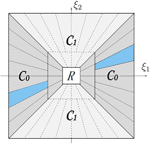
Figure 1. Adaptive conical frequency domain structure of two-scale decomposition; R is the low frequency domain, C0 is the horizontal cone domain, and C1 is the vertical cone domain.

Due to down-sampling, shearlet transform will cause the aliasing of the decomposed sub-band spectrum, resulting in the weakening of direction selectivity and blurring of the image edge. Furthermore, the translation invariance is lost, resulting in the pseudo-Gibbs phenomenon or ringing effect, which affects the denoising effect. NSST uses non-subsampled Laplacian pyramid (NSLP) filters and non-subsampled shear directional filters (SF) to enhance directional selectivity in multi-scale decomposition and directional localization and to obtain translation invariance.

The decomposition process of NSST in the frequency domain consists of two steps: multi-scale decomposition and multi-direction decomposition.

Multi-scale decomposition is realized by the NSLP filter bank. After J-level decomposition, the data matrix was decomposed into a low frequency sub-band and J high frequency sub-bands with the same size as the original data matrix. The multi-directional decomposition is realized by SF filter bank with direction and scale-varying, and the high-frequency sub-bands at each scale are decomposed into different directional sub-bands.

Directional sub-bands ($2^l+2$) can be obtained by l-level directional decomposition of any scale high-frequency sub-band. After J-scale decomposition, a total of ${\sum }_{j=1}^J\left(2^{l_j}+2\right)$ directional subbands can be obtained. $l_j$ denotes the directional shear series of scale j (Feng, 2014). Figure 2 shows the schematic diagram of NSST decomposition at scale J=3.

Figure 2

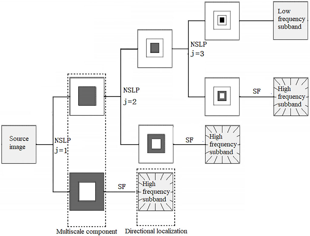
Figure 2. Schematic diagram of NSST three-scale decomposition; NSLP is a non-subsampled Laplacian pyramid filter, SF is a non-subsampled shearlet direction filter, and j is the decomposition scale.

3 Deep learning denoising technology

3.1 FFDNet network

Deep learning has been widely studied in data denoising, but, in most methods, each network is only trained for each specific noise level, such as MLP, CSF, and TNRD. Multiple networks are required for denoising data with different noise levels and cannot deal with spatially varying noise, limiting its application in practical denoising. Zhang (2018) thus proposed a fast and flexible denoising network, FFDNet, which improved DnCNN in four aspects: ① in order to speed up the training and expand the receptive field, the input data are reversibly down-sampled; ② to achieve blind denoising, an adjustable noise level map is added to the input of the network; ③ to improve generalization ability, the orthogonal regularization method is used; ④ residual learning is discarded.

Compared with BM3D and DnCNN_B, FFDNet has three advantages: ① various noise levels of σ∈ [0,75] can be handled using a single network; ② the spatially varying noise can be handled by specifying the non-uniform noise level map; ③ the computational efficiency is higher than that of BM3D.

Figure 3 shows the FFDNet network architecture, consisting of three parts: input, CNN network, and output. ① Input part: the noisy image is reversibly downsampled into four sub-images, which together with the noise level map are used as the input of the CNN. ② CNN consists of three types of convolutional layers. The first is Conv + ReLU, the intermediate multiple layers are Conv + BN + ReLU, and the final layer is the pure convolutional layer Conv. Zero padding is used in each convolutional layer to keep the size of the feature map constant. ③ Output part: the denoising results of four sub-images are reversibly up-sampled to the same size as the noisy image size to be the final denoising result.

Figure 3

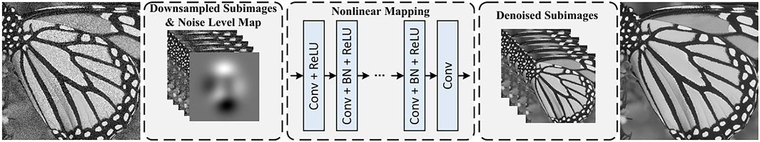
Figure 3. FFDNet network architecture.

In the intermediate multiple convolutional layers, batch normalization (BN) is used to solve the gradient dispersion of the deep network, stabilize the data distribution of each layer, improve the computational efficiency, and reduce the dependence of model parameters on initialization methods.

3.2 ST-hFFDNet network

Figure 4 shows the network architecture of random noise suppression based on NSST and the improved FFDNet.

Figure 4

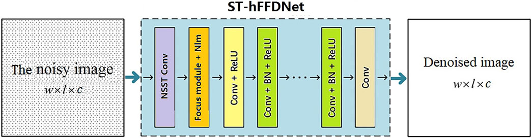
Figure 4. ST-hFFDNet network architecture.

ST-hFFDNet is a deep learning network for image denoising. The denoising principle is as follows. The noisy datasets and clean datasets are decomposed by NSST to obtain sub-band images of different scales and different frequency bands. Based on the convolutional neural network, the complex relationship between the clean and noisy sub-band images with different scales and frequency bands is learned to reconstruct clean images.

The network shown in Figure 4 improves FFDNet in two ways: ① the sub-band images of the noisy image, decomposed by the NSST Convolution module, are used as input to FFDNet. ② The Huber norm is used, which combines MSE (mean squared error) and MAE (mean absolute error). When the residual value is small, MSE is used, and when the residual value is large, MAE is used to reduce the sensitivity to outliers, thereby improving the robustness of the network (Zhang et al., 2020).

Inspired by Zhao et al. (2020), we integrated NSST decomposition and reversible down-sampling processes into CNN as convolution modules, not only streamlining the methodology but also potentially mitigating errors introduced in these steps.

The network has three parts: input, CNN, and output. The input part is the noisy seismic data. The CNN part contains the focus module layer and 13 convolutional layers. The first layer is a NSST convolutional layer, which is composed of 96 3 × 3 × 3 wavelet filters and by which a low-frequency sub-band and multiple high-frequency sub-bands can be obtained. The second layer is a reversible down-sampling layer plus the Nlm (noisy level map) (Focus module+Nlm), which is composed of 385 2 × 2 × 96 wavelet filters. The Focus module slices the sub-band images, and the specific operation is to obtain a value every other pixel in an image, similar to adjacent down-sampling, so that four complementary sub-graphs are obtained without information loss (Glenn Jocher, 2020). The third layer is convolution plus the activation function (Conv+ReLU), which is composed of 96 3 × 3 ×385 convolutional filters and ReLU. The fourth to 13th layers are (Conv+BN+ReLU), which are composed of 96 3 × 3 ×96 convolutional filters, BN, and ReLU. The last layer is a pure convolutional layer (Conv), which consists of three 3 × 3 × 96 convolutional filters. The output of CNN is the final denoised image of size $w\times l\times c$; w and l are the width and height of the sub-band image and c is the number of channels of the noisy image. In this paper, w=100, l=100, and c=3.

In this paper, the BSD500 dataset is used to train the proposed network. First, the dataset is enhanced by flipping, rotating, scaling, cropping, and translation, and the enhanced data set has 4,500 images. Then, the AWGN with noise level σ∈[0,75] is added to the enhanced dataset to obtain the training dataset. The training dataset is decomposed by NSST in three scales and eight directions, and 4,500 low-frequency images and 108,000 high-frequency images with different scales and directions are obtained, which are the same size as the original images. A total of 117,000 training images are obtained, including the original images. In each epoch, 64,000 pairs of size 100 × 100 patches are randomly clipped from these images and corresponding clean images based on the same random seed. The CBSD68 dataset is used to validate the image denoising performance of the proposed method. The validation dataset is obtained by adding AWGN of noise level σ∈[0,75] to the CBSD68 dataset.

The Adam algorithm (Kingma and Ba, 2015) is used to optimize the ST-hFFDNet model by minimizing the loss function (1).

$\begin{array}{l}{L}_{\delta }\left(\mathrm{\Theta },y_i,M_i,x_i\right)=\left\{\begin{array}{c}{\left(F\left(y_i,M_i;\mathrm{\Theta }\right)-x_i\right)}^2,\\ \delta \left|F\left(y_i,M_i;\mathrm{\Theta }\right)-x_i\right|-\frac{1}{2}{\delta }^2,\end{array}|\begin{array}{c}\left|F\left(y_i,M_i;\mathrm{\Theta }\right)-x_i\right|\le \delta \\ \left|F\left(y_i,M_i;\mathrm{\Theta }\right)-x_i\right|\ge \delta \end{array}\right\}\\ L\left(\mathrm{\Theta }\right)=\frac{1}{2N}{\displaystyle \sum _{i=1}^N}{L}_{\delta }\left(\mathrm{\Theta },y_i,M_i,x_i\right),\end{array}(1)$

where M_i is the noise level map, $\mathrm{\Theta }$ is the model weight parameters and bias parameters, y_i is the noisy image, x_i is the clean image, $F\left(y_i,M_i;\mathrm{\Theta }\right)$ is the predicted denoised image, δ is the residual threshold, N is the number of patches randomly clipped in each epoch, $L_{\delta }$ is the Huber norm, and $L\left(\mathrm{\Theta }\right)$ is the loss function.

The setting of hyper-parameters mainly involves the initial learning rate and small batch size. The initial learning rate is set to 10⁻³, and during the training process, Adam adaptively adjusts the learning rate based on the second-order momentum of the gradient. The weights with greater update rate will have a smaller learning rate, and the weights with smaller update rates will have a larger learning rate, both in order to avoid the frequently updated weight parameters being affected by a single abnormal sample and to learn rare sample information at the same time. The mini-batch size is set to 64, and the rest of the hyper-parameters adopt the default setting values of the Adam algorithm. The ST-hFFDNet models are trained in a MATLAB (R2018b) environment with the MatConvNet package and an Nvidia GeForce GTX 1660 GPU. The training of a single model can be done in approximately 15 h.

4 Numerical experimentation

4.1 Linear in-phase axis time profile

Figure 5 shows the comparison of denoising results of the four methods on the simulated data of the linear in-phase axis time profile. The top image in column 1 of Figure 5 is the clean data (2 s on the vertical axis and 500 traces on the horizontal axis), and the other four images, from top to bottom, are with AWGN of σ=30, 50, 70, and 90. The second column of Figure 5 is the local details corresponding to the small blue box in the first column. Columns 3–6 of show the denoising results of NSST, DnCNN, FFDNet, and the proposed method.

Figure 5

Figure 5. Comparison of four denoising methods for the linear in-phase axis time profile; Column 1 of Panel 5 is clean and noisy data (vertical axis time is 2 s, and the horizontal axis track number is 500); Column 2 is the local details corresponding to the small blue box in the first column; Column 3 is the denoising results of NSST; Column 4 is the DnCNN result; Column 5 is the FFDNet result; Column 6 is the proposed method result.

For the case of low noise (σ≤40), as shown in the second row of Figure 5, there is little difference between the four methods from the subjective vision, PSNR (peak signal-to-noise ratio), MSE (mean square error), and SSIM (structural similarity) indicators. However, the denoising effect of the proposed method is better than that of the other three methods, followed by FFDNet, NSST, and DnCNN.

In the case of high noise (σ> 40), as shown in rows three to five of Figure 5, the difference between the four methods is gradually enlarged as the noise increases. The noise level range of DnCNN is [σ≤ 55], and the denoising effect is very good at low noise but becomes very poor at high noise of σ=50; there is almost no denoising effect when σ=90. However, the other three methods have obvious denoising effects on high noise. From the subjective vision and objective indicators (PSNR, MSE, and SSIM), the denoising effect of the proposed method is better than that of the other three methods. The evaluation metrics PSNR, MSE, and SSIM for linear in-phase axis simulation data denoising are shown in Table 1.

Table 1

Table 1. PSNR, MSE, and SSIM after denoising linear in-phase axis simulated data.

4.2 Simulation data on complex inclined fault

Figure 6 compares the denoising results of the four methods on simulated data of the complex inclined fault. The top image in column 1 of Figure 6 is the clean one (2 s on the vertical axis and 200 traces on the horizontal axis), and the other four images, from top to bottom, are those with AWGN of σ=30, 50, 70, and 90. Column 2 shows the local details corresponding to the small green box in the first column. Columns 3–6 show the denoising results of NSST, DnCNN, FFDNet, and the proposed method.

Figure 6

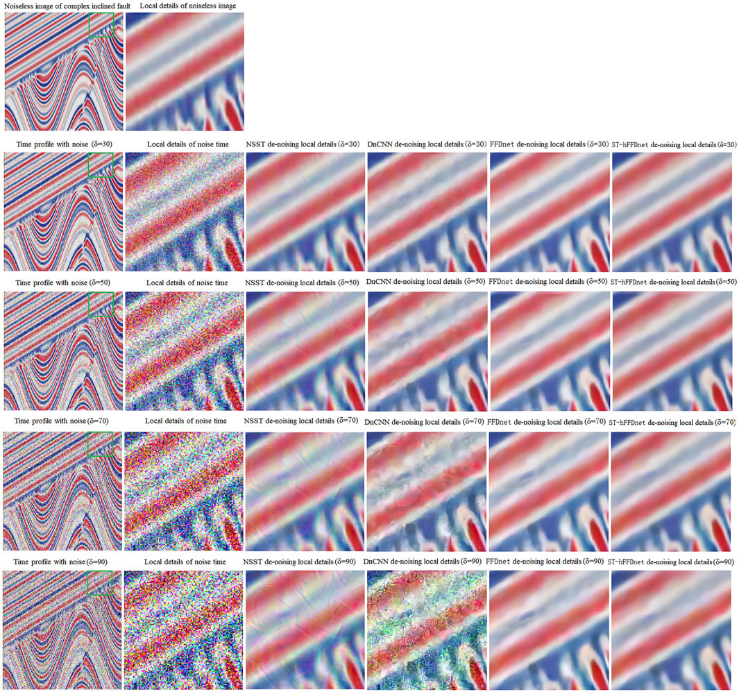
Figure 6. Comparison of the denoising effect of complex inclined fault simulation data; Column 1 of Panel 6 is clean and noisy data (vertical axis time is 2 s, horizontal axis track number is 200); Column 2 is the local details corresponding to the small blue box in the first column; Column 3 is the denoising results of NSST; Column 4 is the DnCNN result; Column 5 is the FFDNet result; Column 6 is the proposed method result.

In the case of low noise (σ≤40) (second row of Figure 6) from subjective vision and objective evaluation indicators (PSNR, MSE, and SSIM), the four methods are still little different, and the denoising effect is, in order, from good to poor: the proposed method, FFDNet, NSST, and DnCNN.

For high noise (σ> 40) (rows three to five of Figure 6), the difference between the four methods increases as the noise increases. When σ=70, the denoising effect of DnCNN is not good, and when σ=90, the denoising effect is very poor. In terms of subjective vision and objective evaluation indicators (PSNR, MSE, and SSIM), the denoising effect of the other three methods is in order from good to poor: the proposed method, FFDNet, and NSST.

PSNR, MSE, and SSIM evaluation metrics are shown in Table 2.

Table 2

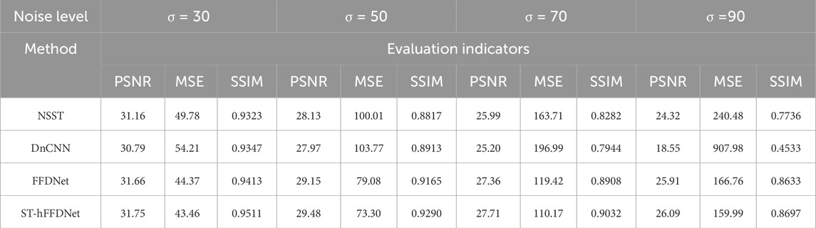
Table 2. PSNR, MSE, and SSIM after denoising simulated data for a complex inclined fault.

Table 3 lists the running time results of DnCNN, FFDNet, and the proposed method for denoising color images with size 256 × 256, 512 × 512, and 1,024 × 1,024. The evaluation was performed in a MATLAB (R2018b) environment on a computer with a four-core Intel(R) Core(TM) i3-10100 CPU @ 3.6 GHz, 16 GB of RAM, and an Nvidia GeForce GTX 1660 GPU. As can be seen from the table, the overall time of DnCNN is about thrice that of the FFDNet method. The running time of the proposed method is generally comparable to that of the FFDNet method.

Table 3

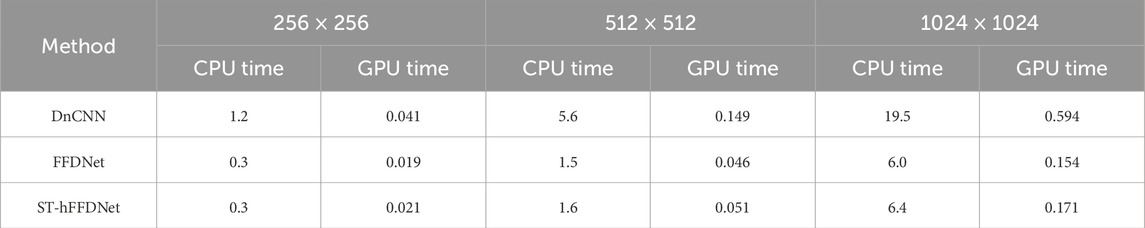
Table 3. Comparison of running time (in seconds) of three deep learning methods for denoising color images with size 256 × 256, 512 × 512, and 1,024 × 1,024.

4.3 Real seismic data

The trained ST-hFFDNet model is used to denoise the real seismic data. Figure 7 compares the denoising effect for real post-stack seismic profile. The first row of Figure 7 shows the post-stack seismic profile and the denoising results of the four methods. The second row is the local detail corresponding to the small blue box in the first row. Rows three to four show the noise removed by the four methods and the local details of the removed noise.

Figure 7

Figure 7. Comparison of the denoising effect for the real post-stack seismic profile.

Row 1 of the figure is the real post-stack seismic profile and denoising results of NSST, DnCNN, FFDNet, and the proposed method. Row 2 is the local detail corresponding to the small blue box in row 1. Row 3 is the noise removed by NSST, DnCNN, FFDNet, and the proposed method. Row 4 is the local noise detail corresponding to the small blue box in row 1.

Column 1 of Figure 7 shows the post-stack seismic profile (top) and local details (bottom). Column 2 is the denoising result of NSST, the local details, the removed noise, and the local details of the removed noise. Column 3 shows the results and details of DnCNN. Column 4 shows the results and details of FFDNet, and Column 5 shows the results and details of the proposed method.

It can be seen from Figure 7 that the denoising results of NSST (column 2), DnCNN (column 3), and FFDNet (column 4) are not obviously different and are slightly blurred. The denoising results of the proposed method (column 5) are significantly improved, and the subjective visual inspection results are better and the details clearer than that of the other three methods.

In addition, from the two aspects of noise removal and preservation of the stratum structure details, we can see from the noise removal of the four methods that: (1) NSST removes certain stratum structure details while de-noising, and its black noise map indicates that the degree of noise removal is lower; (2) DnCNN removes more details of the stratum structure while denoising; (3) FFDNet removes less stratum structure details; (4) the proposed method removes the least stratum structure details while denoising, indicating that the proposed method is better than the other three in denoising and preserving stratum structure details.

Figure 8 shows the denoising results of four methods for linear in-phase axial simulated data and the corresponding amplitude spectra. The upper part of Figure 8, from left to right, is the noisy image, the clean image, and the denoising results of the four methods, respectively. The lower part of Figure 8 is the amplitude spectra corresponding to the upper part. Compared with the amplitude spectrum of the clean image, it is evident that the amplitude spectrum of the proposed method is closest to that of the clean image, the spectrum of FFDNet is slightly inferior to that of the proposed method, the spectrum of NSST is more different than that of the clean image, and the spectrum of DnCNN is the most different to that of the clean image. From PSNR and MSE of four methods, the order in advantage for image denoising is the proposed method, FFDNet, NSST, and DnCNN.

Figure 8

Figure 8. Denoising results of four methods for linear in-phase axial simulated data and corresponding amplitude spectra.

The upper part of Figure 8 is the noisy image (σ=70), the clean image, and the denoising results of NSST, DnCNN, FFDNet, and the proposed method. The lower part is the amplitude spectra corresponding to the upper part.

Figure 9 shows the amplitude spectra of the real post-stack seismic profile. The upper part of Figure 9, from left to right, is the seismic profile and the denoising results of the four methods. The lower part of Figure 9 is the amplitude spectra corresponding to the upper part. From the amplitude spectra, it is evident that the difference among the four methods is not obvious, but the amplitude spectrum of DnCNN is better than that of other three methods. Visually, the order of advantage for the amplitude spectra of the other three methods is the proposed method, FFDNet, and NSST. From a spectra point of view, the superiority of DnCNN over the proposed method and FFDNet may be related to the low noise level of real post-stack seismic profile. Zhang et al. (2018) observed that FFDNet is slightly worse than DnCNN when noise levels are low (σ ≤ 25) but gradually outperforms DnCNN as noise levels increase (σ> 25), which may be due to the trade-off between receptive field size and modeling ability.

Figure 9

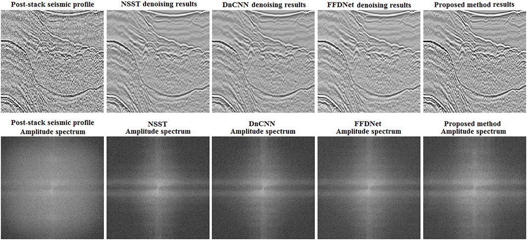
Figure 9. Denoising results of four methods for the real post-stack seismic profile and corresponding amplitude spectra.

The upper part of Figure 9 is the seismic profile and the denoising results of NSST, DnCNN, FFDNet, and the proposed method. The lower part is the amplitude spectra corresponding to the upper part.

Figure 10 shows the change curve of the model loss function with the number of training epochs. As can be seen from the figure, at the beginning of training, the loss function value was 1.35, and after 58 epochs of training, the loss function value dropped to 0.03, with a decline rate of 98%.

Figure 10

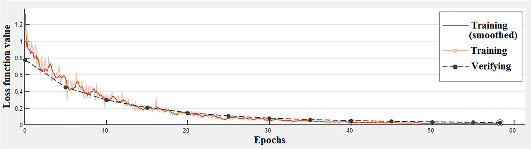
Figure 10. Change of model loss function with the number of training epochs.

5 Conclusion and prospect

The proposed denoising method combines the advantages of NSST, Huber norm, and FFDNet. The seismic signal and random noise are extracted from multi-scale and multi-direction high and low-frequency sub-bands decomposed by NSST, and the joint denoising of multi-scale geometric analysis and deep learning is realized. The joint denoising method can suppress high-frequency noise while retaining more edge details, and the subjective vision and objective evaluation indicators are better than the denoising methods of other multi-scale geometric analyses combined with deep learning. The introduction of BN into the network alleviates the gradient diffusion problem caused by the increase of network layers, and it has been widely used in the field of denoising. The adjustable noise level map can effectively improve the denoising performance of different noise levels, and its blind denoising effect is better than the traditional optimal denoising method BM3D. The Huber norm, introduced into the loss function, can effectively reduce the sensitivity of the network to abnormal data and improve its robustness. The proposed method in this paper involves deep learning, which has shortcomings of depending on large datasets and a time-consuming training process. If the proposed method is combined with transfer learning technology, it can effectively reduce the dependence on large data sets and further improve computational efficiency, which will be our next research direction.

Data availability statement

The raw data supporting the conclusion of this article will be made available by the authors, without undue reservation.

Author contributions

HF: writing–original draft and writing–review and editing. YZ: funding acquisition, supervision, and writing–review and editing. WW: supervision, project administration, and writing–review and editing. TL: writing–review and editing.

Funding

The authors declare that financial support was received for the research, authorship, and/or publication of this article. This research was jointly financed by the Seismotectonic Exploration Project in Henan Province, the Fundamental Research Funds in the Institute of Geology, China Earthquake Administration (IGCEA 2008), the Scientific and technological key project in Henan Province (232102320018), and the Key Programme of Earthquake Emergency for Youths, China Earthquake Administration (CEAEDEM202315).

Conflict of interest

The authors declare that the research was conducted in the absence of any commercial or financial relationships that could be construed as a potential conflict of interest.

Publisher’s note

All claims expressed in this article are solely those of the authors and do not necessarily represent those of their affiliated organizations, or those of the publisher, the editors, and the reviewers. Any product that may be evaluated in this article, or claim that may be made by its manufacturer, is not guaranteed or endorsed by the publisher.

References

Aigu L., (2015). Research on image enhancement methods based on shearlet and NSST transform. Urumqi, Xinjiang: Urumqi Xinjiang University.

Google Scholar

Buades, A., Coll, B., and Morel, J. M. (2005). “A non-local algorithm for image denoising,” in IEEE international conference on computer vision and pattern recognition (Washington DC: IEEE Computer Society), 2, 60–65. doi:10.1109/cvpr.2005.38

CrossRef Full Text | Google Scholar

Dabov, K., Foi, A., Katkovnik, V., and Egiazarian, K. (2007). Image denoising by sparse 3-D transform-domain collaborative filtering. IEEE Transaction Signal Process. 16 (8), 2080–2095. doi:10.1109/tip.2007.901238

PubMed Abstract | CrossRef Full Text | Google Scholar

Feng, Y., and Xue, R. (2014). Advances in theory and application of shearlets. J. Xinyang Normal Univ. Nat. Sci. Ed. 27 (3), 463–468. doi:10.3969/j.issn.1003-0972.2014.03.040

CrossRef Full Text | Google Scholar

Glenn, J. (2020). Ultralytics.

Google Scholar

Guo, K., and Labate, D. (2007). Optimally sparse multidimensional representation using shearlets. SLAM J. Math. Analysis 39 (1), 298–318. doi:10.1137/060649781

CrossRef Full Text | Google Scholar

Guo, K., Lim, W. Q., Labate, D., Weiss, G., and Wilson, E. (2004). Wavelets with composite dilations. Electr Res Announc AMS 10, 78–87. doi:10.1090/s1079-6762-04-00132-5

CrossRef Full Text | Google Scholar

Han, W. F. (2013). Research on Shearlet domain image denoising Algorithm via sparse representation. Guangzhou, Guangdong: South China University of Technology.

Google Scholar

Huang, D. Y. (2018). Research on wavelet neural network denoising based on sampling principle. Chengdu: University of Electronic Science and Technology of China.

Google Scholar

Ian, J. G., Pouget-Abadie, J., Mirza, M., Xu, B., Warde-Farley, D., Ozair, S., et al. (2014). Generative adversarial nets. arXiv:1406.2661v1 [stat.ML]. doi:10.3156/JSOFT.29.5_177_2

CrossRef Full Text | Google Scholar

Kingma, D., and Ba, J. (2015). “Adam: a method for stochastic optimization,” in International conference for learning representations.

Google Scholar

Kong, Z. M., Yang, X. W., and He, L. F. (2020). A comprehensive comparison of multi-dimensional image denoising methods. arXiv:2011, 03462v1. [eess.IV]. doi:10.48550/arXiv.2011.03462

CrossRef Full Text | Google Scholar

Labate, D., Lim, W. Q., Kutyniok, G., and Weissb, B. (2005). Sparse multidimensional representation using shearlets. Bellingham, WA: International Society for Optics and Photonics.

Google Scholar

Li, Y., Wang, S. Q., and Deng, C. Z. (2011). Overview on image denoising based on multi-scale geometric analysis. Comput. Eng. Appl. 47 (34), 168–173. doi:10.3778/j.issn.1002-8331.2011.34.047

CrossRef Full Text | Google Scholar

Liu, D., Jia, J. L., Zhao, Y. Q., and Qian, Y. R. (2021). Overview of image denoising methods based on deep learning. Comput. Eng. Appl. 57 (7), 1–13. doi:10.3778/j.issn.1002-8331.2011-0341

CrossRef Full Text | Google Scholar

Liu, P. J., Zhang, H. Z., Zhang, K., et al. (2018). Multi-level wavelet-CNN for image restoration. arXiv:1805, 07071v2. [cs.CV]. doi:10.1109/CVPRW.2018.00121

CrossRef Full Text | Google Scholar

Liu, X. Z., Hu, T. Y., Liu, T., Wei, Z. F., Xie, F., An, S. P., et al. (2022). Seismic multiple suppression method by using of data augmentation CODEC Convolutional network. Oil Geophys. Prospect. 57 (7), 757–767. doi:10.13810/j.cnki.issn.1000-7210.2022.04.002

CrossRef Full Text | Google Scholar

Lv, Z. Y. (2021). Research on image denoising based on multi-scale geometric decomposition and neural network. Dalian: Dalian University of Technology.

Google Scholar

Ma, K. (2014). Multiscale geometric analysis theory and application research of infrared image. Chengdu: University of Electronic Science and Technology of China.

Google Scholar

Tang, F. (2014). Research on image denoising methods based on contourlet transform and shearlet transform[D]. Xiangtan, Hunan: Xiangtan University.

Google Scholar

Wu, G. N., Yu, M. M., Wang, J. X., and Liu, G. C. (2022). Stationary wavelet transform and deep residual network are used to suppress seismic random noise. Oil Geophys. Prospect. 57 (7), 43–51. doi:10.13810/j.cnki.issn.1000-7210.2022.01.005

CrossRef Full Text | Google Scholar

Zhang, J., Chen, X. H., Jiang, W., Dan, Z. W., Xiao, X., et al. (2020). Seismic wavelet extraction in depth domain based on subspace constrained Huber norm. Oil Geophys. Prospect. 55 (6), 1231–1236. doi:10.13810/j.cnki.issn.1000-7210.2020.06.005

CrossRef Full Text | Google Scholar

Zhang, K., Zuo, W., and Zhang, L. (2018). FFDNet: toward a fast and flexible solution for CNN-based image denoising. IEEE Trans. Image Process. 27 (9), 4608–4622. doi:10.1109/tip.2018.2839891

PubMed Abstract | CrossRef Full Text | Google Scholar

Zhang, K., Zuo, W. M., Chen, Y. J., Meng, D., and Zhang, L. (2017). Beyond a Gaussian denoiser: residual learning of deep CNN for image denoising. IEEE Trans. Image Process. 26 (7), 3142–3155. doi:10.1109/tip.2017.2662206

PubMed Abstract | CrossRef Full Text | Google Scholar

Zhang, M., Liu, Y., and Chen, Y. K. (2019). Unsupervised seismic random noise attenuation based on deep convolutional neural network. IEEE Access 7, 179810–179822. doi:10.1109/access.2019.2959238

CrossRef Full Text | Google Scholar

Zhang, Y., Li, X. Y., Wang, B., Li, J., Wang, H. T., et al. (2022). Robust seismic data denoising based on deep learning. Oil Geophys. Prospect. 57 (1), 12–25. doi:10.13810/j.cnki.issn.1000-7210.2022.01.002

CrossRef Full Text | Google Scholar

Zhao, Y. X., Li, Y., and Yang, B. J. (2020). Denoising of seismic data in desert environment based on a variational mode decomposition and a convolutional neural network. Geophys. J. Int. 221 (2), 1211–1225. doi:10.1093/gji/ggaa071

CrossRef Full Text | Google Scholar