Deep learning for geological mapping in the overburden area

This paper aims to achieve bedrock geologic mapping in the overburden area using big data, distributed computing, and deep learning techniques. First, the satellite Bouguer gravity anomaly with a resolution of 2′×2′ in the range of E66^°-E96^°, N40^°-N55^° and 1:5000000 Asia-European geological map are used to design a dataset for bedrock prediction. Then, starting from the gravity anomaly formula in the spherical coordinate system, we deduce the non-linear functional between rock density ρ and rock mineral composition m, content p, buried depth h, diagenesis time t and other variables. We analyze the feasibility of using deep neural network to approximate the above nonlinear generalization. The problem of solving deep neural network parameters is transformed into a non-convex optimization problem. We give an iterative, gradient descent-based solution algorithm for the non-convex optimization problem. Utilizing neural architecture search (NAS) and human-designed approach, we propose a geological-geophysical mapping network (GGMNet). The dataset for the network consists of both gravity anomaly and a priori geological information. The network has fast convergence speed and stable iteration during the training process. It also has better performance than a single neural network search or human-designed architectures, with the mean pixel accuracy (MAP) = 63.1% and the frequency weighted intersection over union (FWIoU) = 42.88. Finally, the GGMNet is used to predict the rock distribution of the Junggar Basin.

1 Introduction

Cenozoic loose sediments mask the underlying geological information of the underlying bedrock. Using geophysical detection as the forerunner, combined with the constraints of prior geological-geophysical information, the overburden can be well stripped, revealing deep hidden structures and bedrock (Deng et al., 2019). When using the Bouguer gravity anomaly to map the bedrock in the overburden area, it is necessary to separate the gravity anomaly to obtain the residual field of the target depth. We use edge detection technology to obtain the physical boundary of the remaining Bouguer gravity anomaly. Then, the interpreter combined the existing geological prior information and previous interpretation experience to screen each physical property boundary one by one, and infer the corresponding geological body boundary, stratigraphic age, lithology, etc. This problem is summed up in two steps: accurate description of the outline of the geological body; determining which stratigraphic age and lithology the geological body belongs to. The method require very high geological background knowledge of the interpreter. Due to the limitation of the amount of data, it is difficult to integrate the geological and geophysical data of the entire area.

The successful application of artificial intelligence technology in the field of machine vision provides us with a new research idea. Image semantic segmentation is performing a similar task: segmenting the target and then classifying the resulting object at the pixel level. This paper aims to propose an end-to-end convolutional neural network for overburden area mapping using satellite gravity big data and large-scale regional geological information.

2 Geological setting

The Junggar Basin and its surrounding basin-mountain belt are located in the triangle zone of the Kazakhstan plate, the Siberian plate and the Tarim plate. Since the Paleozoic Era, it has undergone tectonic evolutionary processes such as oceanic expansion, subduction and decay of the oceanic shell of the ancient ocean basin, collision, and intraplate movement (Jinyi, 2004; Wenjiao et al., 2006; Jian et al., 2014; Luo et al., 2016). Most of the existing researches have focused on the well-exposed bedrock areas in East and West Junggar. The hinterland of the basin and the shallow cover area between East and West Junggar, which is covered by Middle-Cenozoic loose sediments, have a relatively low level of basic geological work. The lack of basic geological data has caused some important basic geological issues to remain unresolved. Therefore, this paper selects the Junggar Basin as the study area and predicts the overburden area in the hinterland of the Basin through deep neural network, so as to provide a reference for subsequent studies.

3 Methods and data

3.1 Theory

Gravity anomalies are closely related to the density and spatial distribution of the earth’s internal matter. Heck et al. (2007) proposed that in the spherical coordinate system the gravity can be expressed as:

$g=G\rho \underset{v}{\iiint }\frac{{r^{\prime }}^2\left(r-r^{\prime }\cos \psi \right)\cos {\phi }^{\prime }d{r}^{\prime }d{\phi }^{\prime }d{\lambda }^{\prime }}{{\mathcal{l}}^3}(1)$

where $l$ is the Euclidean distance between the observation point P (φ, λ, r) and the source point Q (φ′, λ′, r′); and $\psi$ is the angle between the position vectors of P and Q; G is the gravitational constant, ρ is the density, φ is the latitude, λ is the longitude, and r is the radial distance.

$\mathcal{l}=\sqrt{{r^{\prime }}^2+r^2-2r^{\prime }r\cos \psi }(2)$

$\cos \psi =\sin \phi \sin {\phi }^{\prime }+\cos \phi \cos {\phi }^{\prime }\cos \left({\lambda }^{\prime }-\lambda \right)(3)$

For

$u=\frac{{r^{\prime }}^2\left(r-r^{\prime }\cos \psi \right)\cos {\phi }^{\prime }}{{\mathcal{l}}^3}(4)$

we have

$g=G\rho \underset{v}{\iiint }ud{r}^{\prime }d{\phi }^{\prime }d{\lambda }^{\prime }(5)$

Density ρ can be expressed as a nonlinear function of variables such as rock mineral composition m, content p, burial depth h, rock formation time t, etc.

$\rho =v\left(m,p,h,t\right)(6)$

Inserting Eq. 6 into Eq. 5 yields

$g=G\cdot v\left(m,p,h,t\right)\cdot \underset{v}{\iiint }ud{r}^{\prime }d{\phi }^{\prime }d{\lambda }^{\prime }(7)$

The above integral equation can be abstracted as the following nonlinear functional:

$v=f\left(u,g\right)(8)$

where u is related to the spatial location, g is the gravity anomaly, and v is related to the rock properties. This nonlinear functional defines a nonlinear mapping relationship from the spatial location and gravity anomaly to lithology.

According to the universal approximation theorem (Cybenko, 1989; Hornik et al., 1989), a feedforward neural network with a sufficient number of hidden units and a nonlinear activation function can approximate any Borel function from one finite-dimensional discrete space to another with arbitrary accuracy. In other words, a deep convolutional neural network can be used to approximate the mapping defined in Eq. 8.

In general, a convolutional neural network of depth n can be represented as:

$y=f^{\left(n\right)}\left(f^{\left(n-1\right)}\left(\cdots f^{\left(2\right)}\left(f^{\left(1\right)}\left(x;\theta \right)\right)\right)\right)=f\left(x;\theta \right)(9)$

The data sample x (gravity anomaly) is fed into a cascading n-layer nonlinear transform network to obtain the desired output y (lithologic distribution). The parameter θ is the learning parameter of this nonlinear transformation. We use an optimizing the algorithm to find θ so that the neural network can maximize the approximation of the mapping defined in Eq. 8.

3.2 Gradient-based learning

The parametric model y = f (x; θ) defines a Conditional probability distribution p (y | x; θ). We use the principle of maximum likelihood to estimate it. The maximum likelihood estimator for θ is then defined as

$\begin{array}{l}{\theta }_{ML}=\underset{\theta }{\mathrm{argmax}}{p}_{\mathrm{mod}el}\left(\mathbb{Y}\mathbb{|}\mathbb{X};\theta \right)\\ =\underset{\theta }{\mathrm{argmax}}{\displaystyle \prod _{i=1}^m}{p}_{\mathrm{mod}el}\left(y^{\left(i\right)}|x^{\left(i\right)};\theta \right)\end{array}(10)$

where $\mathbb{X}=\left\{x^{\left(1\right)},\cdots ,x^{\left(m\right)}\right\}$ is a set of m examples. The p_model (y | x; θ) is a parametric family of probability distributions indexed by θ and it maps any configuration x to a real number estimating the true probability p_data (y | x).

The product of many probabilities is prone to numerical underflow, which is not easy to calculate. We observe that the logarithm of the likelihood does not change its arg max, but conveniently transform the product into a summation:

${\theta }_{ML}=\underset{\theta }{\mathrm{argmax}}{\displaystyle \sum _{i=1}^m}\log p_{\mathrm{mod}el}\left(y^{\left(i\right)}|x^{\left(i\right)};\theta \right)(11)$

Dividing by m, we obtain the expectation with respect to the empirical distribution define by the training data as the estimation criterion.

${\theta }_{ML}=\underset{\theta }{\mathrm{argmax}}{\mathbb{E}}_{x\sim {\widehat{p}}_{data}}\log p_{\mathrm{mod}el}\left(y|x;\theta \right)(12)$

Deep neural network learning is estimating the parameter θ using the principle of maximum likelihood. The essence of this optimization problem is to maximize the log-likelihood, that is, to minimize the negative log-likelihood, which is equivalent to minimizing the cross entropy between the empirical distribution defined by the training set and probability distribution defined by model (Goodfellow et al., 2016).

The cost function is given by

$J\left(\theta \right)=-{\mathbb{E}}_{x,y\sim {\widehat{p}}_{data}}\log p_{\mathrm{mod}el}\left(y|x;\theta \right)(13)$

In order to enhance the generalization ability of the neural network and avoid overfitting during the optimization, we add a parameter regularization term to the cost function to obtain a new objective function:

$\stackrel{\sim }{J}\left(\theta ;x,y\right)=-{\mathbb{E}}_{x,y\sim {\widehat{p}}_{data}}\log p_{\mathrm{mod}el}\left(y|x;\theta \right)+\alpha \mathrm{\Omega }\left(\theta \right)(14)$

The problem of minimizing the objective function is a nonconvex optimization problem. This means that we cannot accurately obtain the global optimal solution of the problem. Therefore, deep neural network training uses an iterative, gradient-based optimization method to obtain a local optimal solution that makes the objective function sufficiently small. The stochastic gradient descent (SGD) algorithm is employed to solve the above nonconvex optimization problem.

We decompose the cross-entropy cost function as a sum over training examples of some per-example loss function.

$J\left(\theta \right)=-{\mathbb{E}}_{x,y\sim {\widehat{p}}_{data}}\log p_{\mathrm{mod}el}\left(x^{\left(i\right)},y^{\left(i\right)},\theta \right)=-\frac{1}{m}{\displaystyle \sum _{i=1}^m}\log p_{\mathrm{mod}el}\left(x^{\left(i\right)},y^{\left(i\right)},\theta \right)(15)$

For these additive cost function, the gradient of the cross-entropy cost function is:

${\nabla }_{\theta }J\left(\theta \right)=-\frac{1}{m}{\displaystyle \sum _{i=1}^m}{\nabla }_{\theta }\log p_{\mathrm{mod}el}\left(x^{\left(i\right)},y^{\left(i\right)},\theta \right)(16)$

The above gradient is an expectation that we can approximately estimate using a small set of samples. On each step of the SGD algorithm, we can sample a minibatch of examples $\mathrm{B}=\left\{x^{\left(1\right)},\cdots ,x^{\left(m^{\prime }\right)}\right\}$ drawn randomly from the training set. The estimate of the gradient is formed as

$gradient=-\frac{1}{m^{\prime }}{\nabla }_{\theta }{\displaystyle \sum _{i=1}^{m^{\prime }}}\log p_{\mathrm{mod}el}\left(x^{\left(i\right)},y^{\left(i\right)},\theta \right)(17)$

The stochastic gradient descent algorithm then follows the estimated gradient downhill:

$\theta \leftarrow \theta -\epsilon \cdot gradient(18)$

where ε is the learning rate.

The stochastic gradient descent algorithm is sometimes very slow or unreliable in the learning process. The method of stochastic gradient descent with momentum (SGD with momentum) is designed to accelerate learning (Robbins and Monro, 1951). SGD with momentum can avoid training into saddle points (Lee et al., 2016) and improve network generalization performance (Hardt et al., 2015; Wilson et al., 2017). SGD scales the gradient uniformly in all directions to determine the descending step size, which can be particularly harmful to ill-conditioned problems. Therefore, SGD needs to frequently modify the learning rate according to the actual situation. To address this issue, adaptive methods such as Adam (Kingma and Ba, 2015), Adagrad (Duchi et al., 2011), and RMSprop (Tieleman and Hinton, 2012) have been proposed that adaptively correct the learning rate during training.

Although the convergence speed and generalization ability of Adam and other adaptive methods are better than SGD in the initial stage of training, their performance in the convergence part has stagnated. A more natural strategy is to use the Adam algorithm to initialize the training, which allows the model to converge quickly and then convert to the SGD with momentum when appropriate (Keskar and Socher, 2017).

3.3 Datasets

The satellite Bouguer gravity data are downloaded from the website (https://bgi.obs-mip.fr/data-products/grids-and-models/wgm2012-global-model/) with the resolution of 2′×2′ and the range of E65^°-95^°, N40^°-55^°. We obtained the regional gravity anomaly by upward continuing the satellite Bouguer gravity anomaly (Figure 1A) to 10 km. We subtract the regional field from the total field to obtain the residual gravity anomaly (Figure 1B). Considering that the resolution of the satellite Bouguer gravity anomaly data used in this paper is 2′×2′, the matching 1:5000000 Asia-European geological map (Figure 2) is used as a priori information for data annotation. In order to accurately depict the boundary contours of the geologic body and accurately classify it by stratum, we annotate the training data at the pixel level. The labeling map adopts the index map mode. The specific categories and index values are shown in Table 1.

Figure 1

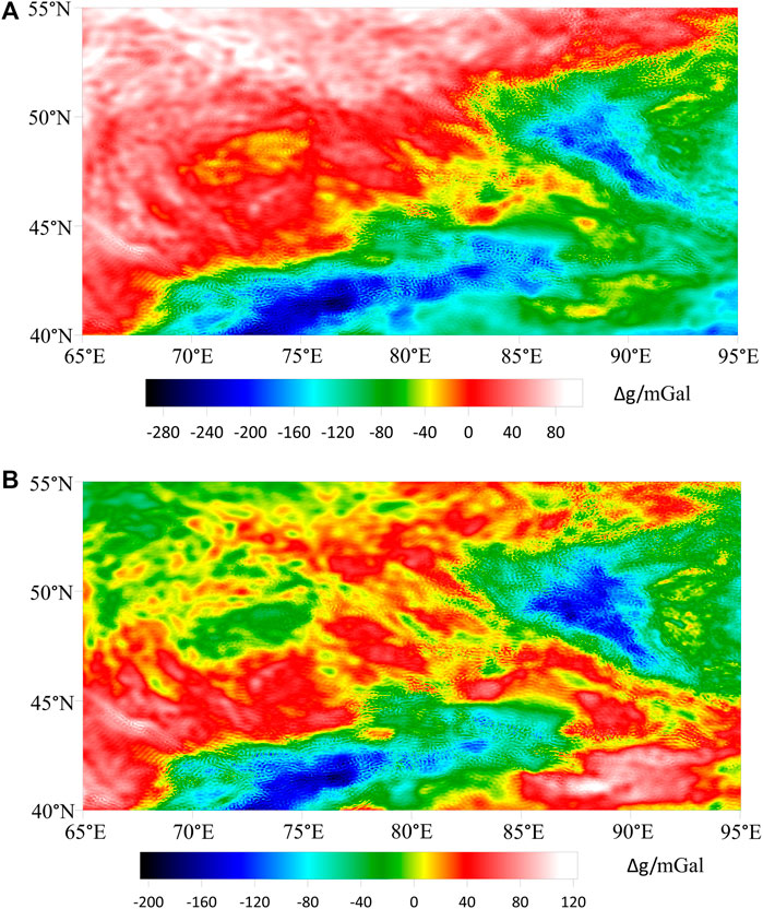
Figure 1. (A) The satellite Bouguer gravity data of the study area with the resolution of 2′×2′ and the range of E65°-95°, N40°-55°. (B) The residual gravity anomaly of the study area: The regional gravity field is obtained by upward continuing the satellite Bouguer gravity data to a depth of 10 km. The residual gravity anomaly is subsequently calculated by subtracting the regional gravity field from the original satellite Bouguer gravity anomaly.

Figure 2

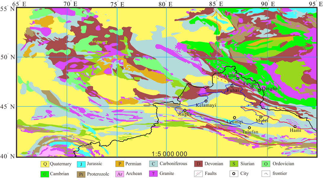
Figure 2. The data annotation of the study area: Considering that the resolution of the satellite Bouguer gravity anomaly data used in this paper is 2′×2′, the matching 1:5000000 Asia-European geological map is used as a priori information for data annotation.

Table 1

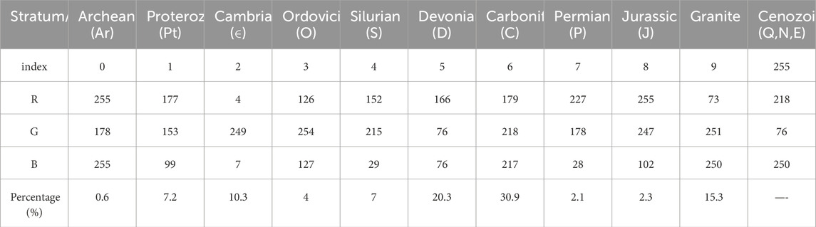
Table 1. Category and index value of annotations.

In order to take into account the semantic segmentation accuracy of both small and large targets and provide more global semantic information to the network, we use a multi-scale sliding window clipping method (Table 2) to clip the data of the entire region. In order to preserve the details of the remaining gravity anomalies, all image sizes are 2048×2048 pixels. A total of 61 samples with bedrock outcrops less than 10% of the total area of the whole map were used as a test set. There are 475 effective samples participating in network training, 15% are randomly selected as the verification set, and the remaining are the training set.

Table 2

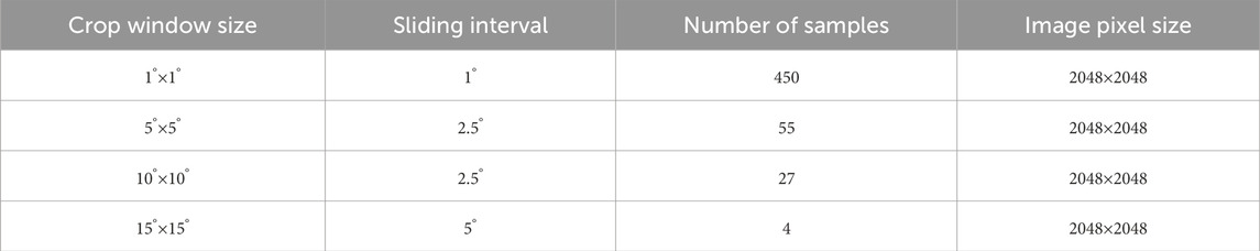
Table 2. Multi-scale sliding window clipping method.

4 Deep convolutional neural network architecture

The general semantic segmentation network mostly pre-trains a backbone on the Imagenet dataset as a feature extractor to obtain the feature map of the image, followed by the feature fusion module and semantic segmentation head to achieve pixel-level segmentation. The shape of satellite gravity anomaly corresponding to each lithology is not the same, but the amplitude is within a certain range. Our segmentation network should not be segmented based on the outline of the target, but rather on the commonality of colors in the same category and the relative position relationship between different categories. In this way, we cannot directly use the existing semantic segmentation network, but should design a personalized network for the task data set.

Manually designing deep neural networks involves the selection of hyperparameters such as the depth of the hidden layer, the width of the network, and the downsampling rate, which is extremely challenging. Neural architecture search (NAS) can help us solve the above problems. Utilizing neural architecture search and human-designed approach, we designed a geological-geophysical mapping network (GGMNet) (Figure 3A).

Figure 3

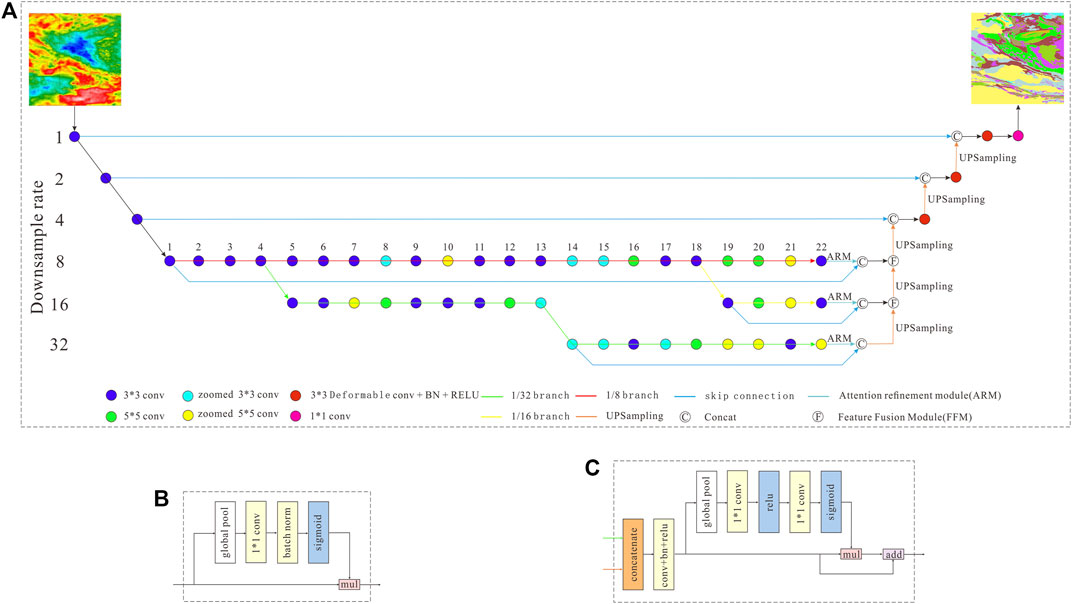
Figure 3. (A) GGMNet Network architecture consists of five modules: A feature encoder to encode the input 3-channel RGB image into a high-dimensional feature map. A multi-resolution feature extraction module (MRFEM) is obtained by searching directly on the target dataset to extract coarse and fine features. Attention Refinement Module is used to refine the features of each stage. A Feature Fusion Module to fuse the features of the three paths. The semantic segmentation module is a matrix with the same size as the original image, and the number of channels is equal to the number of categories. (B) Attention Refinement Module (ARM) employs global average pooling to remove the redundant information of the feature map. (C) Feature Fusion Module: We concatenate branch outputs, apply batch normalization for scale balance, transform to a feature vector via global pooling, and compute a 1x1 convolution-based weight vector for feature re-weighting, effectively selecting and combining features.

4.1 Feature encoder

The feature encoder uses a convolution operation to encode the input 3-channel RGB image into a high-dimensional feature map with 1/8 pixel size and 96 channels (Oktay et al., 2018). It consists of three convolution modules, each of which contains a convolution with the kernel size 3×3 and stride = 2, followed by a batch normalization layer (BN) (Ioffe et al., 2015) and a rectification linear unit (ReLU).

4.2 Multi-resolution feature extraction module

In semantic segmentation task, spatial location information, contextual semantic information, and receptive fields are crucial for segmentation accuracy. The increase of network depth can obtain better contextual semantic information. The skip connections (He et al., 2015; 2016) can enrich spatial location information. The network depth, the size of the convolution kernel, and the position of the skip connections will affect the receptive field of the feature map used for segmentation. Increasing the width of the network can improve the receptive field of the feature map, at the same time, the number of network parameters also increase dramatically. With limited data sets, it is difficult to train a large network with strong generalization capabilities. It is a challenging task to make the network have rich contextual semantic information, precise spatial location information, and sufficient receptive field, which is the ultimate goal of network design.

With the increase of GPU computing power, neural architecture search algorithms are more and more widely used. The Efficientnet (Tan et al., 2019), MobilenetV2 (Sandler et al., 2018), Auto-DeepLab (Liu et al., 2020) are all designed using neural architecture search algorithms. They have achieved good performance in image classification, detection, segmentation and other tasks. We adopt the neural architecture search algorithm (Zoph and Quoc, 2016; Brock et al., 2017; Bender et al., 2018; Pham et al., 2018; Gong et al., 2019) to design multi-resolution feature extraction module. Inspired by Chen, (2019), a multi-resolution feature extraction module (MRFEM) is obtained by searching directly on the target dataset. In order to take into account the experience of manual design and the flexibility of neural architecture search, we designed the search space consists of 5 operators (Table 3).

Table 3

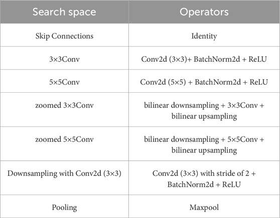
Table 3. Search space and operators.

The zoomed convolution, proposed by Chen, (2019), reduces the size of the input feature map by bilinear downsampling, followed by a convolution operation, and finally restores the output to the original input size by bilinear upsampling. This special design enjoys a lower calculation amount and 2 times larger receptive field compared to standard convolution.

During the neural network search, we fix the network depth of a multi-resolution branch and simultaneously search the paths of three resolution branches with the sampling rates of 1/8, 1/16, and 1/32. For each layer of a single branch, the expansion rate of the network width can be any value in {2, 4, 6, 8}. The operation type can be any one in the search space, and the position of the skip connections can be selected arbitrarily. Since we are more concerned with the accuracy of network segmentation, we use weighted bootstrapped cross-entropy loss function in the search process.

4.3 Attention refinement module

In order to provide the maximum receptive field with global context information, we use Attention Refinement Module (Yu et al., 2018) to refine the features of each stage. Attention Refinement Module (ARM) employs global average pooling to remove the redundant information of the feature map (Figure 3B). It extracts the global context semantic information through the convolution operation with a kernel size of 1×1. The attention vector is calculated through the sigmoid function which is merged into the output to guide the feature learning during the training process.

4.4 Feature fusion module

The features of the three paths are different in level of feature representation. The 1/8 resolution branch represents the relatively macroscopic and superficial semantic information, while the 1/16 and 1/32 resolution branches focus on high-level semantic information such as microscopic details and inter-pixel relationships. Therefore, we cannot simply sum up these features. Moreover, we also need to introduce spatial position information for each resolution branch to achieve precise pixel positioning. We employ the skip connection to integrate the original image information into the output feature map, forming a new feature map that contains rich semantic information and accurate spatial location information. Therefore, we employ a specific Feature Fusion Module (Figure 3C) (Yu et al., 2018) to fuse these features.

We first concatenate the output features of each branch and then utilize the batch normalization to balance the scales of the features. Next, we use global pooling to transform the concatenated feature to a feature vector. We compute a weight vector through the convolution operation with a kernel size of 1×1. The weight vector can re-weight the features, which amounts to feature selection and combination.

4.5 Semantic segmentation head

The output of the semantic segmentation module is a matrix with the same size as the original image, and the number of channels is equal to the number of categories. Each element of the matrix stores the category of the current pixel. A bilinear up-sampling of the feature map after feature fusion is required to restore its size to the original map. We bilinear upsample the 1/8 resolution feature map to 1/4 size, and cascade it with the original 1/4 resolution feature map through a long skip connection. The feature map is sequentially processed with the deformable convolution (Dai et al., 2017) with a kernel size of 3×3, batch normalization layer (BN) and rectification linear unit (ReLU). By doing the same operation on the feature map with 1/4 and 1/2 resolution, the final feature map with the same size as the original pixel is obtained. The network output is converted to pixel classification results by a 1×1 convolution layer.

5 Experiments and discussion

In all experiments, we use Nvidia GeForce GTX 2080Ti GPU, CUDA 10.0, and CUDNN V7. The deep learning framework is PyTorch 1.4.0. Firstly, we introduce the implementation details of GGMNet and the evaluation strategy. We conducted ablation experiments to study the contribution of each component to the network performance. Finally, we compare GGMNet with the current well-performing excellent networks.

5.1 Implementation details

We trained all the models directly on the target data set without pre-training. We initialized the network weight parameters by random initialization. We use 4 GPUs for parallel training, with each card having a batch size of 4 and the training period is 600 epochs. The specific training details are as follows.

5.1.1 Data augmentation

In general, successful neural networks have millions of parameters. It needs a large amount of data to drive the optimization of the network parameters. In reality, there is not as much data as we need. When the training sample is limited, we will adopt a data augmentation strategy during neural network training. Data augmentation can increase the data diversity, prevent overfitting of the training process, and make the neural network robust and generalizable. In this paper, we use random cropping (1,024×1,024), random Gaussian noise (1%–10%), random flip (horizontal, vertical), random rotation (0°–180°), random translation, random contrast increase or decrease (lower=0.5, upper=1.5), and random brightness variation (lower=0.8, upper=1.2).

5.1.2 Loss function

The proportions of the various strata vary considerably in the actual geological problem (Table 1). It leads to a serious category imbalance in the training data. We adopt the weighted bootstrapped cross-entropy loss function to solve the category imbalance problem (Wu et al., 2016; Bulo et al., 2017; Yang et al., 2019). We calculate the category weight w_i based on the proportion of each category in the dataset. Then, we obtain the weighted cross-entropy loss for each pixel and we sort the pixels based on the cross-entropy loss. We only backpropagate the errors in the top-K positions (hard example mining). We set K = 0.15 N, where N is the total number of pixels in the image. Moreover, we weigh the pixel loss based on instance sizes, putting more emphasis on small instances. Specifically, the weighted bootstrapped cross-entropy loss is defined by:

$\mathcal{l}=-\frac{1}{K}{\displaystyle \sum _{i=1}^N}{w}_i\cdot 1\left\{p_{i,y_i}<t_K\right\}\cdot \log p_{i,y_i}(19)$

where y_i is the target class label for pixel i, p_i,yi is the predicted posterior probability for pixel i and class y_i, and 1{x} = 1 if x is true and 0 otherwise. The threshold t_K is the posterior probability of the top-K pixel in descending order according to the loss function.

5.1.3 Learning rate policy

We train the neural network by using both Adam and SGD with momentum. When using the Adam algorithm, we set the initial learning rate lr = 0.001 and the learning rate will be adjusted adaptively during the training. When switching to the SGD algorithm with momentum, the WarmupMultiStepLR learning rate policy is used, with the initial learning rate is the final learning rate of the previous phase, momentum = 0.9, weight_decay = 5e-4. Warmup was performed for the first 5 epochs, after which the learning rate is decreased by a factor of 10 for every 50 epochs.

5.2 Evaluation metrics

For the problem of bedrock prediction in covered areas, which is the focus of this article, it can be formulated as a semantic segmentation task. The metrics employed to evaluate performance include Mean Pixel Accuracy (MPA) and Intersection over Union (IoU). Given the category imbalance present in our dataset, to more objectively assess the network’s predictive efficacy, in addition to the aforementioned evaluation criteria, we use Mean Pixel Accuracy (MPA) and Frequency Weighted Intersection over Union (FWIoU) as the evaluation metrics in order to evaluate the network performance more objectively.

Mean Pixel Accuracy is the average ratio for all categories of samples between the number of correctly classified pixels and the total number of pixels.

$\text{MPA}=\frac{1}{k}{\displaystyle \sum _{i=0}^{k-1}}\frac{p_{ii}}{{\sum }_{j=0}^k{p}_{ij}}(20)$

Where k is the total number of categories; p_ij is the number of pixels of class i but is predicted to be class j.

FWIoU is a weighted summation on the IOU_i of each category and its weight w_i. Where w_i is calculated according to the frequency of each class in the data set.

$\text{IoU}=\frac{\text{area}\left(groundtruth\right)\cap area\left(prediction\right)}{\text{area}\left(groundtruth\right)\cup area\left(prediction\right)}(21)$

$\text{FWIoU}={\displaystyle \sum _{i=0}^{k-1}}{w}_i·{\text{IoU}}_i(22)$

Under the aforementioned training strategy and initial conditions, the proposed GGMNet behaves stably during the training process (Figure 4). At the beginning of training, the Adam algorithm adaptively adjusts the learning rate, the network converges rapidly, the loss function curve decreases linearly (Figure 4A), and the frequency-weighted cross-parallel curve rises rapidly (Figure 4B). When the loss function curve tends to flatten, the optimization algorithm switches to the SGD algorithm with momentum. After many iterations of the network, the FWIoU curve becomes smooth which means that the network performance is almost saturated. It is time to terminate network training.

Figure 4

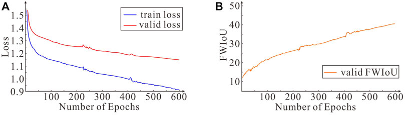
Figure 4. (A) Loss curves of GGMNet on training and validation sets. (B) The FWIoU curve of GGMNet on training and validation sets.

5.3 Results and discussion

5.3.1 Comparison with different depths of the MRFEM

We study the effect of the depth of the multi-resolution feature extraction module on the performance of the neural network, with fixed parameters for the other modules of the network. We set the initial depth to 16, and then increase the depth in increments of 2 until the depth is 24. The experimental results (Table 4) demonstrate that in the depth range of 16–22, the number of parameters in the network increases with depth, and its feature expression ability increases. At this time, the network is able to extract richer feature information, thus significantly improving the network performance. When the network parameters are already sufficient to characterize the dataset, the increase in depth leads to an excess of network parameters. In this case, the dataset cannot drive the network to learn sufficiently, resulting in network underfitting. Therefore, we set the depth of the multi-resolution feature extraction module to 22 layers.

Table 4

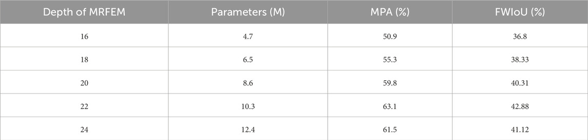
Table 4. The effect of the depth of the MRFEM on the performance of the neural network.

5.3.2 Ablation study for each component in GGMNet

In this subsection, we detailed investigate the effect of each component in our proposed GGMNet step by step. We use the same training strategy to train 600 epochs on five control networks and evaluate the performance of each one on the validation set. We use the U-shape structure (Ronneberger et al., 2015) as our baseline (Table 5a), in which the feature sequentially processed with Encoder, MRFEM, Decoder and a 1×1 convolution layer. The b-d network adds modules in sequence to the baseline.

Table 5

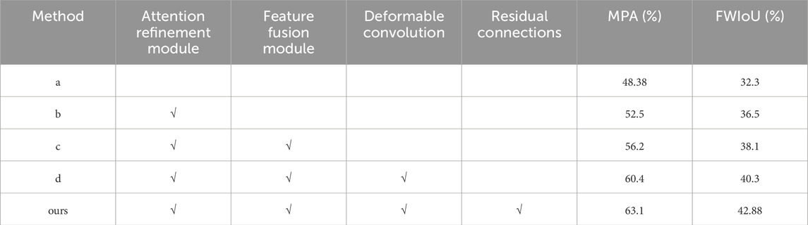
Table 5. Ablation study for each component in GGMNet.

The experimental results (Table 5) demonstrate that the addition of the ARM increases the MPA from 48.38% to 52.5%, and the FWIoU from 32.31% to 36.5%. The FFM enables the network to well integrate features of different resolutions to achieve multi-scale prediction with the MPA is increased by 4.12 and the FWIoU is increased by 1.6. With the addition of deformable convolution, the network’s receptive field is further enlarged, and the description of irregular boundary contours is more accurate. The GGMNet’s performance is greatly improved, with the MPA is increased by 4.2 and the FWIoU is increased by 2.2. The introduction of residual connectivity allows the network to focus on the residuals between input and output during the learning process, without having to fit a large amount of redundant information. It also releases the learning ability of the network, making the network training more stable and faster.

5.3.3 Comparison with state-of-the-arts methods

In order to further validate the performance of the GGMNet on the target dataset, we compared the proposed GGMNet with three state-of-the-arts semantic segmentation networks. Table 6 shows that the performance of the semantic segmentation networks on the target datasets are unsatisfactory, with the MPA less than 60%. The GGMNet, which is designed by utilizing neural architecture search (NAS) and human-designed approach, has fewer parameters than HRNetV1-W32. However, GGMNet has a better performance, with the MPA = 63.1% and the FWIoU = 42.88.

Table 6

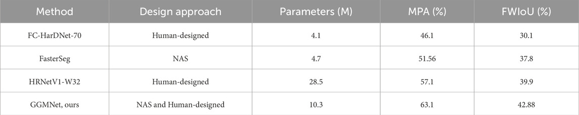
Table 6. Performance comparison of the GGMNet against other state-of-the-arts semantic segmentation networks on the validation set.

Table 7 shows the IoU and MPA of each category on the validation set. The Archean is unable to predict effectively because of the small number of samples. The remaining 9 categories can be successfully predicted by the GGMNet, and the accuracy of the prediction is positively correlated with the number of samples. The experimental results demonstrate the effectiveness and superiority of the neural network design method which performed neural network search directly on the target dataset and followed by manual optimization based on the target task characteristics. GGMNet’s prediction results on the validation set (Figure 5) show that the network has a strong predictive ability especially for categories with a high percentage of pixels. GGMNet can accurately depict the outline of the target body and accurately classify it. Compared with ground truth, the prediction results give richer detailed information.

Table 7

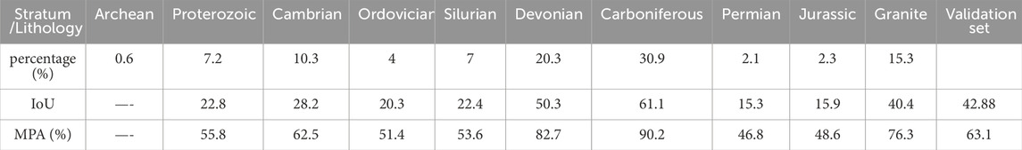
Table 7. The IoU and MPA of GGMNet for each category on the validation set.

Figure 5

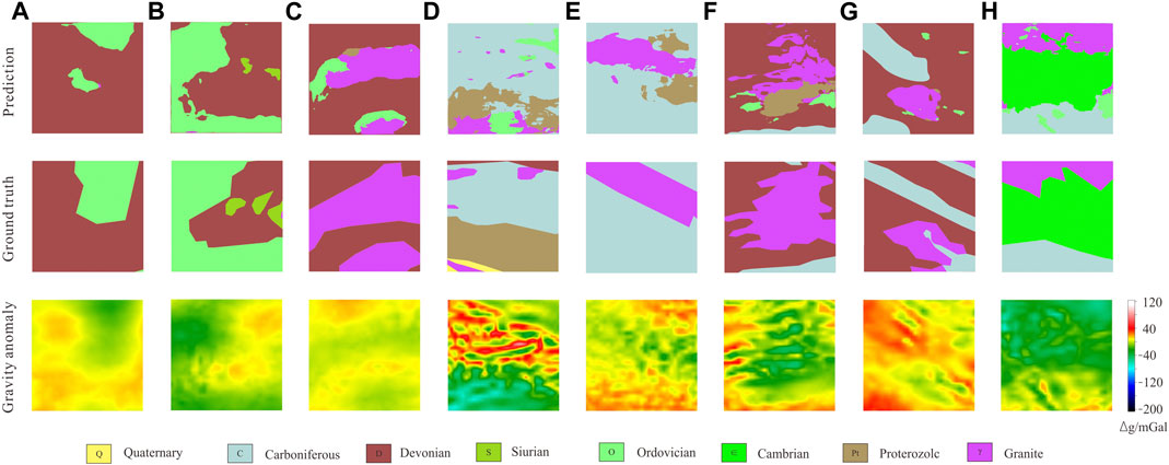
Figure 5. GGMNet’s prediction results on the validation set. First row: the prediction. Second row: ground truth. Third row: the residual gravity anomaly.

5.4 Prediction of Junggar Basin

The residual Bouguer gravity anomalies in the Junggar Basin and its surrounding areas are feed into the trained GGMNet for prediction. Figure 6 is a visualization of the prediction results. In the northern margin of the Junggar Basin, there is a local high gravity anomaly in the south of Fuhai-Fuyun and north of Kelamayi-Mulei. The GGMNet predicts the coexistence of Carboniferous and Devonian strata. The North-East trending Carboniferous and Devonian strata are also widespread in the bedrock outcrops at the periphery of the basin. The local low gravity anomaly is predicted to be granite. In the south of Karamay-Mulei, there is a local negative anomaly area, which is predicted to be Proterozoic, Cambrian strata and Granitic acidic intrusive rocks.

Figure 6

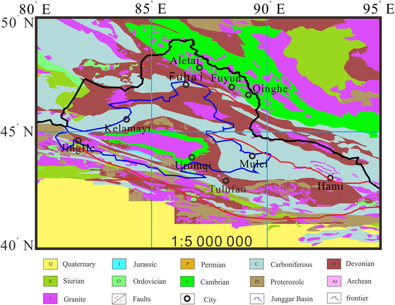
Figure 6. Prediction of Junggar Basin. GGMNet anticipates the presence of both Carboniferous and Devonian formations along the basin’s northern edge, characterized by northeast-oriented outcroppings prevalent in the bedrock perimeter. Areas of diminished gravity are inferred as granite. In the south of Karamay-Mulei, the prediction includes Proterozoic formations, Cambrian strata, and granitic acid intrusion rocks.

Through deep neural network prediction, the distribution of concealed formations or rock bodies throughout the entire Junggar Basin has been ascertained. Within the basin, the major north-northwest trending Kalamayi-Mulei-Hami fault serves as a boundary; to its north, Carboniferous and Devonian strata predominate, while to its south, a mixture of Proterozoic, Cambrian, and Ordovician strata dominate, with acid granite intrusions occurring along the stratigraphic interfaces. The prediction indicates that in the Fuhai area along the northern margin of the Junggar Basin, primarily Carboniferous and Devonian strata are present, intermixed with granitic intrusions. This outcome is consistent with the deep geological structures revealed by traditional geophysical methods.

Studies on the crystalline basement of the Junggar Basin suggest the possible existence of a continental crustal crystalline basement, with its lower portion consisting of strata predating the Neoproterozoic and an upper section characterized by widely distributed Devonian and Carboniferous folded basements. This aligns well with the distribution of concealed geological bodies beneath the Junggar Basin’s cover as predicted by our deep neural network model, indicating a high degree of reasonableness in our predictive results. This concurrence signifies that the predictions made in this study offer a credible depiction of the basin’s sub-surface geology.

6 Conclusion

In this paper, we systematically study the application of deep learning in the overburden area geological mapping, and successfully predict the bedrock of the Junggar Basin by using the satellite Bouguer gravity anomaly and the 1:5000000 Asia-Europe geological map.

Starting from the gravity anomaly formula in the spherical coordinate system, we deduce the non-linear functional between rock density ρ and rock mineral composition m, content p, buried depth h, diagenesis time t and other variables. We analyze the feasibility of using deep neural network to approximate the above nonlinear generalization. The problem of solving deep neural network parameters is transformed into a non-convex optimization problem. We give an iterative, gradient descent-based solution algorithm for the non-convex optimization problem.

We design a dataset for bedrock prediction using both the satellite Bouguer gravity anomaly with a resolution of 2′×2′ in the range of E65^°-95^°, N40^°-55^° and 1:5000000 Asia-European geological map. The dataset contains 536 high-resolution 2048×2048 pixel samples at four scales: 1^°×1^°, 5^°×5^°, 10^°×10^°, and 15^°×15^°.

Utilizing neural architecture search (NAS) and human-designed approach, we propose a deep neural network (GGMNet) for geological mapping. Experiments have demonstrated that our proposed GGMNet has fast convergence and stable iterations during training. GGMNet also has better performance than a single neural network search or human-designed architectures, with the MAP = 63.1% and the FWIoU = 42.88.

Data availability statement

The original contributions presented in the study are included in the article/supplementary material, further inquiries can be directed to the corresponding author.

Author contributions

YL: Conceptualization, Methodology, Writing–original draft. JC: Writing–review and editing. QL: Writing–review and editing. ZL: Writing–review and editing. JL: Writing–review and editing. ZF: Data curation, Writing–review and editing. LZ: Data curation, Writing–review and editing.

Funding

The author(s) declare that financial support was received for the research, authorship, and/or publication of this article. The authors declare financial support was received for the research, authorship, and/or publication of this article. This work was supported in part by the National Key Research and Development Program of China under Grant 2023YFC3008903, and in part by the National Natural Science Foundation of China under Grant 42274184.

Conflict of interest

Authors YL, JC, ZL, and JL were employed by China Coal Technology and Engineering Group Corp.

The remaining authors declare that the research was conducted in the absence of any commercial or financial relationships that could be construed as a potential conflict of interest.

Publisher’s note

All claims expressed in this article are solely those of the authors and do not necessarily represent those of their affiliated organizations, or those of the publisher, the editors and the reviewers. Any product that may be evaluated in this article, or claim that may be made by its manufacturer, is not guaranteed or endorsed by the publisher.

References

Bender, G., Jan Kindermans, P., Zoph, B., Vasudevan, V., and Le, Q. (2018). “Understanding and simplifying one-shot architecture search,” in International Conference on Machine Learning, Stockholm, Sweden, 549–558.

Google Scholar

Brock, A., Lim, T., Ritchie, J. M., and Weston, N. (2017). Smash: one-shot model architecture search through hypernetworks. Available at: https://arxiv.org/abs/1708.05344.

Google Scholar

Bulo, S. R., Neuhold, G., and Kontschieder, P. (2017). “Loss max-pooling for semantic image segmentation,” in CVPR, Honolulu, HI, USA, July, 2017. doi:10.1109/cvpr.2017.749

CrossRef Full Text | Google Scholar

Chen, W., Gong, X., Liu, X., Zhang, Q., Li, Y., and Wang, Z. (2019). FasterSeg: searching for faster real-time semantic segmentation. Available at: https://arxiv.org/abs/1912.10917.

Google Scholar

Cybenko, G. Approximation by superpositions of a sigmoidal function [J]. Math. Control, Signals Syst., 1989, 2(4):303–314. doi:10.1007/bf02551274

CrossRef Full Text | Google Scholar

Dai, J., Qi, H., Xiong, Y., Li, Y., Zhang, G., Hu, H., et al. (2017). Deformable convolutional networks. Available at: https://arxiv.org/abs/1703.06211.doi:10.1109/iccv.2017.89

CrossRef Full Text | Google Scholar

Deng, Z., Meng, G., Tang, H., Yan, J., Qi, G., and Xue, R. (2019). 1:50 000 bedrock geological mapping in shallow overburden area: a case study of kashkeneshakar sheet (L45E009020) on the northern margin of Junggar Basin. Acta Geosci. Sin., (In Chinese with English abstract).

Google Scholar

Duchi, J., Hazan, E., and Singer, Y. (2011). Adaptive subgradient methods for online learning and stochastic optimization. J. Mach. Learn. Res. 12, 2121–2159.

Google Scholar

Gong, X., Chang, S., Jiang, Y., and Wang, Z. (2019). “Autogan: neural architecture search for generative adversarial networks,” in Proceedings of the IEEE International Conference on Computer Vision, Seoul, Korea (South), October, 2019, 3224–3234. doi:10.1109/iccv.2019.00332

CrossRef Full Text | Google Scholar

Goodfellow, I., Bengio, Y., and Courville, A. (2016). Deep learning. Cambridge, Massachusetts, United States: The MIT Press.

Google Scholar

Hardt, M., Recht, B., and Singer, Y. (2015). Train faster, generalize better: stability of stochastic gradient descent. Available at: https://arxiv.org/abs/1509.01240.

Google Scholar

He, K., Zhang, X., Ren, S., and Sun, J. (2015). Deep residual learning for image recognition. Available at: https://arxiv.org/abs/1512.03385.

Google Scholar

He, K., Zhang, X., Ren, S., and Sun, J. (2016). Identity mappings in deep residual networks. Available at: https://arxiv.org/abs/1603.05027.

CrossRef Full Text | Google Scholar

Heck, S. K. (2007). A comparison of the tesseroid, prism and point-mass approaches for mass reductions in gravity field modelling. J. Geodesy 81 (2), 121–136. doi:10.1007/s00190-006-0094-0

CrossRef Full Text | Google Scholar

Hornik, K., Stinchcombe, M., and White, H. (1989). Multilayer feedforward networks are universal approximators. Neural Netw. 2 (5), 359–366. doi:10.1016/0893-6080(89)90020-8

CrossRef Full Text | Google Scholar

Ioffe, S., and Szegedy, C. (2015). Batch normalization: accelerating deep network training by reducing internal covariate shift. Available at: https://arxiv.org/abs/1502.03167.

Google Scholar

Jian, P., Kröner, A., Jahn, B. M., Windley, B. F., Shi, Y., Zhang, W., et al. (2014). Zircon dating of Neoproterozoic and Cambrian ophiolites in West Mongolia and implications for the timing of orogenic processes in the central part of the Central Asian Orogenic Belt. Earth-Science Rev. 133, 62–93. doi:10.1016/j.earscirev.2014.02.006

CrossRef Full Text | Google Scholar

Jinyi, Li (2004). Late Neoproterozoic and Paleozoic tectonic framework and evolution of eastern Xinjiang. Geol. Rev. 50 (3), 304–322. (In Chinese with English abstract).

Google Scholar

Keskar, N. S., and Socher, R. (2017). Improving generalization performance by switching from Adam to SGD. Available at: https://arxiv.org/abs/1712.07628.

Google Scholar

Kingma, D., and Ba, J. (2015). “Adam: a method for stochastic optimization,” in International Conference on Learning Representations (ICLR 2015), San Diego, CA, USA, May, 2015.

Google Scholar

Lee, J., Simchowitz, M., Jordan, M. I., and Recht, B. (2016). Gradient descent converges to minimizers. Berkeley: University of California, 16.

Google Scholar

Liu, C., Chen, L., Schroff, F., Adam, H., and Hua, W. (2020). “Auto-DeepLab: hierarchical neural architecture search for semantic image segmentation,” in 2019 IEEE/CVF Conference on Computer Vision and Pattern Recognition (CVPR), Long Beach, CA, USA, June, 2020.

Google Scholar

Luo, T., Liao, Q. A., Zhang, X. H., Chen, J. P., Wang, G. C., and Huang, X. (2016). Geochronology and geochemistry of carboniferous metabasalts in eastern tianshan, central Asia: evidence of a back-arc basin. Int. Geol. Rev. 58 (6), 756–772. doi:10.1080/00206814.2015.1114433

CrossRef Full Text | Google Scholar

Oktay, O., Schlemper, J., Folgoc, L. L., Lee, M., Heinrich, M., Misawa, K., et al. (2018). Attention U-net: learning where to look for the pancreas. Available at: https://arxiv.org/abs/1804.03999.

Google Scholar

Pham, H., Guan, M. Y., Zoph, B., Le, Q. V., and Dean, J. (2018). Efficient neural architecture search via parameter sharing. Available at: https://arxiv.org/abs/1802.03268.

Google Scholar

Robbins, H., and Sutton, M. (1951). A stochastic approximation method. Ann. Math. statistics 22, 400–407. doi:10.1214/aoms/1177729586

CrossRef Full Text | Google Scholar

Ronneberger, O., Fischer, P., and Brox, T. (2015). “U-net: convolutional networks for biomedical image segmentation,” in International Conference on Medical Image Computing and Computer-Assisted Intervention, Vancouver/Canada, October, 2015, 234–241. doi:10.1007/978-3-319-24574-4_28

CrossRef Full Text | Google Scholar

Sandler, M., Howard, A., Zhu, M., Zhmoginov, A., and Chen, L. C. (2018). “MobileNetV2: inverted residuals and linear bottlenecks,” in 2018 IEEE/CVF Conference on Computer Vision and Pattern Recognition (CVPR). doi:10.1109/cvpr.2018.00474

CrossRef Full Text | Google Scholar

Tan, M., and QuocEfficientnet, V.Le. (2019). Rethinking model scaling for convolutional neural networks. ICML.

Google Scholar

Tieleman, T., and Hinton, G. (2012). Lecture 6.5-RMSProp: divide the gradient by a running average of its recent magnitude. COURSERA Neural Netw. Mach. Learn. 4.

Google Scholar

Wilson, A. C., Roelofs, R., Stern, M., Srebro, N., and Recht, B. (2017). The marginal value of adaptive gradient methods in machine learning. Available at: https://arxiv.org/abs/1705.08292.

Google Scholar

Wu, Z., Shen, C., and van den Hengel, A. (2016). Bridging category-level and instance-level semantic image segmentation. Available at: https://arxiv.org/abs/1605.06885.

Google Scholar

Xiao, W., Windley, B. F., Yan, Q., Qin, K., Chen, H., Yuan, C., et al. (2006). SHRIMP zircon age of the aermantai ophiolite in the north xinjiang area, China and its tectonic implications. Acta Geol. Sin. 80 (1), 32–37. (In Chinese with English abstract).

Google Scholar

Yang, T.-Ju, Collins, M., Zhu, Y., Hwang, J., Liu, T., Zhang, X., et al. (2019). DeeperLab: single-shot image parser. Available at: https://arxiv.org/abs/1902.05093.

Google Scholar

Yu, C., Wang, J., Peng, C., Gao, C., Yu, G., and Sang, N. (2018). BiSeNet: bilateral segmentation network for real-time semantic segmentation. Available at: https://arxiv.org/abs/1808.00897.

CrossRef Full Text | Google Scholar

Zoph, B., and Quoc, V. Le (2016). Neural architecture search with reinforcement learning. Available at: https://arxiv.org/abs/1611.01578.

Google Scholar