Seismic potential in and around the Sichuan basin from the dense GNSS network

The Sichuan basin (SCB) is situated at the southeastern edge of the Tibetan Plateau where widespread seismicity has occurred. In the past decades, seismic events occurred in and around SCB have been responsible for more than 100 thousand casualties. To quantify the present-day seismic hazard of this region, especially the densely populated Chengdu-Chongqing economic zone (CCEZ), we develop a probabilistic earthquake forecast model using strain rates derived from 187 Global Navigation Satellite System (GNSS) horizontal velocities, of which 102 velocity vectors are first released. The second invariant of the strain rate tensor suggests that the Shimian County and its surroundings are exposed to the highest seismic hazard in and around SCB. The second most dangerous area is located between 103–105°E. The Chongqing area is the least dangerous. The principal strain rate axes interior of the Sichuan basin suggest that this region is experiencing broad-scale extension, which according to our knowledge, is first revealed by our dense GNSS network. The comparison between the cumulative histograms of the second invariant of geodetic strain rate and earthquake count indicates that the geodetic strain rates in this region can serve as a reliable predictor of M≥6 earthquake locations. Thus, we proceed to calculate the total seismic moment anticipated for the entire area within the next 30 years.

1 Introduction

The Sichuan basin (SCB), one of the major tectonic elements within the South China block, is located on the southeastern margin of the Tibetan Plateau (Figure 1A). Due to collision between the Tibetan Plateau and the South China block, the SCB and its surroundings have been seismically active, characterized by small-to-medium earthquakes with magnitudes reaching 6.0 (Figure 1B).

As shown in Figure 1B, the SCB is surrounded and sliced by a set of deeply rooted faults that are capable of hosting devastating earthquakes. The Xianshuihe-Xiaojiang fault system (XXFS; Figure 1B) located west of the SCB is regarded as one of China’s most devastating left-lateral strike-slip faults, have caused a minimum of 14 M≥7.0 earthquakes documented since 814 (Allen, et al., 1991; Deng, et al., 2003). The northwestward-dipping Longmenshan fault zone, responsible for the unexpected and destructive 2008 Wenchuan M_w7.9 earthquake, is the most prominent topographic feature in the Sichuan province that separates the cratonic SCB and the eastern margin of the Tibetan Plateau. The southeastward dipping Huayingshan and Lianfeng faults (Le-Tian, et al., 2012), located in the center of SCB, have been the cause of several earthquakes with magnitudes equal to or greater than 5. The most recent of these seismic events is the 2019 Changning earthquake, which had a magnitude of 6.0.

In addition, the SCB is a rather flat terrain that comprises a great part of the Chengdu-Chongqing economic zone (CCEZ; green outline in Figure 1B), a place intensely populated by more than 100 million people. In the past decades, seismic events that occurred in and surrounding SCB have been responsible for more than 100 thousand casualties and considerable destruction. Owing to the limited coverage of the GNSS network in this specific geographical area, previous geodetic investigations have seldom prioritized the assessment of seismic risks in this region. For example, a couple of studies (e.g., Wang et al., 2015; Zheng et al., 2018; Rui and Stamps, 2019a; Wang and Shen, 2020; Stevens and Avouac, 2021) have evaluated the seismic hazards of the mainland China in which the SCB is included, however, due to the limited GNSS dataset, none of these studies have been able to depict the seismic hazards of the SCB in detail. In this work, we aim to finely quantify the seismic hazards of SCB, especially the densely populated CCEZ region, by developing a probabilistic earthquake forecast model, using regional strain rates derived from 187 Global Navigation Satellite System (GNSS) horizontal velocities.

Figure 1

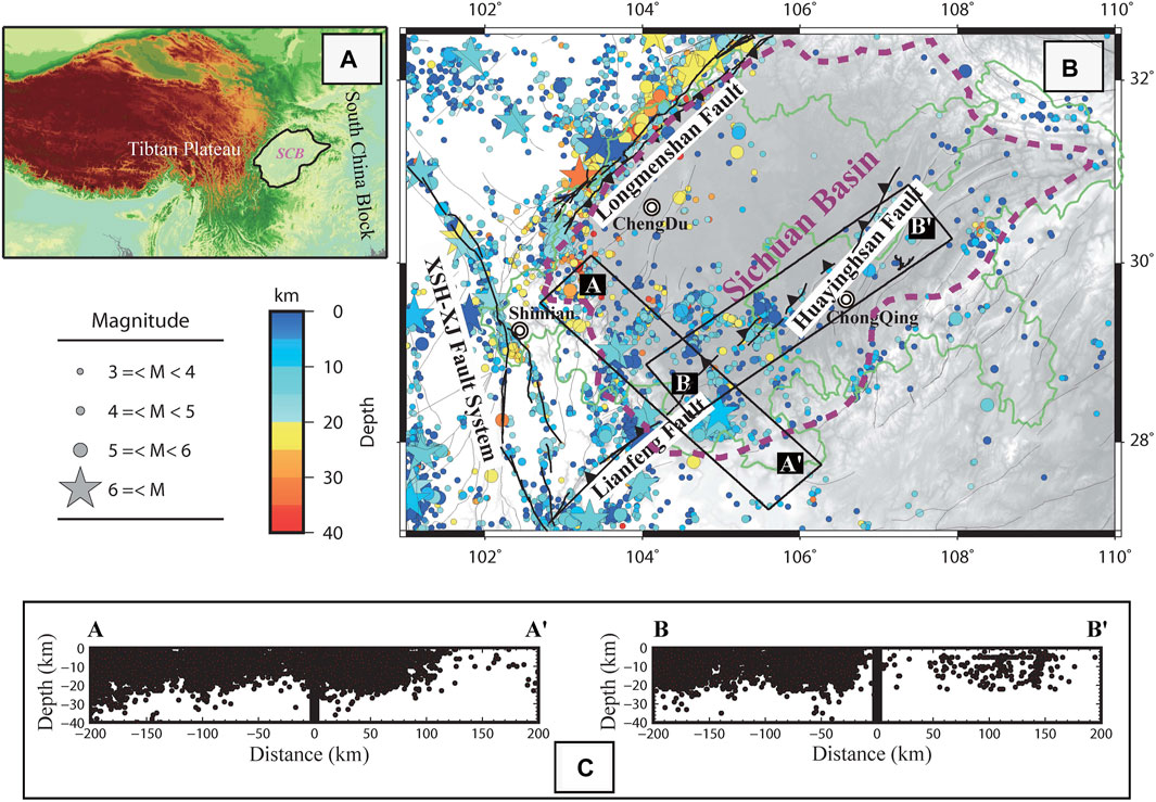
Figure 1. (A). The location of the Sichuan Basin (SCB) with respect to the south China block and Tibetan Plateau. (B). Major faults and historical M≥3 earthquakes since 2000 in the study area. XSH-XJ fault system is short for the Xianshuihe-Xiaojiang fault system Major. The thick brown dashed curve represents the Sichuan Basin (SCB) area. The solid green curves represent the geographic extent of the Chengdu-Chongqing economic zone (CCEZ) which is the main focus of this study. (C). The seismicity-depth distribution of historical earthquakes occurred within profile swaths AA’ and BB’ (Figure 1B) to illustrate the average seismogenic thickness of the region.

2 Dataset

The GNSS sites used in this work are from eight sources: 1) The Crustal Movement Observation Network of China (CMONOC). 2) The GNSS Network of the Sichuan Earthquake Agency. 3) The GNSS Network of the Sichuan Bureau of Surveying, Mapping, and Geoinformation. 4) The Institute of Geophysics of the China Earthquake Administration. 5) The Research Institutes of the China Earthquake Administration. 6) The velocity solution from Li et al. (2023). 7) The velocity solution from Zhang et al. (2013). 8) The GNSS network deployed by Shanghai Huace Navigation Technology Ltd. We note that the raw data from sources six and seven is not accessible.

The GNSS data from sources 1 to 5 and 8 spanning 2011–2023 are processed with the GAMIT-GLOBK processing software (Herring, et al., 2016) following the procedures of McClusky et al. (2000), McCaffrey et al. (2007), and Rui and Stamps (2016). We first combine the phase data of the local GNSS sites with ∼10 continuous IGS sites to estimate loosely constrained positions, with covariance matrices. We then combine these local estimates as “quasi-observations” (Dong, et al., 1998) with the global estimates from the MIT analysis center to transform the positions of local stations into the Eurasian-fixed 2014 International Terrestrial Reference Frame (ITRF 2014) (Altamimi, et al., 2016) and obtain position estimates. We inspect the position time series for each site to identify instrument change related discontinuities as well as earthquake related displacements. We note that, based on the long-term position time series of the continuous GNSS sites (spanning 2011–2023) with discontinuities removed, we see no significant postseismic deformation in this region. This is consistent with the study of Wang and Shen, (2020) which shows that previous devastating earthquakes (including the 2004 Sumatra Mw9.0 earthquake, the 2008 Wenchuan Mw7.8 earthquake, the 2011 Tohoku-Oki Mw9.0 earthquake, and the 2013 Lushan Mw6.7 earthquake) have little impact on GNSS sites in SCB. This result is also consistent with the study of Rui and Stamps (2016) which shows that little postseismic transient deformation is found immediately after the 2008 Wenchuan Mw7.8 earthquake at the continuous GNSS site QLAI which is located in SCB and close to the epicenter.

Realistic uncertainties for the estimated positions and velocities are obtained by adding both white and correlated noise to the phase observations and daily quasi-observations. To do so, we first assign 10 mm for the a priori phase error to make coordinate uncertainties approximately realistic with 2-min sampling following Herring et al. (2016). Second, we remove apparent outliers and down-weight the daily observations for stations and time-periods that reflect a higher than average scatter. Third, we add a random-walk component to all continuous stations that we determined using the first-order Gauss-Markov (FOGMEX) algorithm (Herring, 2003; Reilinger, et al., 2006). Finally, we add an estimate for random-walk noise to the campaign data based on the average of that of the continuous stations and then recalculate the velocity solutions.

The velocity solution from source 6 (Li et al., 2023) was directly combined into our final velocity solution.

The velocities of source 7 (Zhang et al., 2013) were first incorporated by Rui and Stamps (2019b) into the Eurasian fixed ITRF2008 framework. In this study, we further align it to the Eurasian fixed ITRF2014 framework with a rotation pole of (−0.00044 °/Myr, 0.0007 °/Myr, 0.0057 °/Myr) about the X, Y, and Z-axes in an Earth-centered, Earth-fixed coordinate system, as given by the GAMIT-GLOBK program cvframe.

In and surrounding the SCB, we finally derive a velocity solution composed of 587 sites, which is shown in Figure 2, accompanied by a 95% confidence interval (two sigma error for a normal distribution). Out of the total of 587 sites, 187 sites are situated in SCB, and we offer their velocity solutions through the Zenodo repository (https://doi.org/10.5281/zenodo.11203896).

Figure 2

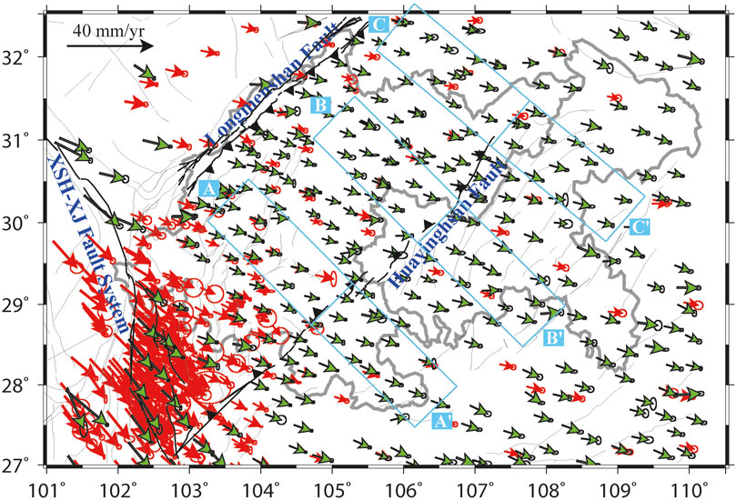
Figure 2. The horizontal GNSS velocity vectors derived by this study. The error ellipses denote the velocity uncertainties under 95% confidence level. The three cyan rectangles labeled as (AA’–CC’) are three velocity profile swaths discussed in section 5.1. The red arrows represent the velocity solution of previously deployed GNSS sites (sources 1–7) and the green arrows represents the velocity solution of the newly deployed GNSS sites by the Shanghai Huace Navigation Technology Ltd. (source 8). For more details, please refer to the main text.

3 Geodetic strain rate

The geodetic strain rate field is derived from the aforementioned GNSS velocity vectors by two steps.

First, to avoid the calculated strain rate field being severely contaminated by any abnormal velocity vectors, we smooth the observed GNSS vectors by employing the gpsgridder script developed by Sandwell and Wessel, (2016). The gpsgridder imposes in-plane vector forces at the selected or all GNSS data locations. These forces deform the elastic body, resulting in a modeled GNSS vector deformation field. The in-plane vector forces are adjusted until the modeled GNSS vector deformation field matches the input GNSS data. To compute a smooth vector velocity field, following Sandwell and Wessel, (2016), we first match 75% of measured GNSS velocity vectors by determining the strength of the body forces at these 75% GNSS locations. Then, the vector velocity field at the rest of the 25% locations is computed from the deformation field imposed by the force vectors at those 75% GNSS locations.

Then, based on the smoothed GNSS velocity field, we calculate the continuous strain rate field by employing the VISR script developed by Shen et al. (2015). The basic idea behind VISR is that, at a given position, the horizontal velocity field in its vicinity is used to estimate the field parameters (including rigid block translation rate, rotation rate, and strain rate components) through a least-squares inversion procedure. At each given position, the weighting function is constructed by taking three factors into account: 1) the GNSS velocity covariance matrix; 2) the distance of the GNSS sites to the interpolation site by employing either a Gaussian ($\exp \left(-∆R^2/D^2\right)$) or quadratic decay function (1/(1+ $∆R^2/D^2$)) where $∆R$ is the distance to the interpolation coordinate R and $D$ is the to-be-estimated optimal spatial smoothing parameter; and 3) the spatial coverage of the GNSS sites by employing an azimuthal weighting function ($n{\theta }_i/4\pi$) or a Voronoi cell areal weighting function ($n{S}_i/{\displaystyle {\sum }_{k=1}^n}{S}_k$) where n is the number of data points selected surrounding R, ${\theta }_i$ is the azimuth span for data point i and $S_i$ is the surface area of the Voronoi cell for the ith data point selected. The optimal solution is determined by comparing the differential strain-rate pattern of two strain-rate fields derived using different weighting schemes following Shen et al. (2015).

4 Geodetic moment rate and seismic potential

To evaluate the seismic potential of the SCB, especially the densely populated area CCEZ, we calculate the second invariant of the strain rate tensor defined as,

${\tau }_{2inv}=\sqrt{{\tau }_e^2+{\tau }_n^2+{2\tau }_{ne}^2}(1)$

Where ${\tau }_e$ and ${\tau }_n$ are the normal strain rate tensors and ${\tau }_{ne}$ the shear strain rate tensor in the east-north Cartesian coordinates (Shen, et al., 2007; Kreemer et al., 2014).

As shown in Figure 3, the maximum second invariant of strain rate, ∼156 nanostrain/yr, is located around Shimian County at the southern end of the Xianshuihe fault (Figure 1). The second largest strain rate area is located between ∼103–105°E. For clarity, we exclude the Shimian area and replot the strain rate (Eq. 1) east of 103°E in Figure 4 with a different color scale from that of Figure 3. It (Figure 4) shows that the average strain rate between ∼103 and 105°E is ∼13.1–18.4 nanostrain/yr and the peak value reaches ∼68 nanostrain/yr. To the east of 105°E, the strain rate is rather slow, most of which are less than 10 nanostrain/yr, corresponding to < 1 mm/yr horizontal velocity gradient within a distance of 100 km.

Figure 3

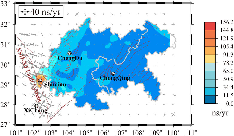
Figure 3. The second invariant of the strain rate tensor. The gray opposing arrows represent the horizontal principal strain-rate axes with a grid resolution of 0.5° × 0.5°.

Figure 4

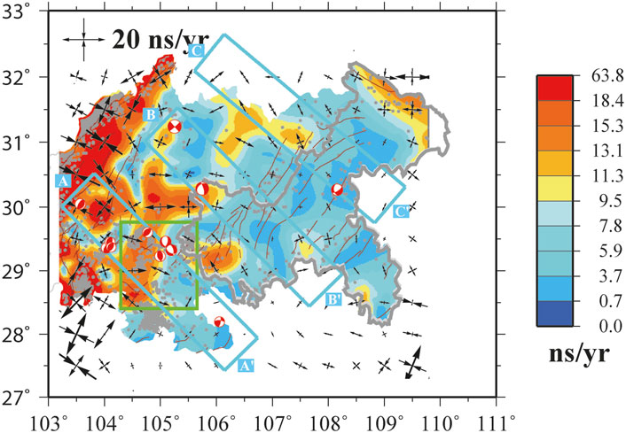
Figure 4. Same as Figure 3 but only show the region east of 103°E. Please note that the color scales in this figure is different from that of Figure 3. The three cyan rectangles are the same velocity profiles (AA’–CC’) defined in Figure 2. The red beach balls are focal mechanisms of historical earthquakes occurred in these three profile swath areas spanning 2009–2017. The green square represents the shale gas mining area.

Besides the second invariant of the strain rate tensor, Figures 3, 4 also show the horizontal principal strain-rate axes (gray and black opposing arrows in Figures 3, 4, respectively) with a grid resolution of 0.5° × 0.5°. The two orientations of the principal strain-rate axes are distinct, unless one of the two principal axes is zero, corresponding to a component of either left or right-lateral slip. Unsurprisingly, Figure 3 shows that the principal strain-rate axes around XXFS are the most prominent in our study area and are dominated by strike-slip motion. To the east of 103°E, Figure 4 shows that the Longmenshan fault is dominated by horizontal compression and the rest of the area, especially the interior of the Sichuan basin (e.g., 104.5–107°E; west of the Huayingshan fault), is dominated by extensional deformation. To verify that such extensional style is not artificial, we calculate strain rates and fault slip rates by evaluating three GNSS velocity profiles (AA’, BB’, and CC’) roughly across the Huayingshan fault defined in Figures 2, 4. Since we are mainly interested in the extensional deformation, we only compare the fault normal components of the GNSS velocity vectors for each profile.

As shown in Figure 5, the weighted mean value of fault normal velocity components on either side of the fault is calculated and depicted as a gray horizontal bar. The height of the gray bar corresponds to its 68% confidence level. It is clearly shown that the fault normal velocity gradients across profiles AA’ (0.73 ± 0.24 mm/yr) and CC’ (1.18 ± 0.38 mm/yr) are positive, suggesting extensional deformation across the whole profile. For profile BB’, the fault normal velocity gradient is positive but insignificant with a 68% confidence level (0.32 ± 0.37 mm/yr). To further verify such conclusion, we calculate a uniform strain rate using all the geodetic data in each profile swath. The derived dilatational strain rates of profiles AA’, BB’, and CC’ are 10.2 ± 4.4, 3.9 ± 6.6, and 5.1 ± 2.8 nanostrain/yr respectively (positive for extension), suggesting again the extensional deformation across the profile swaths AA’ and CC’. Furthermore, we compare our results with the focal mechanisms of historical earthquakes (spanning 2007–2019; https://www.ief.ac.cn/1068/info/2020/21376.html) that fall into the three profile swath areas (Figure 4). It shows that, one normal-faulting event occurred in profiles BB’ and CC’, respectively. For profile AA’, two normal-faulting events occurred in the central area, but other thrust events occurred to the north, suggesting that the strain rate estimates in Figure 5 can only be interpreted as the average deformation rate of all tectonic faults involved in the corresponding profile swath area. We note that such an extensional deformation pattern in the interior of the Sichuan basin is prevalent and, according to our knowledge, first revealed by our dense GNSS network.

Figure 5

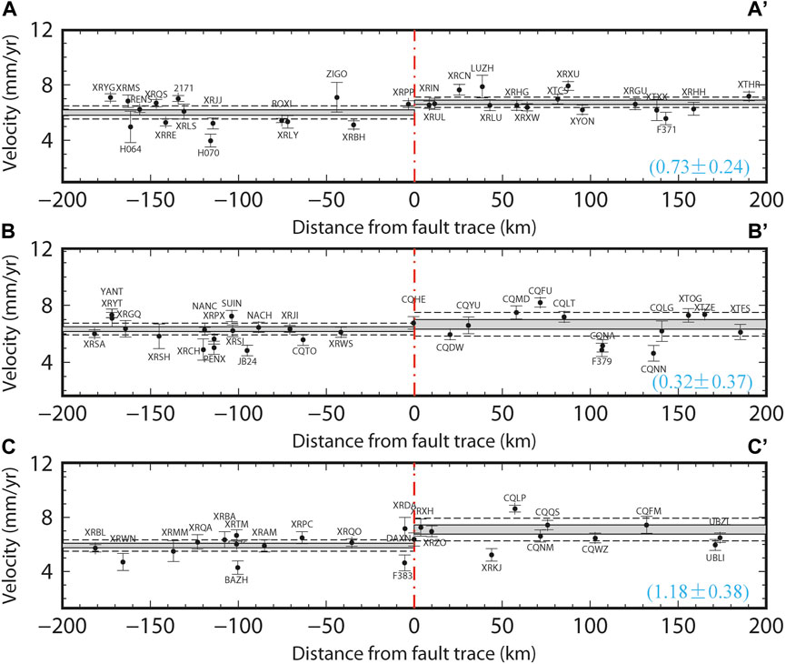
Figure 5. The fault normal components of the 3 GNSS velocity profiles (AA’–CC’) shown in Figures 2, 4. The vertical red dashed line represents the center of the profile which is roughly corresponding to the surficial trace of the Huayingshan fault. The weighted mean value of the velocity vectors on either side of the fault is represented by a gray horizontal bar. The height of the gray bar gives its 68% confidence level. The 95% confidence levels of weighted mean value is depicted as dashed black line.

From a hazard perspective, the strain rates provide an important constraint on expected seismic activity. We follow Savage and Simpson (1997) to calculate a scalar moment rate,

${\dot{M}}_0=2\mu AhMax\left(\left|{\dot{\epsilon }}_1\right|,\left|{\dot{\epsilon }}_2\right|,\left|{\dot{\epsilon }}_1+{\dot{\epsilon }}_2\right|\right)(2)$

where μ and h are the assumed bulk shear modulus (30 Gpa) and seismic thickness (20km; Figure 1C) of the crust. A is the area of the grid cell (0.1° × 0.1°). ${\dot{\epsilon }}_1$ and ${\dot{\epsilon }}_2$ are the principal components of the strain rate tensor, and Max () is a function returning the largest of its arguments.

Assuming that the accumulated seismic moment in each grid cell (0.1° × 0.1°) is going to be released in a single characteristic earthquake (e.g., Kreemer et al., 2014), we then calculate the accumulated moment (Eq. 2) in dyne-cm (10⁻⁷ N-meter) of each grid cell in 30 years and convert it to the equivalent moment magnitude by,

$M_w=2/3\mathit{log}\left(30\times {\dot{M}}_0\right)-10.7(3)$

The derived equivalent moment magnitude of each grid cell (0.1° × 0.1°) is shown in Figure 6. For comparison, we also show the M≥4 historical earthquakes recorded in this region since the year of instrument recording. Similar to the strain rate map in Figure 4, Figure 6 shows that the moment magnitude M_w (Eq. 3) west of 105°E is significantly higher than the eastern region. In addition, to the west of 105°E, most of the M≥4 earthquakes fall into the region with high M_w. However, to the east of 105°E, such a correlation decreases. That is, a portion of M≥4 earthquakes fall outside the region of high M_w. We propose that such low correlation is mainly due to 1) subtle and distributed crustal deformation in this region and 2) the fact that the predictive power of the strain rate model is less sensitive to the small earthquakes (e.g., M≤5) in this region. It is noteworthy that between 105–106°E, there is a shale gas mining area (blue dashed circle in Figure 6) where, due to human activity, some of the non-natural M≥5 earthquakes fall outside the model predicted high M_w region. We note here that the M_w in Figure 6 only represents the 30-year cumulative moment magnitude for the gridded area of 0.1° × 0.1°. However, for a characteristic fault, it always covers an area of more than one grid, so its seismic potential could be even higher. For example, if a fault is 300 km long and 10 km wide, and each grid (0.1° × 0.1° or 10 km × 10 km) covered by this fault can host a M_w6.0 earthquake, then the whole giant fault could host an ∼M_w7.0 earthquake.

Figure 6

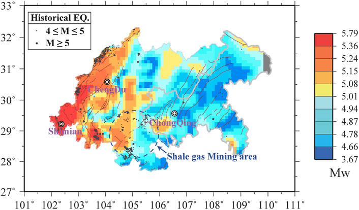
Figure 6. The strain rate model derived accumulative moment magnitude for each grid cell (0.1° × 0.1°) in 30 years. The black dots are the historically recorded M≥4 earthquakes since the year of instrument recording.

We also note that, depending on whether seismic moment is released in a single characteristic earthquake (this study; Figure 6) or follows a Gutenberg-Richter relationship (e.g., Bird et al., 2010; Bird and Kreemer, 2015), the derived hazardous seismic map might be different. For example, for the former (the characteristic earthquake) model, the largest magnitude earthquakes (M_max) are prone to occur in high strain rate areas. However, for the latter (the G-R relationship) model, the locations of the predicted M_max might be less sensitive or even anticorrelated with the magnitude of strain rate (e.g., Stevens and Avouac, 2021) as found in Italy (e.g., Riguzzi et al., 2012) and some stable continental regions (e.g., Calais et al., 2016). In this study, we only focus on the first-order feature of the seismic hazards of the region, that is, the accumulated seismic moment in each gridded cell. How such seismic moment is released in the future (e.g., through the G-R relationship or not) and where the M_max is more likely to occur are beyond the scope of this study.

5 Discussion

We here assess how well the long-term earthquake likelihood is forecasted by the geodetic strain rate derived in Section 4. As suggested by Shen et al. (2007), we compare in Figure 7 the cumulative histograms of the second invariant of geodetic strain rate and earthquake count, with unit areas sorted in decreasing order of strain rate. Theoretically, the two curves should match each other under our assumption that the interseismic geodetic strain is dominantly elastic and released by seismicity in the long run. It can be seen from Figure 7A that, compared to the strain rate forecast, the distribution of the historically recorded M≥5 earthquakes since 26 BC shows relatively fewer events occurring within 25% of the area with higher strain rate (those cumulated on the left side of the vertical bar in Figure 7A) and a better match within the rest of 75% of the area with lower strain rate (those cumulated on the right side of the vertical bar in Figure 7A), indicating that the geodetically derived strain rate field cannot be used as a reasonable forecaster of earthquake locations of the M≥5 earthquakes in the whole study area. We attribute such inconsistency between the geodetic strain rate and distribution of the M≥5 earthquakes to the incompleteness of the earthquake catalog of M≥5, especially prior to the era of instrument recording (Wang, et al., 2015). However, the comparison shown in Figure 7B indicates that the spatial distribution of M≥6 earthquakes since 26 BC correlates much better with the strain rate field, implying that the level of strain rates can be a reasonable forecaster of locations of stronger (e.g., M≥6 instead of M≥5) earthquakes. It is worth pointing out that such positive correlation between the strain rate and earthquake rate is also reported by Wang et al. (2015) and Stevens and Avouac (2021) for the much broader southeastern Tibetan Plateau and India–Asia collision zone. We note that there is a little discrepancy between the earthquake count and strain rate (the earthquake count curve is above the strain rate curve) in Figure 7B around the area of the 25% vertical bar, which might be caused by human activity-induced extra earthquakes in this region. However, such a gap is so small that the predictive power of our strain rate model is still promising.

Figure 7

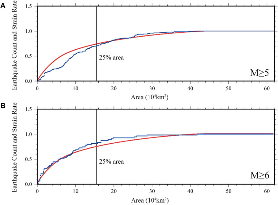
Figure 7. (A) Normalized geodetic strain rate and earthquake count. Red curve is normalized cumulative amount of the second invariant of strain rates in a decreasing order, and blue curve is normalized accumulated earthquake counts of M≥5. (B) Similar as Figure 7A but for the earthquake of M≥6. The vertical bar denotes 25% of the total area measured from origin.

6 Conclusion

To quantify the seismic hazard of SCB, especially the densely populated CCEZ, we have developed a probabilistic earthquake forecast model using regional strain rates derived from 187 Global Positioning System (GPS) horizontal velocities, of which 102 velocity vectors are first released. The second invariant of the strain rate tensor suggests that the Shimian county and its surroundings host the highest seismic hazards in this region. The second most dangerous area is located between 103–105°E (∼13–18 nanostrain/yr) and the Chongqing area is the least dangerous (<10 nanostrain/yr). The principal strain rate axes in the interior of the Sichuan basin suggest that this region is experiencing broad scale extension, which according to our knowledge, is first revealed by our dense GNSS network. The comparison between the cumulative histograms of the second invariant of geodetic strain rate and earthquake count suggests that the geodetic strain rates in this region can be a good forecaster of the locations of M≥6 earthquakes.

Data availability statement

The datasets presented in this study can be found in online repositories. The names of the repository/repositories and accession number(s) can be found below: https://doi.org/10.5281/zenodo.10794282.

Author contributions

RX: Conceptualization, Formal Analysis, Funding acquisition, Investigation, Methodology, Project administration, Validation, Visualization, Writing–original draft, Writing–review and editing. CC: Visualization, Writing–review and editing. FH: Writing–review and editing. XL: Visualization, Writing–review and editing.

Funding

The author(s) declare that financial support was received for the research, authorship, and/or publication of this article. This research was supported by the Science and Technology Department of Sichuan Province (No. 2022JDRC0002), the National Science Foundation of China (42074023), and the Special Fund of the Institute of Geophysics, China Earthquake Administration (DQJB23Z03-05).

Acknowledgments

We thank China Earthquake Administration, Sichuan Bureau of Surveying, Mapping, and Geoinformation and Shanghai Huace Navigation Technology Ltd. for providing access to their data for publication in this manuscript. The figures in this study were generated by the Generic Mapping Tools.

Conflict of interest

The authors declare that the research was conducted in the absence of any commercial or financial relationships that could be construed as a potential conflict of interest.

Publisher’s note

All claims expressed in this article are solely those of the authors and do not necessarily represent those of their affiliated organizations, or those of the publisher, the editors and the reviewers. Any product that may be evaluated in this article, or claim that may be made by its manufacturer, is not guaranteed or endorsed by the publisher.

References

Allen, C. R., Zhuoli, L., Hong, Q., Xueze, W., Huawei, Z., and Weishi, H. (1991). Field study of a highly active fault zone: the Xianshuihe fault of southwestern China. Geol. Soc. Am. Bull. 103 (9), 1178–1199. doi:10.1130/0016-7606(1991)103<1178:fsoaha>2.3.co;2

CrossRef Full Text | Google Scholar

Altamimi, Z., Rebischung, P., Métivier, L., and Collilieux, X. (2016). ITRF2014: a new release of the International Terrestrial Reference Frame modeling non-linear station motions. J. Geophys. Res. Solid Earth 121, 6109–6131. doi:10.1002/2016JB013098

CrossRef Full Text | Google Scholar

Bird, P., and Kreemer, C. (2015). Revised tectonic forecast of global shallow seismicity based on version 2.1 of the Global Strain Rate Map. Bull. Seismol. Soc. Am. 105 (1), 152–166. doi:10.1785/0120140129

CrossRef Full Text | Google Scholar

Bird, P., Kreemer, C., and Holt, W. E. (2010). A long-term forecast of shallow seismicity based on the global strain rate map. Seismol. Res. Lett. 81 (2), 184–194. doi:10.1785/gssrl.81.2.184

CrossRef Full Text | Google Scholar

Calais, E., Camelbeeck, T., Stein, S., Liu, M., and Craig, T. J. (2016). A new paradigm for large earthquakes in stable continental plate interiors. Geophys. Res. Lett. 43, 10621–10637. doi:10.1002/2016GL070815

CrossRef Full Text | Google Scholar

Deng, Q., Zhang, P., Ran, Y., Yang, X., Min, W., and Chu, Q. (2003). Basic characteristics of active tectonics of China. Sci. China Ser. D Earth Sci. 46 (4), 356–372. doi:10.1360/03yd9032

CrossRef Full Text | Google Scholar

Dong, D., Herring, T. A., and King, R. W. (1998). Estimating regional deformation from a combination of space and terrestrial geodetic data. J. Geodesy 72 (4), 200–214. doi:10.1007/s001900050161

CrossRef Full Text | Google Scholar

Herring, T. A., Melbourne, T. I., Murray, M. H., Floyd, M. A., Szeliga, W. M., King, R. W., et al. (2016). Plate boundary observatory and related networks: GPS data analysis methods and geodetic products. Rev. Geophys. 54, 759–808. doi:10.1002/2016RG000529

CrossRef Full Text | Google Scholar

Herring, T. A. (2003). GLOBK: global kalman filter VLBI and GPS analysis program version 10.1 internal memorandum. Cambridge: Massachusetts Institute of Technology.

Google Scholar

Kreemer, C., Blewitt, G., and Klein, E. C. (2014). A geodetic plate motion and global strain rate model. Geochem. Geophys. Geosystems 15, 3849–3889. doi:10.1002/2014GC005407

CrossRef Full Text | Google Scholar

Le-Tian, Z., Sheng, J., Wen-Bo, W., Gao-Feng, Y., and Cheng-Liang, X. (2012). Electrical structure of crust and upper mantle beneath the eastern margin of the Tibetan plateau and the Sichuan basin. Chin. J. Geophys. 55 (12), 4126–4137. doi:10.6038/j.issn.0001-5733.2012.12.025

CrossRef Full Text | Google Scholar

Li, Y., Song, S., Hao, M., Zhuang, W., Cui, D., Yang, F., et al. (2023). Present–day crustal deformation across the Daliang Shan, southeastern Tibetan Plateau constrained by a dense GPS network. Geophys. J. Int. 232 (3), 1619–1638. doi:10.1093/gji/ggac412

CrossRef Full Text | Google Scholar

McCaffrey, R., Qamar, A. I., King, R. W., Wells, R., Khazaradze, G., Williams, C. A., et al. (2007). Fault locking, block rotation and crustal deformation in the Pacific Northwest. Geophys. J. Int. 169 (3), 1315–1340. doi:10.1111/j.1365-246x.2007.03371.x

CrossRef Full Text | Google Scholar

McClusky, S., Balassanian, S., Barka, A., Demir, C., Ergintav, S., Georgiev, I., et al. (2000). Global Positioning System constraints on plate kinematics and dynamics in the eastern Mediterranean and Caucasus. J. Geophys. Res. Solid Earth 105 (B3), 5695–5719. doi:10.1029/1996jb900351

CrossRef Full Text | Google Scholar

Reilinger, R., McClusky, S., Vernant, P., Lawrence, S., Ergintav, S., Cakmak, R., et al. (2006). GPS constraints on continental deformation in the Africa-Arabia-Eurasia continental collision zone and implications for the dynamics of plate interactions. J. Geophys. Res. 111, B05411. doi:10.1029/2005JB004051

CrossRef Full Text | Google Scholar

Riguzzi, F., Crespi, M., Devoti, R., Doglioni, C., Pietrantonio, G., and Pisani, A. R. (2012). Geodetic strain rate and earthquake size: new clues for seismic hazard studies. Phys. Earth Planet. Interiors 206, 67–75. doi:10.1016/j.pepi.2012.07.005

CrossRef Full Text | Google Scholar

Rui, X., and Stamps, D. S. (2016). Present-day kinematics of the eastern Tibetan Plateau and Sichuan Basin: implications for lower crustal rheology. J. Geophys. Res. Solid Earth 121 (5), 3846–3866. doi:10.1002/2016jb012839

CrossRef Full Text | Google Scholar

Rui, X., and Stamps, D. S. (2019a). Strain accommodation in the Daliangshan Mountain area, southeastern margin of the Tibetan Plateau. J. Geophys. Res. Solid Earth 124, 9816–9832. doi:10.1029/2019JB017614

CrossRef Full Text | Google Scholar

Rui, X., and Stamps, D. S. (2019b). A geodetic strain rate and tectonic velocity model for China. Geochem. Geophys. Geosystems 20 (3), 1280–1297. doi:10.1029/2018gc007806

CrossRef Full Text | Google Scholar

Sandwell, D. T., and Wessel, P. (2016). Interpolation of 2-D vector data using constraints from elasticity. Res. Lett. 43, 10703–10709. doi:10.1002/2016GL070340

CrossRef Full Text | Google Scholar

Savage, J. C., and Simpson, R. W. (1997). Surface strain accumulation and the seismic moment tensor. Bull. Seismol. Soc. Am. 87 (5), 1345–1353. doi:10.1785/bssa0870051345

CrossRef Full Text | Google Scholar

Shen, Z. K., Jackson, D. D., and Kagan, Y. Y. (2007). Implications of geodetic strain rate for future earthquakes, with a five-year forecast of M5 earthquakes in southern California. Seismol. Res. Lett. 78 (1), 116–120. doi:10.1785/gssrl.78.1.116

CrossRef Full Text | Google Scholar

Shen, Z. K., Wang, M., Zeng, Y., and Wang, F. (2015). Optimal interpolation of spatially discretized geodetic data. Bull. Seismol. Soc. Am. 95, 686–700. doi:10.1785/0120140247

CrossRef Full Text | Google Scholar

Stevens, V. L., and Avouac, J. P. (2021). On the relationship between strain rate and seismicity in the India–Asia collision zone: implications for probabilistic seismic hazard. Geophys. J. Int. 226 (1), 220–245. doi:10.1093/gji/ggab098

CrossRef Full Text | Google Scholar

Wang, F., Wang, M., Wang, Y., and Shen, Z. K. (2015). Earthquake potential of the Sichuan-Yunnan region, western China. J. Asian Earth Sci. 107, 232–243. doi:10.1016/j.jseaes.2015.04.041

CrossRef Full Text | Google Scholar

Wang, M., and Shen, Z.-K. (2020). Present-day crustal deformation of continental China derived from GPS and its tectonic implications. J. Geophys. Res. Solid Earth 125, e2019JB018774. doi:10.1029/2019JB018774

CrossRef Full Text | Google Scholar

Zhang, Z., McCaffrey, R., and Zhang, P. (2013). Relative motion across the eastern Tibetan Plateau: contributions from faulting, internal strain and rotation rates. Tectonophysics 584, 240–256. doi:10.1016/j.tecto.2012.08.006

CrossRef Full Text | Google Scholar

Zheng, G., Lou, Y., Wang, H., Geng, J., and Shi, C. (2018). Shallow seismicity forecast for the India-Eurasia collision zone based on geodetic strain rates. Geophys. Res. Lett. 45 (17), 8905–8912. doi:10.1029/2018gl078814

CrossRef Full Text | Google Scholar