 Wei Wei
 Yanlin Shao
 Zhonggui Hu
 Qing Wang
 Fan Deng
94% of researchers rate our articles as excellent or good
Learn more about the work of our research integrity team to safeguard the quality of each article we publish.
Find out more
ORIGINAL RESEARCH article
Front. Earth Sci., 11 June 2024
Sec. Geochemistry
Volume 12 - 2024 | https://doi.org/10.3389/feart.2024.1401026
This article is part of the Research TopicUnconventional Resources: Provenance Analysis, Sediment Transport, Reservoir Evaluation, Geo-energyView all 29 articles
Accurately estimating the dolomite content in carbonate rocks is crucial for optimizing oil and gas exploration and production strategies. Hyperspectral techniques for estimating dolomite content have advantages in terms of efficiency, cost-effectiveness, and non-destructiveness compared with traditional laboratory methods. Despite the abundance of hyperspectral data, feature selection and extraction remain challenging. In this study, hyperspectral data collected from surface outcrop in the field using the analytical spectral device (ASD) were applied to construct model for estimating dolomite content. Firstly, the data were preprocessed via outlier analysis and continuum transformation. Next, a hybrid approach integrating spectral knowledge with machine learning was proposed and applied to facilitate efficient and precise feature selection of the hyperspectral data; in this approach, preliminary screening based on spectral knowledge is followed by further hyperspectral data feature selection using a random forest algorithm. The selected features were then combined using a support vector regression algorithm to obtain the estimation model. Finally, the accuracy of the model was evaluated using the hyperspectral data from field outcrop samples. To further verify the effectiveness of this method, various combinations of eight input variables and four machine learning algorithms were compared. Among all combinations, our model achieved the highest accuracy with a test R2 value of 0.91 and a root-mean-square error of only 0.122. The proposed method is practical and efficient and provides precise quantitative data for field geologists to identify the mineral distribution in outcrops. Thus, our method provides robust support for understanding reservoir characteristics and has significant practical value in geological surveys and mineral exploration.
Carbonate rocks are significant reservoir rocks that account for approximately 50% of petroleum reserves worldwide (Gaffey, 1987). Dolomite, one of the key mineral components in carbonate rocks, is an important indicator for assessing reservoir quality, understanding the Earth’s historic climate, and current climate changes. Traditional methods for analyzing dolomite content, which include X-ray diffraction (XRD), scanning electron microscopy (SEM), differential thermal analysis (DTA), thin-section analysis and staining, are primarily laboratory based. These methods are costly, time-consuming, and not suitable for real-time field applications. By contrast, hyperspectral techniques, effectively utilize the spectral differences between minerals for mineralogical analysis (van der Meer et al., 2012; Hecker et al., 2019). Thus, hyperspectral approaches have advantages in terms of speed, efficiency, cost, and non-destructiveness (Zaini et al., 2014; Hamedianfar et al., 2023). Commonly used hyperspectral devices for outcrop studies include ground-based hyperspectral imagers and field spectrometers, such as analytical spectral devices (ASD). ASD spectrometers are particularly favored for their portability and fine spectral resolution, which make them suitable for field analysis of rock mineral content. The unique advantages of hyperspectral analysis are related to the ability to provide abundant information. However, this also presents significant challenges for subsequent data processing and analysis (Rasti et al., 2020; Deepa et al., 2023).
Methods for estimating mineral content based on hyperspectral data can be primarily categorized into two groups: spectral knowledge-based and machine learning-based approaches. Spectral knowledge-based methods focus on extracting a limited but highly representative set of feature bands according to specific rules derived from the spectral characteristics of rocks or minerals. Statistical methods such as linear regression are then used for estimation. These hyperspectral techniques involve selecting mineral diagnostic bands, constructing features such as band ratio, mineral indices through various algebraic operations (Haest et al., 2012; Seo et al., 2023), and analyzing local waveform features including depth, width, symmetry, and area (Hebert, 2019; Kurz et al., 2022; Tan et al., 2023). These spectral knowledge-based methods effectively reduce the dimensionality of hyperspectral data and have clear physical and chemical significance (Kurz et al., 2012; Okyay et al., 2016). However, spectral knowledge-based methods depend significantly on substantial expert knowledge, particularly when constructing complex features like mineral spectral indices. A lack of expert knowledge could result in the omission of critical features, thereby adversely affecting the precision of the outcomes. In addition, these methods are typically used in conjunction with linear regression models, resulting in suboptimal performance when addressing nonlinear issues.
An alternative approach involves the integration of machine learning with hyperspectral data. Machine learning-based methods involve two key steps: feature selection/extraction and machine learning modeling. During feature selection/extraction, feature selection techniques preserve the physical characteristics of the original data and provide strong interpretability, making them popular for reducing the dimensionality of the hyperspectral data analysis. Feature selection techniques mainly include filter, wrapper, and embedded approaches. Filter methods select bands based on specific measurement criteria, such as correlation, information divergence, entropy, and mutual information (Zhou et al., 2022; Tan et al., 2023). Wrapper techniques select features by exploring various feature subsets and evaluating model performance; this process is independent of the model training. Embedded approaches are integrated with certain machine learning algorithms, including random forest (RF) and support vector machine (SVM), often have inherent evaluation metrics to select optimal features (Thomas and Gupta, 2020). Due to their consideration of training samples and feature interdependencies, embedded approaches typically yield superior model performance compared with other feature selection methods (Kumar, 2014; Thomas and Gupta, 2020). Algorithms frequently used in the modeling stage include partial least squares regression (PLSR) (Knox et al., 2015), ensemble learning (Carranza, 2015; Tan et al., 2020; Lin et al., 2022), SVM (Iglesias, 2020; Chatterjee et al., 2022), artificial neural networks (ANN) (Saikia et al., 2020), and deep learning (Zhang T. et al., 2023). Nonlinear models are widely regarded to outperform linear models in a variety of instances (Zhou et al., 2021; Sim et al., 2023). However, the significant potential of deep learning in geochemical analysis is currently hindered by limitations in data quantity (He et al., 2022; Dawson et al., 2023). The benefits of machine learning-based techniques are their powerful data processing and analytical capabilities, impressive analytical speed, independence from expert knowledge, and proficiency in addressing nonlinear challenges (Rodriguez-Galiano et al., 2018; Shirmard et al., 2022). Nonetheless, it is important to note that the efficacy of machine learning is highly correlated with the quality of the input features (Jia et al., 2013; Zhang Y. et al., 2023).
In this study, we propose a scheme for estimating dolomite content in carbonate rocks based on a combination of spectral knowledge and machine learning. This proposed method combines the advantages of spectral knowledge and machine learning to significantly improve the quality of the input data used in machine learning models. Moreover, our method preserves the advantages of machine learning-based approaches, allowing to effectively address nonlinear problems. The main contributions of this study are:
(1) Providing an efficient mechanism for hyperspectral feature selection. The hybrid method for feature selection is characterized by high accuracy, robust interpretability, and low computational cost
(2) Developing a scheme for estimating mineral content based on ASD spectral data. The scheme described in this article covers the entire process from data preprocessing to feature selection and modeling. This method offers a practical and efficient approach for on-site mineral content estimation.
The study area lies in the eastern and northwestern regions of the Sichuan Basin, a substantial oil and gas basin in southwestern China. This basin is positioned to the northwest of the Yangtze platform. The stratigraphy of the Sichuan Basin is both comprehensive and diverse. From the Sinian to the Middle Triassic, the primary depositional environment was marine and dominated by carbonate rocks, By contrast, from the Upper Triassic to the Quaternary, terrestrial deposition primarily involved clastic rocks. This study primarily focuses on the marine sediments from the Sinian to the Triassic, which predominantly comprise carbonate rocks. To ensure sample representativeness, nine outcrops were selected as sampling sites, the specific locations of the sampling sites are depicted in Figure 1.
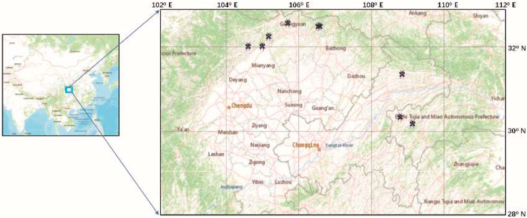
Figure 1. Study area, nine outcrops as our sampling sites (map source provided by ArcGIS online).
Data acquisition for this study comprised two tasks: fieldwork and laboratory work. Fieldwork encompassed three procedures: selecting the sampling locations, collecting hyperspectral data, and gathering rock samples. To enhance the applicability of the model in predicting dolomite content in field outcrops, the hyperspectral data of the training samples were collected on-site in the field. The mineral content of the training samples, which serve as labels for the training data, is ascertained through chemical analysis conducted in the laboratory. The detailed data acquisition process is as follows:.
(1) Selecting field sampling locations. Due to the complex surface conditions of the outcrops (e.g., varying degrees of weathering, smoothness, and the practicality of measuring rock samples), selecting sampling points requires careful consideration. Areas with minimal weathering and relatively smooth, flat surfaces were prioritized for sampling (Figure 2A).
(2) Collecting hyperspectral data. Hyperspectral data were collected using the Analytical Spectral Devices (ASD) FieldSpec3 Hi-Res spectrometer equipped with a contact probe and an integrated light source to minimize the effects of stray light. During field data collection, the spectrometer contact probe was aligned vertically with respect to the sampling point on the outcrop surface, as shown in Figure 2B. The spectral range was between 350 and 2,500 nm, and the spectral resolutions were 3 nm at 700 nm, 10 nm at 1,400 nm, and 10 nm at 2,100 nm. Each sampling point was measured three times, with each comprising an average of 10 scans. All data were subsequently averaged to obtain the final spectrum for that rock sample. A white reference panel was used for calibration every 5 min during the sampling process (Asadzadeh and Souza Filho, 2016).
(3) Gathering rock samples. Following the collection of field hyperspectral data, rock samples were chiseled from the sampling sites using a hammer (Figure 2C). The rock samples were then packed in bags and transported back to the laboratory for analysis (Figure 2D).
(4) Laboratory analysis: XRD analysis was conducted to determine the mineral compositions of the rock samples. The rock samples were ground into powders and analyzed using a SmartLab X-ray diffractometer.
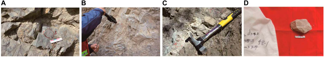
Figure 2. (A) One sample site (B) Field hyperspectral data collection (C) Rock sample collection location (D) One rock sample.
In this study, 206 carbonate rock samples were collected, and detailed mineral content data were obtained for each sample. The collected data were divided into two parts: one part was used for training the model, and the other part was used to validate the model and assess its accuracy.
In this study, the data preprocessing involved outlier analysis and continuum removal. During the acquisition of field hyperspectral data, outliers may arise due to a variety of factors including mishandling, inadequate proximity of the instrument probe to the outcrop surface, and sensor malfunctions. These outliers have the potential to result in overfitting or underfitting by the machine learning algorithms, affecting the efficacy of the model. For outlier analysis, the mean spectrum was calculated for each band ±2 standard deviations for all samples. If 80% of the sample spectral value fell outside of this range, the sample was considered an outlier and removed.
After outlier deletion, continuum removal was executed to suppress the effect of background noise and accentuate subtle spectral variations (Clark and Roush, 1984; Baugh et al., 1998). The continuum removal method applied in this study was based on the approach proposed by Clark and Roush (1984). In addition to enhancing differences, the continuum removal process also normalized the data, facilitating comparison between different spectral curves.
MSK-based feature selection relies on mineral diagnostic bands. The diagnostic bands of dolomite in the near-infrared region are primarily attributed to the energy produced by the vibrations of atoms deviating from their equilibrium positions within the carbonate molecular group (Clark et al., 1990). Specifically, these bands are produced by overtones or combinations of the three fundamental vibration modes of
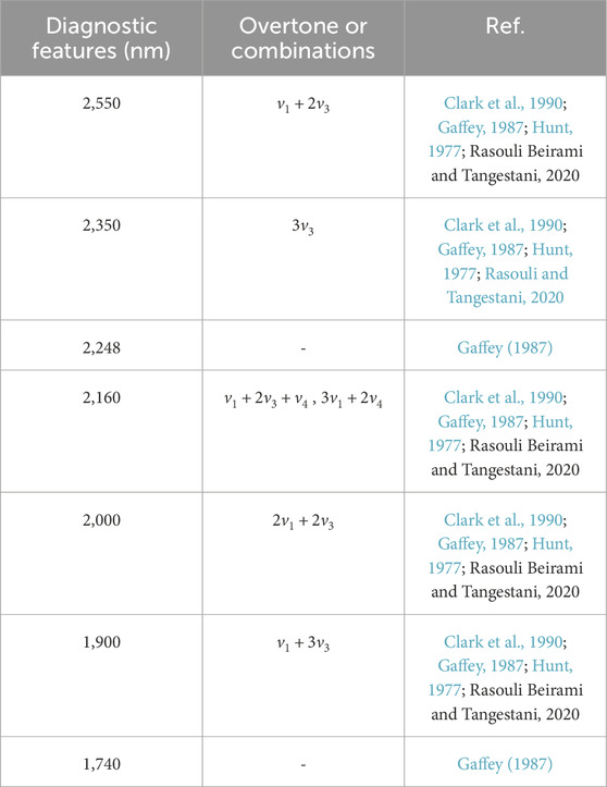
Table 1. Diagnostic bands of carbonate rocks in near-infrared region.
Building on previous research and considering the spectral characteristics of samples from the study area, we employ a boxplot methodology to ascertain the range of feature bands for carbonate rock minerals. The specific steps are outlined below:
(1) Determination of the approximate positions of diagnostic bands. Considering the characteristics of the samples, we determined the approximate positions of the absorption bands specific to dolomite minerals in this region.
(2) Location of absorption valleys. The absorption valleys near the diagnostic bands determined in the preceding step were identified.
(3) Extraction of shoulder bands. The left and right shoulder wavelengths for each absorption valley (λs1 and λs2, respectively) were extracted (see Figure 3).
(4) Definition of interval boundaries. The boundaries of intervals were established via the boxplot analysis of shoulder wavelengths (Tukey, 1977). We establish the first quartile (Q1) of the left shoulder band and the third quartile (Q3) of the right shoulder band as the boundary bands for each interval. Here, Q1 represents the first quartile, indicating that 25% of the data are below this value, and Q3 represents the third quartile, indicating that 75% of the data set are below this threshold. This analytical method is designed to capture prevalent patterns across most samples, effectively minimizing the effect of outliers.
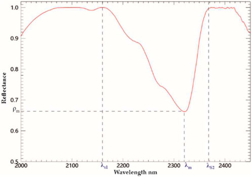
Figure 3. Local waveform features, λm: the wavelength of the absorption valley’s bottom, λs1: left shoulder wavelength, λs2: right shoulder wavelength.
Feature selection based on RFFIM employs an RF algorithm to rank and select input features according to the criteria. In classification tasks, criteria such as Gini impurity or information gain are typically employed, whereas variance reduction is used in regression problems. Since this study involved a regression problem, we chose variance reduction as the evaluation criterion (Breiman, 2001; Verikas et al., 2011). The specific steps were as follows:
(1) Construction of decision trees. Assume a total of p training samples, each with
(2) Contribution of each feature to variance reduction. The contribution of each feature
where
(3) Total contribution to variance reduction. The total contribution to variance reduction
(4) Quantification of feature importance. The importance of feature
SVR is a regression analysis method derived from the principles of SVM. The foundational concept of SVR is to seek an optimal balance between model accuracy and generalizability (Smola and Schölkopf, 2004; Iglesias, 2020). The primary aim of SVR is to identify a smooth model function that minimizes the discrepancy between the estimated and actual values. The linear form of this function is given by Eq. 4:
where
A central aspect of SVR is its focus on a subset of data points known as support vectors, which are determined by the ε-insensitive zone. This zone allows small estimation errors to be ignored while considering only significant deviations in model accuracy. In addition, SVR introduces slack variables
where
In this study, a linear SVR was employed due to the limited number of available samples.
In this study, a MSK-RFFIM-SVR scheme was developed for estimating dolomite content. In this scheme, MSK-RFFIM is used for feature selection in hyperspectral data, while the SVR algorithm is employed for inversion modeling. The workflow of this approach is illustrated in Figure 4, and the specific implementation steps were as follows:
(1) Preprocessing. The hyperspectral data were preprocessed via outlier deletion and continuum removal.
(2) Preliminary feature selection based on the MSK. After analyzing the spectral characteristics of dolomite minerals, box plots were employed to identify the spectral feature regions of the samples, thereby facilitating the preliminary screening of the original hyperspectral bands.
(3) Secondary feature selection based on the RFFIM. An RF algorithm was used to rank the importance of the preliminarily screened features, and the top 50 bands were selected.
(4) Modeling. The top 50 bands selected in the preceding step were used as input variables for the machine learning model to estimate the dolomite content. The results were evaluated to ensure the model’s effectiveness.
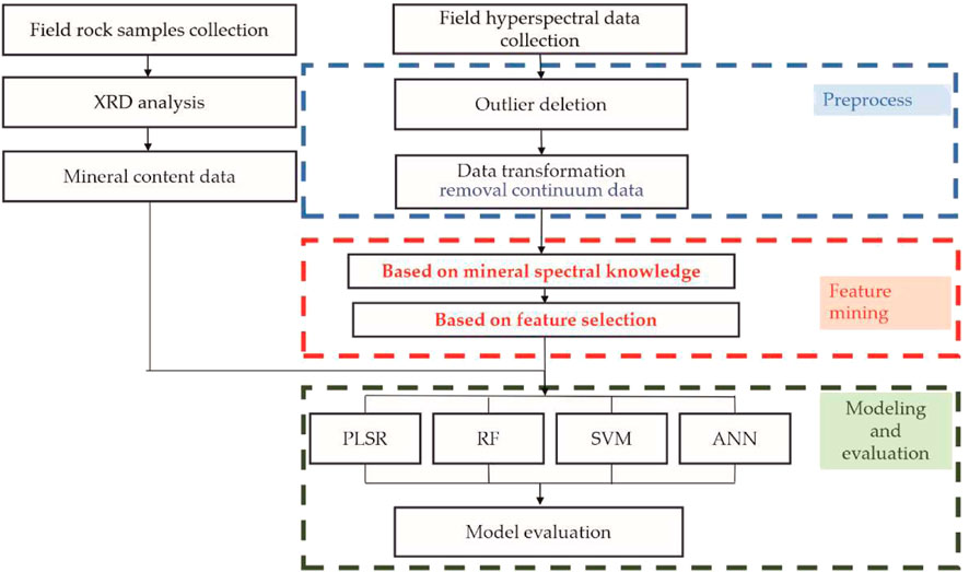
Figure 4. The workflow of dolomite content estimation.
In this study, we have developed the MSK-RFFIM-SVM inversion scheme for estimating dolomite content and verified its effectiveness in comparison to other input variables and modeling methods. The input variables considered in the comparison ranged from Input V1 to Input V8, defined as follows: Input V1 retained all continuum-removed bands; Input V2 selected features based on the MSK; Input V3 utilized the top 50 features selected by RFFIM; Input V4 was based on our MSK-RFFIM method; Input V5 was the top 50 features selected based on correlation coefficients; Input V6 and Input V7 were obtained by transforming hyperspectral data using principal component analysis (PCA) and Kernel PCA (KPCA), respectively, and selecting the top 20 components for each; and Input V8 employs feature selection based on the local waveform characteristics, including the wavelength and reflectance of the bottom of the absorption valley’s, the double-shoulder wavelengths, and the width, height, area, and symmetry of each absorption valley. The detailed extraction methods can be found in Hecker et al. (2019). Table 2 presents detailed information on these eight input variables. The machine learning algorithms included in the comparison were PLSR, RF, SVM and ANN (multilayer perceptron). All algorithms in this experiment were implemented using the Python programming language.
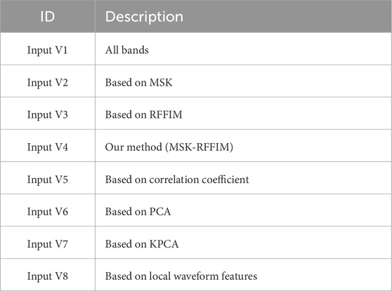
Table 2. Description of eight input variables.
To select the best model hyperparameters, we aimed to minimize the number of hyperparameters requiring tuning, thereby reducing model complexity, and enhancing its generalizability. In this study, the ‘GridSearchCV’ method from the ‘sklearn’ library was employed to determine the optimal hyperparameters of the model. ‘GridSearchCV’ integrates grid search with cross-validation to identify the most accurate parameters within a specified range, traversing all potential combinations. Based on the hyperparameter tuning range presented in Table 3, ‘GridSearchCV’ employed a k-fold cross-validation approach in which the training set was partitioned into k non-overlapping subsets. In each iteration, k−1 subsets were selected for the training set, and the remaining subset served as the validation set for subsequent testing of the trained model. After computing the average score over k iterations, the hyperparameter combination with the highest mean score was selected as the optimal choice. In this study, k was set to 5.
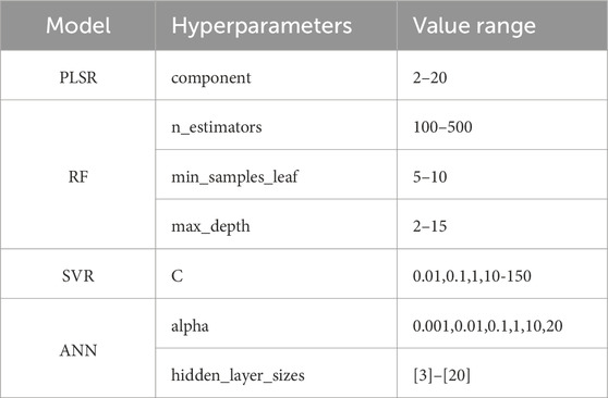
Table 3. Hyperparameters and optimization range.
The evaluation metrics in this study were the coefficient of determination (R2) and root mean square error (RMSE), as shown in Eqs 6, 7:
where
After outlier removal, 203 samples were retained for subsequent work. Based on previous studies, the dolomite mineral exhibits seven significant features in the near-infrared range (see Section 2.2.2). However, based on the spectral range of our instrument, features around 2,500–2,550 nm were not included, and the characteristics near 2,248 and 1740 nm were extremely weak, bordering on negligible. Therefore, we excluded those three features. Consequently, the characteristic spectral features of dolomite minerals in the study area were primarily distributed around 1900, 2000, 2,160, and 2,350 nm (see Figure 5). Subsequently, we located the corresponding absorption valleys at these four wavelengths and extracted the left and right shoulder wavelengths for boxplot analysis. As depicted in Figure 6. The final feature intervals were determined as 1839–1870,1950–2009, 2,110–2,183 and 2,133–2,386 nm with a total of 416 bands.
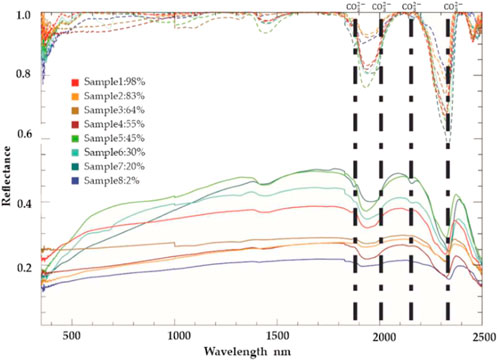
Figure 5. ASD spectrum of carbonate rock samples with different dolomite contents; solid line denotes the original spectrum; dashed line describes the continuum-removed spectrum; black vertical lines represented four diagnostic bands; the percentages in the legend indicate the content of dolomite of samples.

Figure 6. Box diagrams for left and right shoulder wavelengths of four absorption valleys of samples. (A–D) respectively represent the absorption valleys near 1,900 nm, 2,000 nm, 2,160 nm, and 2,350 nm.
In total, 203 samples were used in the modeling process. These samples were randomly divided into a test set and a training set, with 80% (162 samples) designated as training samples and 20% (41 samples) as testing samples.
Table 4 and Figure 7 show the results of the accuracy evaluation for dolomite estimation based on eight features extracted from the continuum-removed data and four machine learning models. In Table 4, our method, along with the optimal and average accuracy values, is highlighted in bold font.
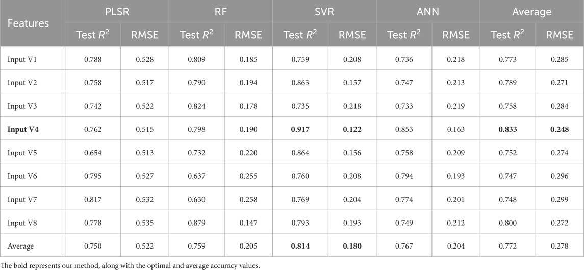
Table 4. Accuracy assessment of dolomite content estimation based on continuum-removal data.
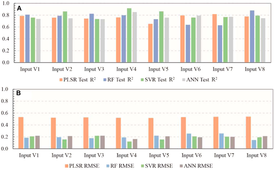
Figure 7. Accuracy assessment of dolomite content estimation based on continuum-removed data, (A): Test R2 assessment (B): RMSE assessment.
First, regarding input variables, significant disparities in performance were observed among the eight input variables across the four machine learning models (Table 4; Figure 7). For the PLSR model, the highest accuracy was achieved when using Input V7, while the lowest accuracy was observed with Input V3. Conversely, for the RF model, the highest and lowest accuracies were, respectively, observed with Input V8 and Input V7. The results obtained using the SVR and ANN models were consistent: Input V4 yielded the highest accuracy, whereas Input V3 resulted in the lowest accuracy. The average test R2and RMSE values were calculated for all input features and are presented in the two rightmost columns of Table 4. The average Test R2values for the eight input variables decreased in the following order: Input V4 > Input V5 > Input V2 > Input V8 > Input V7 > Input V6 > Input V1 > Input V3. The results indicate that Input V4 achieved the best overall performance among all input features.
Next, comparing the different machine learning models, the four models exhibited different performances when combined with different input variables. When selecting Input V1, Input V3, and Input V8, the RF model demonstrated the highest accuracy, while the ANN model had the lowest accuracy. With Input V2, the SVR model displayed the highest accuracy, whereas the ANN model had the lowest. For Input V4 and Input V5, the SVR model achieved the highest accuracy, and the PLSR model result in the lowest accuracy. With Input V6 and Input V7, the PLSR model achieved the highest accuracy, while RF results in the lowest. Although the test R2 value of PLSR was not always the lowest among the four models, its RMSE value was significantly higher than those of the other three models, as shown in Figures 7A, B, indicating that PLSR was not suitable for estimating dolomite mineral content in this study. Furthermore, the average test R2 value for all input variables was calculated across the four models (see Table 4), resulting in the following order in average test R2 accuracy: SVR > ANN > RF > PLSR. The results suggest that among the tested models, SVR achieved best average accuracy and thus the best overall performance.
In summary, by combining the good feature selection performance of MSK-RFFIM with the overall accuracy of SVR, the integrated MSK-RFFIM-SVR model demonstrated exceptional efficacy for estimating the dolomite content in carbonate rocks. Figure 8 shows a detailed comparison of the estimation accuracies for each input variable when integrated with the SVR model. The MSK-RFFIM-SVR approach proposed in this study achieved a test R2 of 0.917 and an RMSE of just 0.122, superior to other methods.
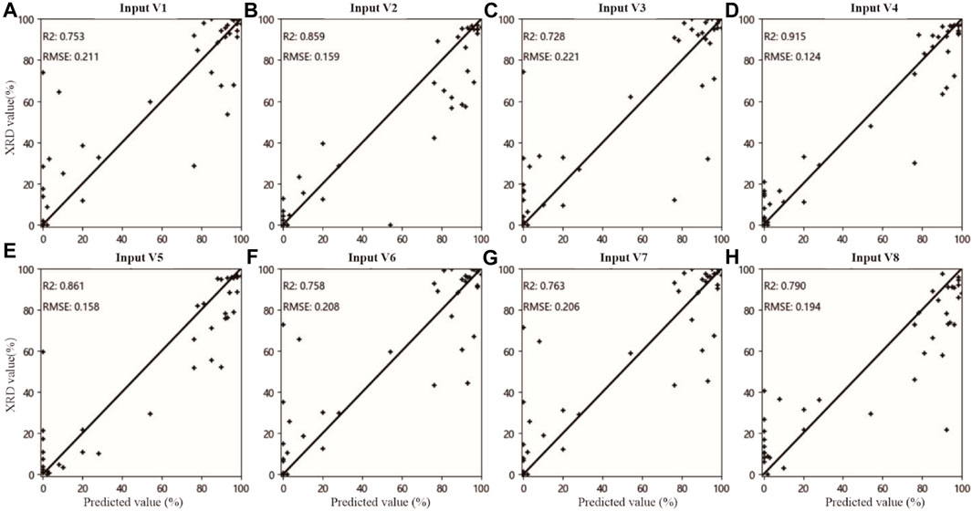
Figure 8. Comparison of the estimated results of all input variables based on continuum-removed data and SVM algorithm with the XRD data of the test samples, (A–H) corresponds to Input V1- Input V8 respectively.
The purpose of continuum removal is to enhance information while simultaneously eliminating background noise. A correlation analysis was conducted to compare the dolomite content based on both the original and continuum-removed hyperspectral data (Figure 9). As shown in Figure 9A, the original hyperspectral data was influenced by environmental factors and background noise and showed relatively low variance in reflectance. Consequently, the correlation coefficients between the reflectance of all bands and the dolomite content were relatively uniform. However, the correlations between continuum-removed data and the dolomite content exhibited more pronounced variations (Figure 9B). Therefore, continuum removal improved the quality of the hyperspectral data and facilitated subsequent feature selection and modeling.
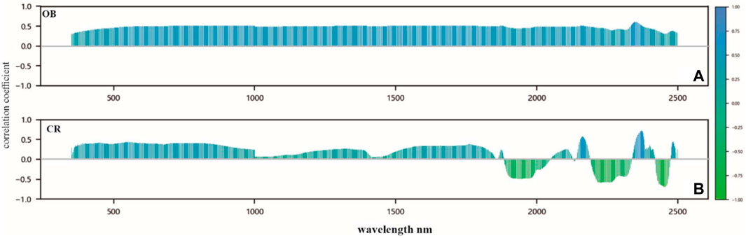
Figure 9. (A,B) are correlation analysis of original data and continuum-removed data with the dolomite content respectively, OB: original hyperspectral data, CR: continuum-removed data.
The hybrid MSK-RFFIM feature selection method proposed in this paper leverage the strengths of both constituent methods. As shown in Table 4, the MSK-RFFIM method resulted in enhanced accuracy compared with either the MSK or RFFIM method alone. Previous studies have also indicated that hybrid feature selection methods can enhance the overall effectiveness of feature selection (Chen et al., 2023; Wang et al., 2023). The MSK-RFFIM method was further analyzed using the top 20 bands from Input V3, Input V4, and Input V5 (refer to Table 5). Some selected bands of InputV3 were situated below 1800 nm; the reflectance of these bands is likely related to the water molecules present within the minerals. Similarly, for Input V5, a significant number of the first 20 features included bands above 2,400 nm. Given that the detection limit of the employed equipment was 2,500 nm, the reflectance spectra in the proximal wavelength range (2,450–2,500 nm) tend to exhibit a sawtooth pattern, suggesting that they may be unreliable due to noise or intrinsic equipment limitations. Therefore, using the MSK method as a preliminary screening tool effectively eliminated irrelevant features, thereby reducing interference in subsequent models. Further comparison between the MSK and MSK-RFFIM appoaches (as seen in Table 4; Figure 8, Input V2 and Input V4) indicated a notable improvement in the average test R2 for MSK-RFFIM (0.833 compared with 0.789 for MSK). This improvement is likely attributed to the ability of the RF algorithm to eliminate unimportant features and reduce the effect of redundant features (Genuer, 2010).
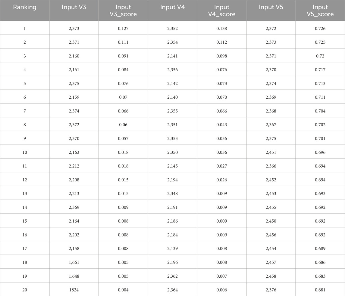
Table 5. The Top 20 features of input variables and their ranking index scores.
In addition to accuracy, we also considered the sensitivity of the model hyperparameters. High sensitivity to model hyperparameters complicates the tuning of machine learning algorithms; minor adjustments can markedly affect outcomes, potentially undermining the generalization ability of the model. Here, we conducted a sensitivity analysis of model hyperparameters based on the optimal approach. The hyperparameter sensitivity of the model was evaluated based in terms of the estimation accuracy of different hyperparameter combinations with the four machine learning algorithms.
In Figure 10, the vertical axis represents the ‘mean_test_score’ while the horizontal axis represents the different hyperparameter combinations for each machine learning algorithm. The ‘mean_test_score’ represents the average accuracy from a 5-fold cross-validation on training samples using the ‘GridSearchCV’ algorithm. For PLSR and SVM, optimization focused on a single hyperparameter: ‘n_components’ for PLSR and ‘C′ for SVM (Figures 10A, C). By contrast, RF and ANN required adjustments across multiple hyperparameters; the hyperparameter tuning ranges for each are detailed in Table 3. Consequently, RF and ANN possessed a total of 84 hyperparameter combinations, which form the horizontal axis (Figures 10B, D). Figure 10 illustrates that both the PLSR and RF models exhibited minimal sensitivity to hyperparameter variations. The SVM model showed unstable performance when the ‘C′ value was low, but stabilized when the ‘C′ hyperparameter reached a certain critical value (Wang et al., 2019). Conversely, the ANN model exhibited the highest sensitivity to the hyperparameters, consistent with previous finding (Rodriguez-Galiano et al., 2015).
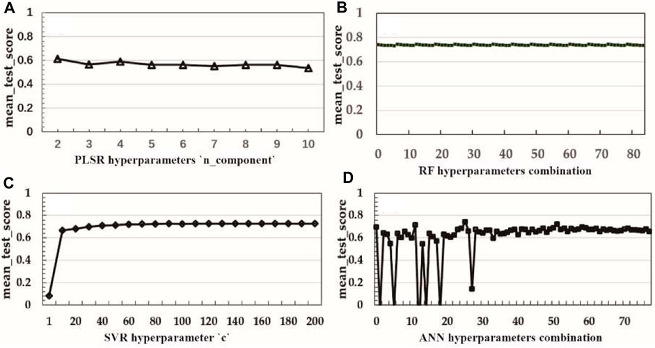
Figure 10. Sensitivity analysis of model hyperparameters. (A–D) represent the effects of hyperparameter variations in PLSR, RF, SVR, and ANN on accuracy.
In summary, PLSR was not favorable due to its significant error. The RF model stood out for its stability and simplicity in parameter tuning. However, the accuracy of the RF model was lower compared with other non-linear models. The ANN algorithm achieved higher accuracy, but demonstrated notable sensitivity to the model parameters, complicating hyperparameter optimization. Overall, the SVR model achieved the optimal balance among accuracy, parameter count, and parameter sensitivity. It mainly optimizes the ‘C′ parameter, with performance plateauing beyond a certain threshold. Therefore, the experimental results suggest that the SVR algorithm is the optimal choice.
The primary focus of this study was carbonate rocks, other rock types were not considered. Furthermore, during hyperspectral sampling, sampling points with relatively fresh surfaces were specifically chosen, while severely weathered areas intentionally avoiding to prevent the known effect of weathering on spectral data (Shin et al., 2019). Future work will involve samples taken from weathered surfaces and comparative analysis of the accuracy of different features and modeling algorithms between weathered and fresh surfaces.
This paper presents the MSK-RFFIM-SVR scheme for estimating mineral content based on field-collected hyperspectral data. In this scheme, following the preprocessing of the hyperspectral data, a hybrid MSK-RFFIM approach is used for feature selection. The SVR algorithm is then used to inversely estimate the dolomite content. Compared with conventional machine learning methods, this scheme more effectively selects key features of the target mineral, significantly enhancing model accuracy. Our estimation results for dolomite samples produced a test R2 value of 0.91 and an RMSE of 0.122. The proposed approach is especially advantageous for field outcrop exploration and can provide high-precision quantitative data to support field geologists in identifying distribution of outcrop minerals, understanding the reservoir characteristics, and detecting changes in ancient environments. The carbonate rock samples in this study mainly consisted of dolomite and calcite. Future research will explore more complex mineral compositions and surface environmental conditions in carbonate rock outcrops.
The raw data supporting the conclusion of this article will be made available by the authors, without undue reservation.
WW: Investigation, Methodology, Validation, Writing–original draft, Writing–review and editing. YS: Conceptualization, Investigation, Validation, Writing–review and editing. ZH: Methodology, Writing–review and editing. QW: Writing–review and editing. FD: Writing–review and editing. YH: Data curation, Writing–review and editing. KZ: Data curation, Writing–review and editing.
The author(s) declare that financial support was received for the research, authorship, and/or publication of this article. This research was funded by CNPC (China National Petroleum Corporation) Technology Project., grant number 2021DJ0402.
Thanks to the Research Institute of Petroleum Exploration and Development, CNPC for providing the funding for this project. Special appreciation to Qihong Zeng, Youyan Zhang and Zhiguo Ma from the Research Institute of Petroleum Exploration and Development, CNPC for their assistance in this project.
The authors declare that the research was conducted in the absence of any commercial or financial relationships that could be construed as a potential conflict of interest.
The authors declare that this study received funding from CNPC. The funder had the following involvement in the study: study design, data collection and analysis, decision to publish, and preparation of the manuscript.
All claims expressed in this article are solely those of the authors and do not necessarily represent those of their affiliated organizations, or those of the publisher, the editors and the reviewers. Any product that may be evaluated in this article, or claim that may be made by its manufacturer, is not guaranteed or endorsed by the publisher.
Asadzadeh, S., and Souza Filho, C. R. (2016). A review on spectral processing methods for geological remote sensing. Int. J. Appl. Earth Observation Geoinformation 47, 69–90. doi:10.1016/j.jag.2015.12.004
Baugh, W. M., Kruse, F. A., and Atkinson, W. W. (1998). Quantitative geochemical mapping of ammonium minerals in the Southern Cedar Mountains, Nevada, using the airborne visible/infrared imaging spectrometer (AVIRIS). Remote Sens. Environ. 65 (3), 292–308. doi:10.1016/S0034-4257(98)00039-X
Bennett, K. P., and Mangasarian, O. L. (1992). Robust linear programming discrimination of two linearly inseparable sets. Optimization methods and software 1 (1), 23–24. doi:10.1080/10556789208805504
Carranza, E. J. M., and Laborte, A. G. (2015). Random forest predictive modeling of mineral prospectivity with small number of prospects and data with missing values in Abra (Philippines). Comput. Geosciences 74 (10), 60–70. doi:10.1016/j.cageo.2014.10.004
Chatterjee, S., Mastalerz, M., Drobniak, A., and Karacan, C. Ö. (2022). Machine learning and data augmentation approach for identification of rare earth element potential in Indiana Coals, USA. Int. J. Coal Geol. 259, 104054. doi:10.1016/j.coal.2022.104054
Chen, L., Sui, X., Liu, R., Chen, H., Li, Y., Zhang, X., et al. (2023). Mapping alteration minerals using ZY-1 02D hyperspectral remote sensing data in coalbed methane enrichment areas. Remote Sens. 15 (14), 3590. doi:10.3390/rs15143590
Clark, R. N., King, T. V., Klejwa, M., Swayze, G. A., and Vergo, N. (1990). High spectral resolution reflectance spectroscopy of minerals. J. Geophys. Res. 95 (B8), 12653–12680. doi:10.1029/JB095iB08p12653
Clark, R. N., and Roush, T. L. (1984). Reflectance spectroscopy: quantitative analysis techniques for remote sensing applications. J. Geophys. Res. Solid Earth 89 (B7), 6329–6340. doi:10.1029/JB089iB07p06329
Dawson, H. L., Dubrule, O., and John, C. M. (2023). Impact of dataset size and convolutional neural network architecture on transfer learning for carbonate rock classification. Comput. Geosciences 171, 105284. doi:10.1016/j.cageo.2022.105284
Deepa, C., Shetty, A., and Narasimhadhan, A. V. (2023). Performance evaluation of dimensionality reduction techniques on hyperspectral data for mineral exploration. Earth Sci. Inf. 16 (1), 25–36. doi:10.1007/s12145-023-00956-2
Gaffey, S. J. (1987). Spectral reflectance of carbonate minerals in the visible and near infrared (0.35–2.55 um): Anhydrous carbonate minerals. J. Geophys. Res. 92 (B2), 1429–1440. doi:10.1029/JB092iB02p01429
Genuer, R., Poggi, J. M., and Tuleau-Malot, C. (2010). Variable selection using random forests. Pattern Recognit. Lett. 31 (3), 2225–2236. doi:10.1016/j.patrec.2010.03.014
Haest, M., Cudahy, T., Laukamp, C., and Gregory, S. (2012). Quantitative mineralogy from infrared spectroscopic data. I. Validation of mineral abundance and composition scripts at the Rocklea Channel iron deposit in western Australia. Econ. Geol. 107 (2), 209–228. doi:10.2113/econgeo.107.2.209
Hamedianfar, A., Laakso, K., Middleton, M., Törmänen, T., Köykkä, J., and Torppa, J. (2023). Leveraging high-resolution long-wave infrared hyperspectral laboratory imaging data for mineral identification using machine learning methods. Remote Sens. 15 (19), 4806. doi:10.3390/rs15194806
He, Y., Zhou, Y., Wen, T., Zhang, S., Huang, F., Zou, X., et al. (2022). A review of machine learning in geochemistry and cosmochemistry: method improvements and applications. Appl. Geochem. 140, 105273. doi:10.1016/j.apgeochem.2022.105273
Hebert, B., Baron, F., Robin, V., Lelievre, K., Dacheux, N., Szenknect, S., et al. (2019). Quantification of coffinite (USiO4) in roll-front uranium deposits using visible to near infrared (Vis-NIR) portable field spectroscopy. J. Geochem. Explor. 199, 53–59. doi:10.1016/j.gexplo.2019.01.003
Hecker, C., van Ruitenbeek, F. J., van der Werff, H. M., Bakker, W. H., Hewson, R. D., and van der Meer, F. D. (2019). Spectral absorption feature analysis for finding ore: a tutorial on using the method in geological remote sensing. IEEE Geoscience Remote Sens. Mag. 7 (2), 51–71. doi:10.1109/MGRS.2019.2899193
Hunt, G. R. (1977). Spectral signatures of particulate minerals in the visible and near infrared. Geophysics 42 (3), 501–513. doi:10.1190/1.1440721
Iglesias, C., Antunes, I., Albuquerque, M., Martínez, J., and Taboada, J. (2020). Predicting ore content throughout a machine learning procedure – an Sn-W enrichment case study. J. Geochem. Explor. 208, 106405. doi:10.1016/j.gexplo.2019.106405
Jia, X., Kuo, B. C., and Crawford, M. M. (2013). Feature mining for hyperspectral image classification. Proc. IEEE 101 (3), 676–697. doi:10.1109/JPROC.2012.2229082
Knox, N. M., Grunwald, S., McDowell, M. L., Bruland, G. L., Myers, D. B., and Harris, W. G. (2015). Modelling soil carbon fractions with visible near-infrared (VNIR) and mid-infrared (MIR) spectroscopy. Geoderma 239–240, 229–239. doi:10.1016/j.geoderma.2014.10.019
Kumar, V. (2014). Feature selection: a literature review. Smart Comput. Rev. 4 (3), 211–229. doi:10.6029/smartcr.2014.03.007
Kurz, T. H., Buckley, S. J., and Howell, J. A. (2012). Close-range hyperspectral imaging for geological field Studies: workflow and methods. Int. J. Remote Sens. 34 (5), 1798–1822. doi:10.1080/01431161.2012.727039
Kurz, T. H., Miguel, G. S., Dubucq, D., Kenter, J., Miegebielle, V., and Buckley, S. J. (2022). Quantitative mapping of dolomitization using close-range hyperspectral imaging: kimmeridgian carbonate ramp, Alacón, NE Spain. Geosphere 18 (2), 780–799. doi:10.1130/GES02312.1
Lin, N., Liu, H., Li, G., Wu, M., Li, D., Jiang, R., et al. (2022). Extraction of mineralized indicator minerals using ensemble learning model optimized by SSA based on hyperspectral image. Open Geosci. 14 (1), 1444–1465. doi:10.1515/geo-2022-0436
Okyay, Ü., Khan, S., Lakshmikantha, M., and Sarmiento, S. (2016). Ground-based hyperspectral image analysis of the lower Mississippian (Osagean) Reeds Spring Formation rocks in southwestern Missouri. Remote Sens. 8 (12), 1018. doi:10.3390/rs8121018
Rasouli, B. M., and Tangestani, M. H. (2020). A new band ratio approach for discriminating calcite and dolomite by ASTER imagery in arid and semiarid regions. Natural Resources Research 29 (5), 2949–2965. doi:10.1007/s11053-020-09648-w
Rasti, B., Hong, D., Hang, R., Ghamisi, P., Kang, X., Chanussot, J., et al. (2020). Feature extraction for hyperspectral imagery: the evolution from shallow to deep: overview and toolbox. IEEE Geoscience Remote Sens. Mag. 8 (4), 60–88. doi:10.1109/MGRS.2020.2979764
Rodriguez-Galiano, V., Sanchez-Castillo, M., Chica-Olmo, M., and Chica-Rivas, M. J. O. G. R. (2015). Machine learning predictive models for mineral prospectivity: an evaluation of neural networks, random forest, regression trees and support vector machines. Ore Geol. Rev. 71, 804–818. doi:10.1016/j.oregeorev.2015.01.001
Rodriguez-Galiano, V. F., Luque-Espinar, J. A., Chica-Olmo, M., and Mendes, M. P. (2018). Feature selection approaches for predictive modelling of groundwater nitrate pollution: an evaluation of filters, embedded and wrapper methods. Sci. Total Environ. 624, 661–672. doi:10.1016/j.scitotenv.2017.12.152
Saikia, P., Baruah, R. D., Singh, S. K., and Chaudhuri, P. K. (2020). Artificial neural networks in the domain of reservoir characterization: a review from shallow to deep models. Comput. Geosciences 135, 104357. doi:10.1016/j.cageo.2019.104357
Seo, J., Yu, J., and Wang, L. (2023). Indicator spectral bands and logistic models for detecting diesel and gasoline polluted soils based on close-range hyperspectral image data. IEEE Trans. Geoscience Remote Sens. 61, 1–13. doi:10.1109/TGRS.2023.3264967
Shin, J. H., Yu, J., Wang, L., Kim, J., Koh, S. M., and Kim, S. O. (2019). Spectral responses of heavy metal contaminated soils in the vicinity of a hydrothermal ore deposit: a case study of Boksu Mine, South Korea. IEEE Trans. Geoscience Remote Sens. 57 (6), 4092–4106. doi:10.1109/TGRS.2018.2889748
Shirmard, H., Farahbakhsh, E., Muller, R. D., and Chandra, R. (2022). A review of machine learning in processing remote sensing data for mineral exploration. Remote Sens. Environ. 268, 112750. doi:10.1016/j.rse.2021.112750
Sim, J., Dixit, Y., Mcgoverin, C., Oey, I., Frew, R., Reis, M. M., et al. (2023). Support vector regression for prediction of stable isotopes and trace elements using hyperspectral imaging on coffee for origin verification. Food Res. Int. 174, 113518. doi:10.1016/j.foodres.2023.113518
Smola, A. J., and Schölkopf, B. (2004). A tutorial on support vector regression. Statistics Comput. 14 (3), 199–222. doi:10.1023/B:STCO.0000035301.49549.88
Tan, K., Chen, L., Wang, H., Liu, Z., Ding, J., and Wang, X. (2023). Estimation of the distribution patterns of heavy metal in soil from airborne hyperspectral imagery based on spectral absorption characteristics. J. Environ. Manag. 347, 119196. doi:10.1016/j.jenvman.2023.119196
Tan, K., Wang, H., Chen, L., Du, Q., Du, P., and Pan, C. (2020). Estimation of the spatial distribution of heavy metal in agricultural soils using airborne hyperspectral imaging and random forest. J. Hazard. Mater. 382, 120987. doi:10.1016/j.jhazmat.2019.120987
Thomas, R. N., and Gupta, R. (2020). “Feature selection techniques and its importance in machine learning: a survey,” in 2020 IEEE International Students’ Conference on Electrical, Electronics and Computer Science (SCEECS), Bhopal, India, 22-23 February 2020 (IEEE), 1–6.
van der Meer, F. D., van der Werff, H. M., van Ruitenbeek, F. J., Hecker, C. A., Bakker, W. H., Noomen, M. F., et al. (2012). Multi- and hyperspectral geologic remote sensing: a review. Int. J. Appl. Earth Observation Geoinformation 14 (1), 112–128. doi:10.1016/j.jag.2011.08.002
Verikas, A., Gelzinis, A., and Bacauskiene, M. (2011). Mining data with random forests: a survey and results of new tests. Pattern Recognit. 44 (2), 330–349. doi:10.1016/j.patcog.2010.08.011
Wang, S., Chen, Y., Wang, M., and Li, J. (2019). Performance comparison of machine learning algorithms for estimating the soil salinity of salt-affected soil using field spectral data. Remote Sens. 11 (22), 2605. doi:10.3390/rs11222605
Wang, Y., Niu, R., Hao, M., Lin, G., Xiao, Y., Zhang, H., et al. (2023). A method for heavy metal estimation in mining regions based on SMA-PCC-RF and reflectance spectroscopy. Ecol. Indic. 154, 110476. doi:10.1016/j.ecolind.2023.110476
Zaini, N., van der Meer, F., and van der Werff, H. (2014). Determination of carbonate rock chemistry using laboratory-based hyperspectral imagery. Remote Sens. 6 (5), 4149–4172. doi:10.3390/rs6054149
Zhang, T., Fu, Q., Tian, R., Zhang, Y., and Sun, Z. (2023a). A spectrum contextual self-attention deep learning network for hyperspectral inversion of soil metals. Ecol. Indic. 152, 110351. doi:10.1016/j.ecolind.2023.110351
Zhang, Y., Wei, L., Lu, Q., Zhong, Y., Yuan, Z., Wang, Z., et al. (2023b). Mapping soil available copper content in the mine tailings pond with combined simulated annealing deep neural network and UAV hyperspectral images. Environ. Pollut. 320, 120962. doi:10.1016/j.envpol.2022.120962
Zhou, M., Zou, B., Tu, Y., Feng, H., He, C., Ma, X., et al. (2022). Spectral response feature bands extracted from near standard soil samples for estimating soil Pb in a mining area. Geocarto Int. 37 (26), 13248–13267. doi:10.1080/10106049.2022.2076921
Keywords: hyperspectral, dolomite content, hybrid feature selection, machine learning, outcrop
Citation: Wei W, Shao Y, Hu Z, Wang Q, Deng F, Huang Y and Zhao K (2024) Estimation of the dolomite content of carbonate rock outcrops based on spectral knowledge and machine learning. Front. Earth Sci. 12:1401026. doi: 10.3389/feart.2024.1401026
Received: 14 March 2024; Accepted: 17 May 2024;
Published: 11 June 2024.
Edited by:
Wenguang Wang, Northeast Petroleum University, ChinaReviewed by:
Wang Lihui, Chinese Academy of Sciences (CAS), ChinaCopyright © 2024 Wei, Shao, Hu, Wang, Deng, Huang and Zhao. This is an open-access article distributed under the terms of the Creative Commons Attribution License (CC BY). The use, distribution or reproduction in other forums is permitted, provided the original author(s) and the copyright owner(s) are credited and that the original publication in this journal is cited, in accordance with accepted academic practice. No use, distribution or reproduction is permitted which does not comply with these terms.
*Correspondence: Yanlin Shao, NTAwMTcxQHlhbmd0emV1LmVkdS5jbg==
Disclaimer: All claims expressed in this article are solely those of the authors and do not necessarily represent those of their affiliated organizations, or those of the publisher, the editors and the reviewers. Any product that may be evaluated in this article or claim that may be made by its manufacturer is not guaranteed or endorsed by the publisher.
Research integrity at Frontiers
Learn more about the work of our research integrity team to safeguard the quality of each article we publish.