 Octavio Fashé-Raymundo1
 José Luis Flores-Rojas2*
 René Estevan-Arredondo2
 Lucy Giráldez-Solano2
 Luis Suárez-Salas2Elias Sanabria-Pérez3
 Hugo Abi Karam4Yamina Silva2
- 1Universidad Nacional Mayor de San Marcos, Lima, Peru
- 2Instituto Geofísico del Perú, Lima, Peru
- 3Universidad Nacional del Centro del Perú, Facultad de Ingeniería Química, Huancayo, Peru
- 4Universidade Federal de Rio de Janeiro, Rio de Janeiro - Universidade Federal de Rio de Janeiro/Instituto de Geociências/Centro de Ciências Matemáticas e da Natureza, Rio de Janeiro, Brazil
The present study aims to comprehensively assess the solar irradiance patterns in the western zone of the Mantaro Valley, a region of ecological and agricultural significance in the central Peruvian Andes. Leveraging radiation data from the Baseline surface Radiation Network (BSRN) sensors located in the Huancayo Geophysical Observatory (HYGO-12.04°S,75.32°W, 3350 masl) spanning from 2017 to 2022, the research delves into the seasonal variations and trends in surface solar irradiance components. Actually, the study investigates the diurnal and seasonal variations of solar irradiance components, namely diffuse (EDF), direct (EDR), and global (EG) irradiance. Results demonstrate distinct peaks and declines across seasons, with EDR and EDF exhibiting opposing seasonal trends, influencing the overall variability in, EG. Peaks of, EG occurred in spring (3.32 MJ m−2 h−1 at noon), particularly during October (24.14 MJ m-2 day-1), probably associated with biomass-burning periods and heightened aerosol optical depth (AOD). These findings highlight the impact of biomass-burning aerosols on solar radiation dynamics in the region. In general, the seasonal variability of, EG on the HYGO is lower than that observed in other regions of South America at higher latitudes and reach its maximums during spring months. Moreover, the research evaluates various irradiation models to establish correlations between sunshine hours, measured with a solid glass sphere heliograph, and, EG and EDF at different time scales, showing acceptable accuracy to predict. In addition, the sigmoid logistic function emerges as the most effective in correlating the hourly diffuse fraction
1 Introduction
Solar radiation serves as the primary energy source driving surface-atmosphere interactions, influencing a wide array of physical, chemical, and biological processes within Earth’s atmospheric and oceanic systems (Munner, 2004a; Arya, 2005). Understanding the components of solar radiation, namely global
Since 1990, global organizations have emphasized the environmental risks posed by fossil fuels, promoting renewable energy. However, global energy demand is projected to rise by over 50% by 2030 (Sayigh, 2020). In recent decades, there has been a notable surge in investment and development of alternative technologies aimed at producing clean energy from renewable sources. These technologies offer lower environmental impacts compared to traditional ones, garnering significant attention worldwide (Ellabban et al., 2014). The “Renewable Energy Policy Network for the 21st Century Report” highlights a growing interest in renewable energies, with a global push towards achieving net-zero emissions by 2050 (REN21, 2023). Currently, solar and wind power are among the most promising and feasible renewable resources. The implementation of photovoltaic systems
In this context, observations of solar radiation are commonly focused on global radiation. However, many applications require data on irradiation on sloping surfaces. Therefore, it is often necessary to divide global radiation into its beam and diffuse components to derive the specific data needed from the available global radiation measurements. A number of diffuse fraction models are available for averaging times ranging from 1 month to 1 hour or even less. Different diffuse fraction models generally require varying input data. The model proposed by Erbs et al. (1982) only needs the hourly clearness index. The models of Maxwell (1987) and Skartveit and Olseth (1987) require both the hourly clearness index and solar elevation and the model of Skartveit et al. (1998) which added hour-to-hour variability index and regional surface albedo.
Furthermore, the model by Perez et al. (1992) further includes ambient dew-point temperature and an hour-to-hour variability index. From a large multiclimatic database, they derived a computationally efficient model using a four-dimensional look-up table consisting of a
In general, South America lacks sufficient radiometric stations equipped to measure various components of solar radiation, typically only measuring global radiation
Moreover, compared to 1980, projections indicate a decrease in ultraviolet UV-B irradiance by 5%–20% at mid to high latitudes by the end of the 21st century, while a slight increase of 2%–3% is expected in low latitudes. The tropics (25
Particularly, UV solar irradiance measurements were conducted by Suárez Salas et al. (2017) in the Peruvian central Andes, at the HYGO, between January 2003 and December 2006, using a GUV-511 multi-channel filter radiometer. Data analysis revealed daily, monthly, and annual cycles of UV solar irradiance at four wavelengths (305, 320, 340, and 380 nm). Clear sky and all sky conditions were distinguished, with February showing peak values. The highest hourly mean UV Index at noon reached 18.8 under clear sky conditions and 15.5 under all sky conditions, with outlier peaks close to 28. Cloud cover increased spectral irradiance at 340 nm by up to 20%, indicating exceptionally high levels of UV radiation in the tropical central Andes. However, to date, there are no studies aimed at studying solar radiation in the central Peruvian Andes with high quality data.
On the other hand, in Brazil, several studies have investigated solar radiation patterns for different sites using high quality radiometric sensors like BSRN stations (Driemel et al., 2018). For instance, Oliveira et al. (2002b) examines seasonal variations in
The present study aims to comprehensively analyze solar irradiance patterns in the western Mantaro Valley, utilizing data from BSRN sensors at the Huancayo Geophysical Observatory (HYGO), spanning 2017 to 2022, the research investigates seasonal variations and trends in surface solar irradiance components. Specifically, the study explores diurnal and seasonal fluctuations of diffuse
2 Site and location
The measurements in this study were conducted at the Huancayo Geophysical Observatory (HYGO), situated at coordinates 12.04
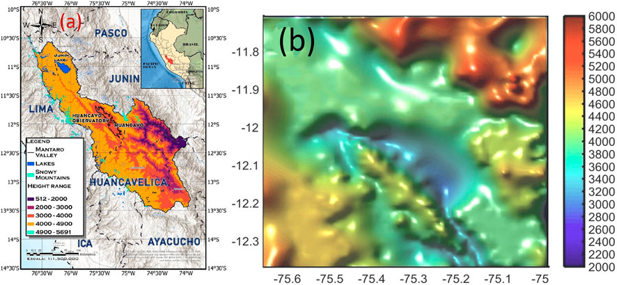
Figure 1. (A) The location of the HYGO (12.05
The climatological data spanning 48 years (1965–2013) from HYGO reveals a predominant unimodal seasonal pattern in precipitation. This pattern distinctly delineates a dry season extending from April to August, followed by a rainy season spanning from September to March. Notably, the latter part of August may witness intense rainfall events, with precipitation steadily increasing until it reaches its zenith during the austral summer, specifically in January through March, as substantiated by prior studies (Silva et al., 2008; Espinoza-Villar et al., 2009). Following this period, a noteworthy decline in precipitation is observed in April. Consequently, approximately 83% of the annual accumulated rainfall occurs during the rainy season, as documented in earlier research (Silva et al., 2010).
Moreover, Flores-Rojas et al. (2019a) shows that the components of the energy budget exhibit both seasonal and daily variations, with the partitioning of net irradiance
During the fall and winter months, the mean monthly
3 Instrumentation
3.1 Sensors
The Geophysical Institute of Peru implemented the Laboratory of Physics, Microphysics and Radiation (LAMAR) in 2015 at the HYGO. LAMAR has a set of varied instruments and sensors that can be used to measure several atmospheric properties with high temporal and spatial resolutions and to validate numerical physical models in the Mantaro valley. All devices were installed in a 6-m high tower as a part of BSRN stations (Figure 2A). The set of radiation sensors contains a set of three pyranometers CMP10 (Kipp & Zonen), a pyrheliometer CHP1 (Kipp & Zonen) and two pyrgeometers CGR4 (Kipp & Zonen) (Figure 2B), to measure the hemispherical shortwave (SW) irradiance components and longwave (LW) irradiance incident and emitted by the surface, respectively. Two of the pyranometers were used to measure the SW global and diffuse irradiances incident at the surface, and the last one was used to measured the SW irradiance reflected by the surface. To measure the diffuse irradiance from the sky by blocking the direct solar irradiance we used a small black sphere mounted on an articulated, shading assembly in a two-axis automatic sun tracker 2AP (Kipp & Zonen). More details about these radiative sensors can be found in recent contributions (Flores-Rojas et al., 2019a; lores-Rojas et al., 2021). Figure 2C shows the heliograph from Campbell-Stokes installed at 1.5 m on the HYGO to measure sunshine hours and finally, Figure 2D, shows the location of LAMAR’s instruments and sensors inside the HYGO.
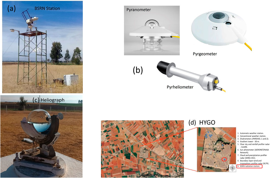
Figure 2. (A) BSRN radiation tower of 6 m high with radiative sensors located in the HYGO. (B) Pyranometer, pyrgeometer and pyrheliometer installed in the BSRN station. (C) Heliograph from Campbell-Stokes installed at 1.5 m in HYGO. (D) Agricultural area around the HYGO and the location of the set of instruments inside the HYGO. The location of the BSRN station is highlighted in red box.
4 Methodology
4.1 Database
In this study, we evaluate the primary atmospheric variables on the HYGO by analyzing measurements collected from a set of automatic sensors belonging to the surface weather station as illustrated in Figure 2D and the solar irradiance data by analyzing measurements from the BSRN station showed in Figures 2A, B. Both systems are operated by the Geophysical Institute of Peru (IGP). The details of these data sources are provided below:
1. Values of air temperature (
2. Values of global, diffuse and direct solar irradiance (W
In meteorological measurement systems, the recording of data often encounters challenges. In the case of radiometers, measurement errors typically arise from several factors, including sensor misalignment or tilting, interference from nearby objects causing shadowing and reflections, and the accumulation of dust and moisture on the sensor dome (Bacher et al., 2013; Vuilleumier et al., 2014). Additionally, the behavior of solar radiation components is influenced by various factors such as cloudiness patterns, aerosol optical depth, surface albedo, cloud type, among others (Perez et al., 1990; Gueymard, 2005), making the development of universal models a complex task. For this work, we conducted distinct data quality checks to identify and rectify missing data, data points that clearly deviated from physical constraints, and extreme data outliers.
In cases where data were confirmed as ‘erroneous’ or ‘missing,’ the corresponding data fields were filled with a specific key sequence of numbers unique to the reporting location, serving as a clear indicator of the problematic observations. Any data associated with flagged ‘bad’ or ‘missing’ data was subsequently excluded from the dataset. Furthermore, a secondary filter was applied to eliminate hours featuring observations that violated fundamental physical principles or conservation laws. This included the removal of hours where reported values exhibited anomalies such as negative radiation values, diffuse fractions exceeding 1, beam radiation surpassing extraterrestrial beam radiation levels, and instances where the dew point temperature exceeded the dry bulb temperature (Reindl et al., 1990).
Additionally, we conducted a rigorous visual quality control process on the dataset, aiming to identify and rectify inconsistencies and spikes that could be attributed to electronic malfunctions within the data acquisition system. Furthermore, we applied the methodology introduced by Younes et al. (2005) and Journee and Cedric (2010) to analyze the time series data. Data points were considered valid if they met specific criteria, including a solar elevation angle
Here,
However, the most stringent criterion,
Following rigorous data quality control procedures, we identified and selected data equivalent to 1850 days (44 400 h) to effectively capture the seasonal variations in solar irradiance across the region. This dataset encompasses approximately 88% of the entire observational period. Subsequently, comprehensive statistical analyses were conducted on various measurements, including those of
The present study employs two key indexes to analyze atmospheric radiometric properties and develop empirical and correlation models: the clearness index
4.2 Solar irradiance models
To develop the regression models of this section, the filtered dataset from May 2017 to December 2022 (1850 days or 44 400 h) as described in Section 4.1 was divided into two segments. Sixty percent (60%) of the total filtered dataset chosen randomly (1,110 days or 26 640 h), were used to construct the regression models, while the remaining forty percent (40%) of the total filtered dataset chosen randomly (740 days or 17 760 h) were reserved for rigorous statistical tests to evaluate model performance and robustness.
In early modeling efforts worldwide, the core focus was on linking daily horizontal global irradiation to bright sunshine duration. This phase involved creating regression equations using monthly-averaged data as the basis, providing foundational insights for solar energy prediction and utilization studies. The original Angstrom (1924) regression equation established a connection between monthly-averaged daily irradiation and irradiation on clear days. However, this approach presents challenges in precisely defining what constitutes a clear day. In response to this issue, several researchers (Garg and Garg, 1985; Turton, 1987), have devised alternative relationships, exemplified by the subsequent equation:
where
where
Several values for the coefficients a and b have been proposed worldwide. For instance, Hawas and Muneer (1984) obtained a = 1.35 and b = 1.61 for the India subcontinent and Page (1977) obtained a = 1.0 and b = 1.13 for eight United Kingdom and nine worldwide locations.
On the other hand, Cowley (1978) derived a series of linear regression equations linking daily global irradiance to the duration of bright sunshine at ten stations across Great Britain. These equations offer a valuable means to estimate daily incident radiation, a more granular measure, as opposed to monthly-averaged values. Cowley’s equation is given as:
where
In general, the recommended coefficients of a global model for the diffuse ratio are: a = 0.962, b = 0.779, c = 4.375 and d = 2.716 according to Munner (2004a). Furthermore, the use of hourly irradiation data significantly enhances the precision of modeling solar energy processes. However, considering that daily irradiation measurements are more widely available across various sites compared to their hourly counterparts, it is imperative to explore the correlation between these two temporal scales. Many meteorological stations routinely report their data in the form of monthly-averaged values of daily global irradiance, making it a crucial point of investigation.
The pioneering work in this field is attributed to Whillier (1956), whose research laid the foundation. Building upon Whillier’s findings, Liu and Jordan (1960) extended and refined the framework. They developed a series of regression curves, which take into account the impact of temporal displacement from solar noon and day length on the hourly-to-daily global irradiation ratio (
where
The coefficients are given by: r = 0.409, s = 0.5016, p = 0.6609 q = 0.4767. Another authors have used similar equations with different coefficients (Saluja and Robertson, 1983; Hawas and Muneer, 1984). In this work, we find the best coefficients r, s, p, and q, by fitting the Equation 7 to the observed global irradiance data. Moreover, to calculate long-term hourly diffuse irradiation averages, one can derive them from monthly-average daily diffuse irradiation values, provided that the hourly-to-daily diffuse irradiation ratio, denoted as
where
Similar to the previous case of the Equation 7, we find the best coefficients t, u, v, and w, by fitting the Equation 9 to the observed diffuse irradiance data.
4.3 Correlation models between
For the present study, we employed a diverse range of logistic functions to establish correlations between the hourly diffuse fraction
4.4 Statistical indicators
To evaluate the performance of different solar irradiance models, we used the traditional statistical indicators: R-squared
On the other hand, in the case of correlation models involving
In this equation, y
In this context,
5 Results
5.1 Atmospheric variables
In this work, the main climate features of the west region of the Mantaro valley are assessed based on measurements carried at the HYGO conventional meteorological station and the short-term meteorological variables from an automatic station of the Geophysical Institute of Peru (IGP) at the HYGO, as described below:
1. Three times a day values of air temperature (T), relative humidity (RH), accumulate precipitation and cloudiness carried out at the surface weather station located in the HYGO from January 1981 to December 2020 (40-year climate normal) (Giráldez et al., 2020).
2. One-minute average values of T, RH and precipitation measured from May 2017 to December 2022 at IGP platform in the HYGO. More information about the instruments installed in the automatic station of HYGO can be found in a recent contribution (Flores-Rojas et al., 2021).
According to Köppen-Geiger (Peel et al., 2007) and considering climatological observations of atmospheric variables carried out on the HYGO (Figure 3) is classified as Cwb. In consequence, the MV can be considered as temperate with dry winter (June-August) and warm summer (December-February). The criteria that define this climate zone are: mean temperature of the hottest month higher than 10
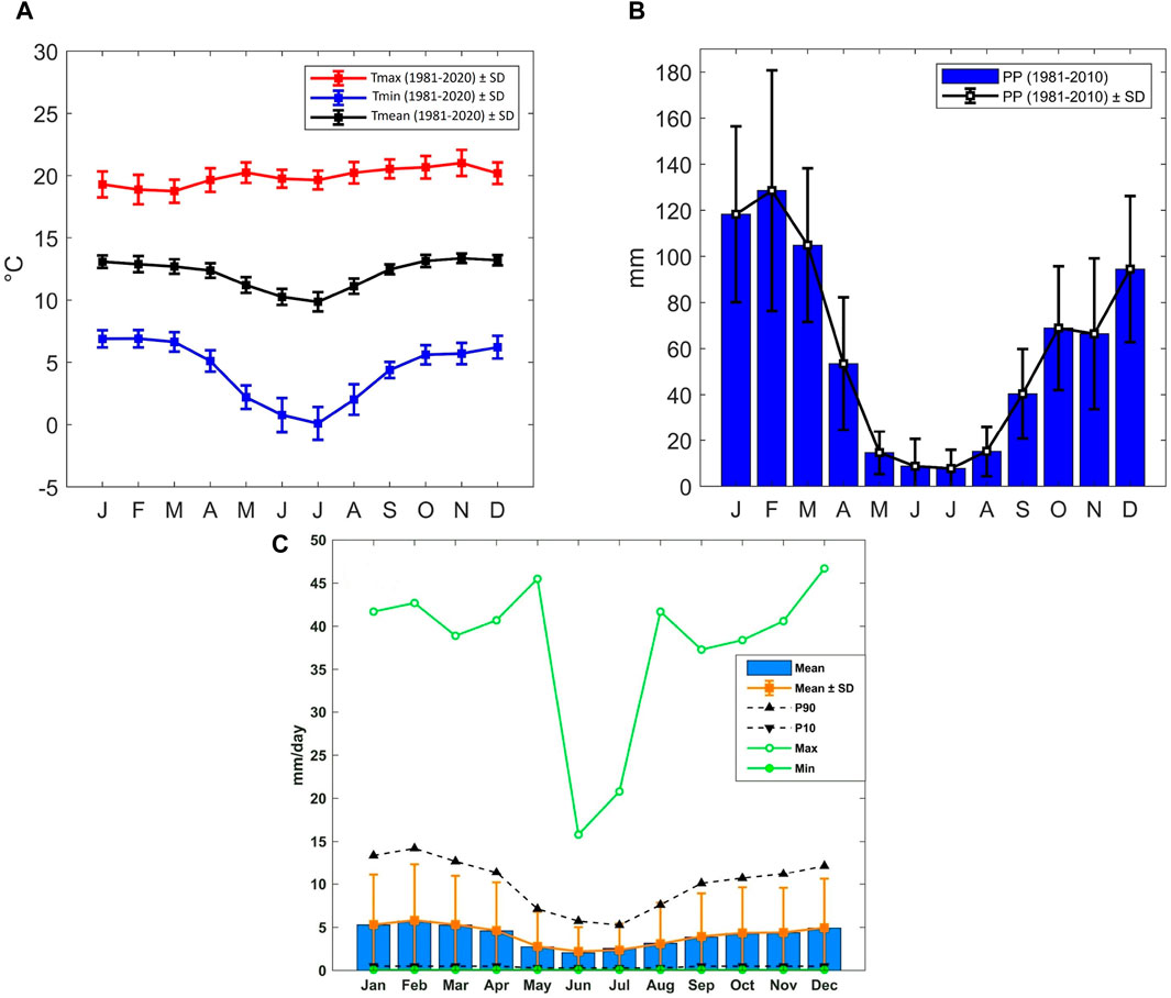
Figure 3. Seasonal variation of (A) mean, maximum and minimum of air temperature (
Another important criteria are: the precipitation of the driest month in summer is close to 90 mm
All instances of intense rainfall events on the HYGO exhibited discernible thermal meso-scale circulations linked to the South American Low-Level Jet (SALLJ). These circulations facilitated the transportation of moisture fluxes originating from both the Amazon basin in the east—traversing the passes with gentle slopes along the Andes—and the Pacific Ocean in the west. This atmospheric phenomenon unfolded in the hours leading up to the occurrence of intense rainfall events within the MV. Furthermore, our investigations revealed two primary regions on the eastern side of the Andes where moisture influxes penetrated the central Andes: one situated in the north-western region (Blue Cordillera) and the other in the south-eastern region of the Mantaro Basin.
On the western side of the Andes, several small passes with gradual slopes served as conduits for moisture fluxes originating from the Pacific Ocean (Flores-Rojas et al., 2019b). The impact of these meso-scale circulations became particularly pronounced during intense rainfall events occurring between 14 LT and 23 LT. The trajectory of these moisture flows into specific regions within the MV hinged on their interaction with circulations at medium and high atmospheric levels. Within this framework, we identified two distinct sets of atmospheric circulations that gave rise to severe rainfall events above the HYGO: the EC (East Circulation) and WC (West Circulation) events. These were characterized by the prevailing atmospheric circulations at high and medium levels, respectively (Flores-Rojas et al., 2020).
To validate the micro-climate data recorded at the HYGO automatic station (2017–2022), we compare seasonal variations in air temperature and daily accumulated precipitation with a 40-year climate normal (1981–2020) from the conventional weather station of the HYGO. This analysis ensures the representativeness and reliability of the observed micro-climate trends. In general, comparatively to the climate normal, the observations in the HYGO automatic station indicate that the climate on the HYGO during the period of 2017–2022 are very similar to the climatology values of temperature (Figure 3A), with mean maximums close to 22
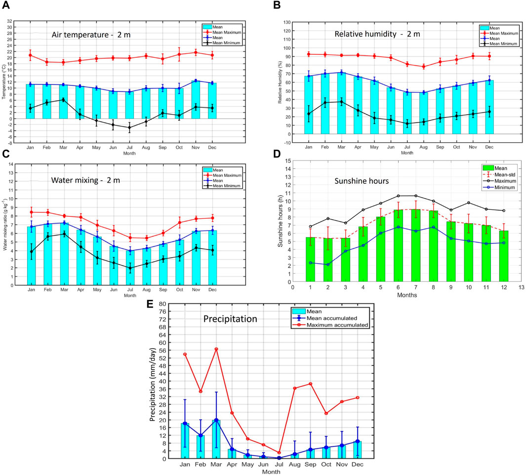
Figure 4. Seasonal variation of (A) air temperature (
Furthermore, Figure 4E illustrates the seasonal dynamics of daily accumulated precipitation from 2017 to 2022, exhibiting a pattern consistent with the 40-year precipitation climate normal depicted in Figure 3C. During this period, the maximum daily accumulated precipitation peaks in March, reaching approximately 56 mm
Finally, Figure 4C shows the seasonal variation of sunshine hours from 2017 to 2022 registered by the Heliograph installed on the HYGO (Figure 2C). Maximum values of sunshine hours are observed in June and July with values close to 10.5. It is important to note that October also has high maximum sunshine hours around to 10. This set of data is important because initial modeling work carried out around the world was involved in relating daily horizontal global irradiation to duration of bright sunshine hours.
An alternative approach to assess the representativeness of measurements obtained from the HYGO automatic station involves utilizing the psychrometric diagram for characterizing the seasonal climate conditions in the area (Gaffen and Ross, 1999). Figures 5A, B illustrate the psychrometric diagram for daily and monthly average values of specific humidity (q) (g
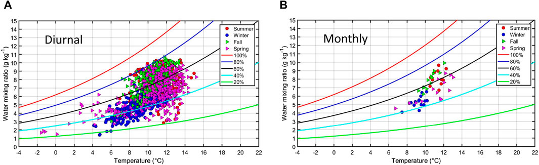
Figure 5. The psychrometric diagram for (A) daily and (B) monthly average values of specific humidity (g
Throughout all seasons, the range of daily average RH values fluctuates between 20% and 90%. The increased dispersion in the monthly average values recorded at the HYGO automatic station, particularly notable during the summer and spring, appears to be linked to climatic variability. This variability is indicative of warmer and drier conditions experienced during these seasons in recent years. Additionally, the seasonal average monthly values (Figure 5B) of q vary between 4 g
Hence, based on the climate analysis conducted herein, it can be inferred that the radiation measurements recorded between 2017 and 2022 on the HYGO automatic station might be influenced by the fact that the HYGO region experienced cooler and drier conditions during this period compared to the climatological norm. Despite these variations, as detailed in Section 5.2, it will be demonstrated that the mean behavior of
5.2 Irradiance variables
In this section, we delineate the time-integrated values of surface solar radiation components denoted by
5.2.1 Seasonal variation of hourly values
The seasonal fluctuation in the diurnal evolution of
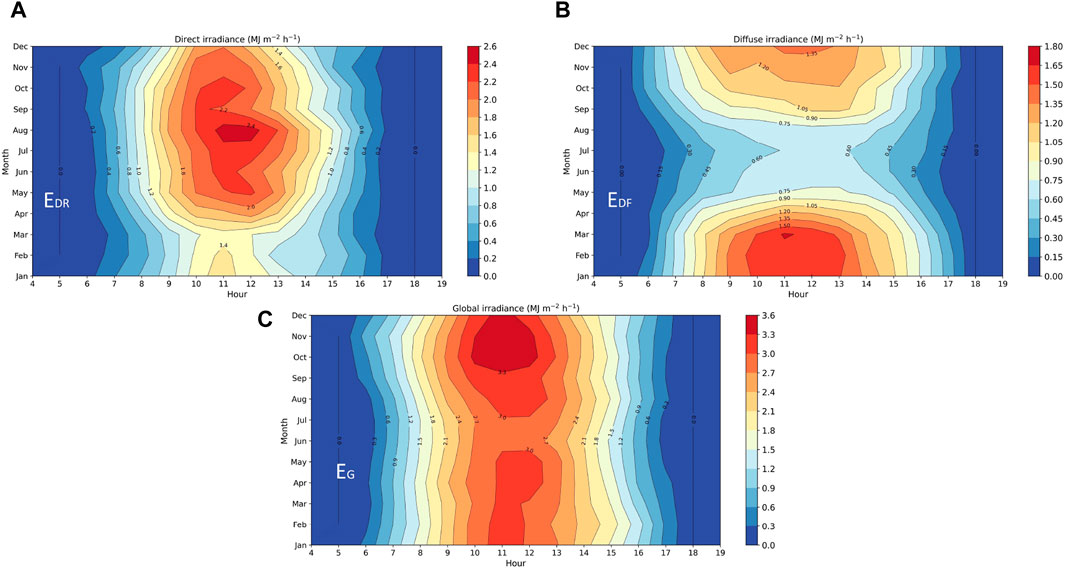
Figure 6. Seasonal and hourly cycles of average (A) direct
On the contrary, the monthly average of
The diurnal evolution of monthly average of

Figure 7. Seasonal and diurnal variation of
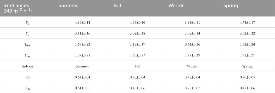
Table 1. Seasonally average hourly values of solar irradiance components:
During summer at noon,
On the other hand, during fall at noon,
It is important to highlight that for all seasons the sum of
The examination of
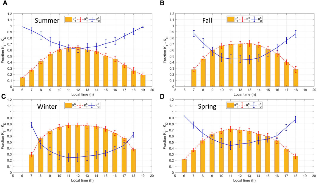
Figure 8. Diurnal variation of
5.2.2 Seasonal variation of daily values
The seasonal variation of monthly average daily values of the solar radiation components at the surface of the HYGO is presented in Figure 9A; Table 2. The highest values of
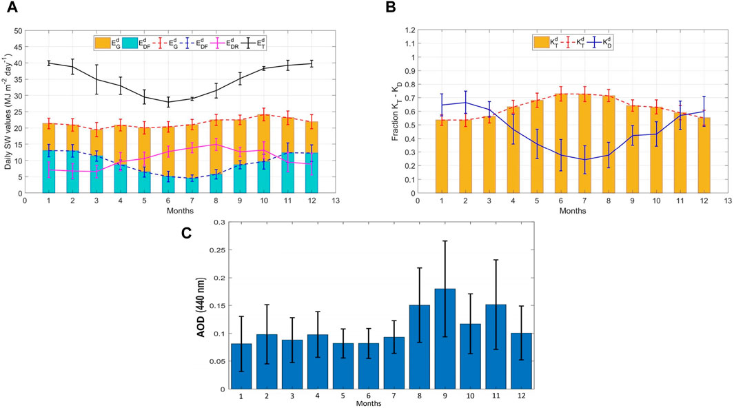
Figure 9. Monthly variation of (A) the solar irradiance components:
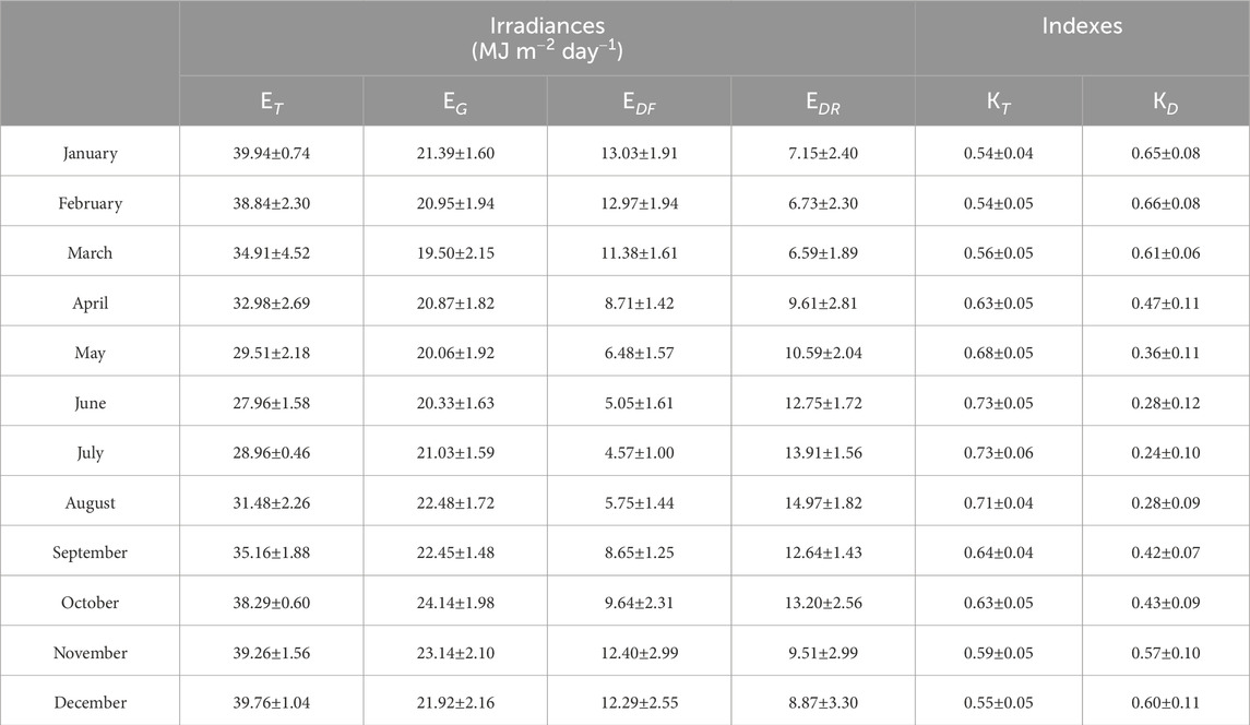
Table 2. Seasonally average daily values of solar irradiance components:
Furthermore, the seasonal evolution of
To elucidate the seasonal variations in the average daily values of solar irradiance components (
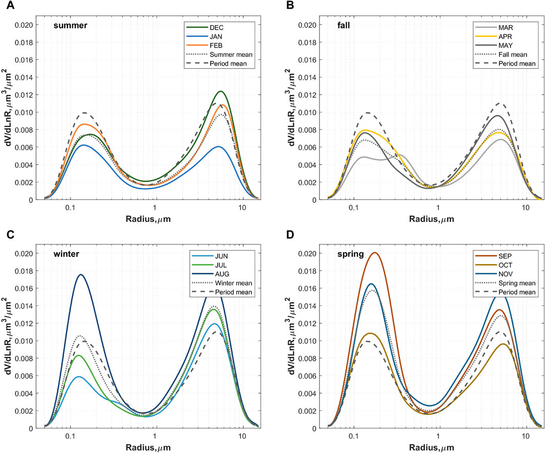
Figure 10. Monthly mean values of the aerosols volume-size distribution
During the spring season, there is a clear predominance of fine-mode aerosols, as illustrated in Figure 10D. This trend is evident in the seasonal mean (dotted line) and the monthly mean values, particularly in September and November. In September, the fine mode dominates, primarily due to aerosols generated by biomass burning in the Peruvian Amazon, which is associated with high Aerosol Optical Depth (AOD) values measured by the sun photometer at HYGO. Previous studies indicate that starting in July, AOD values rise due to biomass burning aerosols, peaking in September (Estevan et al., 2019). This increase aligns with the predominance of f ine-mode aerosols in August (Figure 10C) and throughout the spring months (Figure 10D).
In an atmosphere with aerosols, more scattered energy reaches the ground due to increased forward scattering (Iqbal, 1983). During spring, the pronounced presence of both fine-mode (0.1482 m) and coarse-mode (5.0613 m) aerosols, combined with longer daily sunshine hours and increased
Moreover, during the study period, several high aerosol concentration events were recorded by the AERONET station’s sun photometer, primarily in September. Notably, on 24 November 2020, at 21:23 UTC, the sun photometer recorded the highest AOD values since its installation on 19 March 2015, at HYGO, with an AOD 440 nm value of 1.23. These elevated AOD levels are linked to biomass-type aerosols. To determine if these aerosols were related to biomass burning, the HYSPLIT trajectory model was employed. Using NCEP reanalysis meteorological data, 120-h back-trajectories were calculated at three altitude levels: 500, 1,500, and 3000 m, from the sun photometer’s location. Figure 11 presents these back-trajectories along with fire hotspots detected by the MODIS and VIIRS satellites, indicated as red dots. By applying a coincidence criterion of a 4 km radius and 1 km height around the trajectory, two coincident fire hotspots were identified. These hotspots were located 281.2 km and 282.6 km from the sun photometer, at altitudes of 355.4 m and 343.1 m, respectively, where the 500 m back-trajectory passed. This evidence strongly suggests that the biomass-type aerosols observed on the specified date likely originated from these fire hotspots.
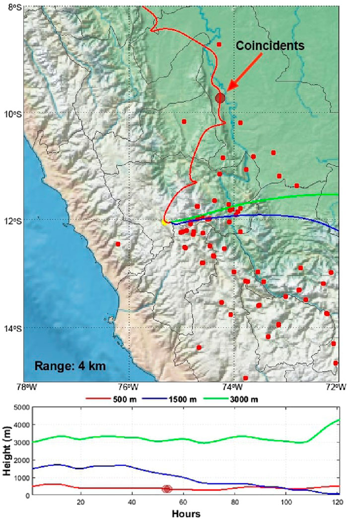
Figure 11. At the top, the red dots represent the fire hotspots associated with biomass burning. The yellow dot represents the position of the sun photometer at the HYGO, and the lines represent the back trajectories at 500 m (red line), 1,500 m (blue line), and 3000 m (green line) above the sun photometer at zero time. At the bottom, the back trajectories at different altitudes over the 120-h model run are shown.
5.3 Irradiance empirical models
Initial modeling efforts in numerous countries focused on establishing a relationship between daily horizontal global irradiation and the duration of bright sunshine. The initial phase of this endeavor entailed the formulation of regression equations based on monthly-averaged data. However, subsequent advancements have led to the development of equations utilizing data recorded at daily intervals. This progression allows for a more comprehensive understanding by connecting the discussed relationships with the daily variation between horizontal diffuse and global irradiation. This sections will present an analysis enabling the estimation of diurnal horizontal global and diffuse irradiation at different time scales.
5.3.1 Monthly-averaged daily horizontal global (MADHG) and diffuse (MADHD) irradiation models
In this section, we introduce the MADHG irradiation model, designed to establish a connection between the monthly-averaged daily clearness index (
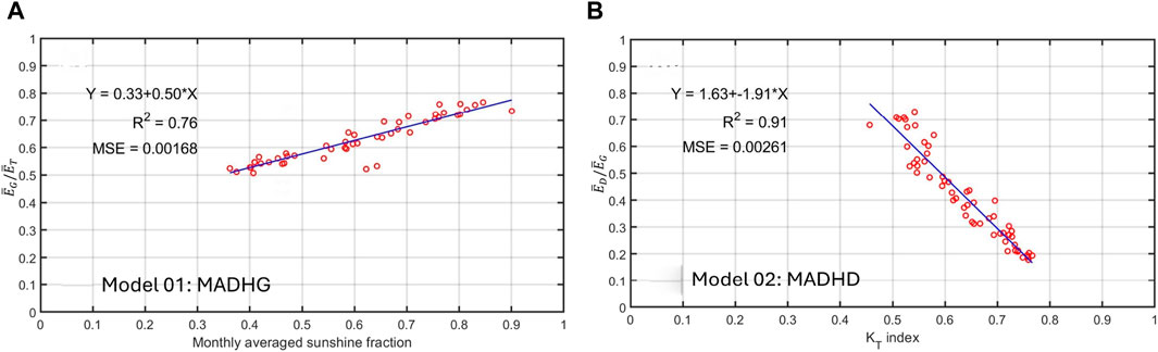
Figure 12. (A) Relationship between monthly-averaged clearness index (
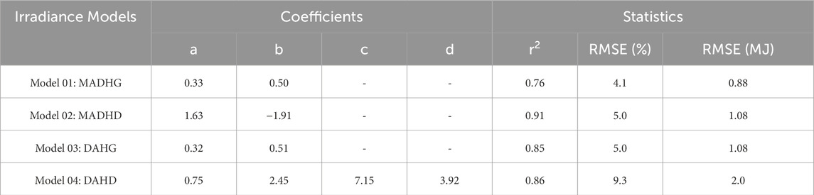
Table 3. Coefficients and statistical parameters for the empirical irradiance models. The forty percent (40%) of the total filtered dataset chosen randomly (740 days or 17 760 h) were reserved for rigorous statistical tests to evaluate model performance and robustness. The RMSE was calculated in percentage and in MJ
Furthermore, we introduced the MADHD irradiation model, designed to establish a relationship between the monthly-averaged daily diffuse ratio (
5.3.2 Daily-averaged horizontal global (DAHG) and diffuse (DAHD) irradiation models
In this section we present the irradiation model DAHG, which connect the daily clearness index (
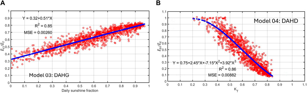
Figure 13. (A) Relationship between daily averaged clearness index (
In addition, we introduced the DAHD irradiation model, designed to establish a connection between the daily diffuse ratio (
5.3.3 Hourly horizontal global (HHG) and diffuse (HHD) irradiation models
In this section, we introduce the HHG irradiation model, which connect the ratio between the hourly global irradiation and the daily global irradiation
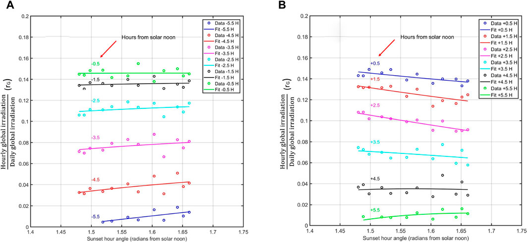
Figure 14. Ratio of hourly to daily global irradiation
Unlike certain previous studies (Liu and Jordan, 1960; Iqbal, 1983), which utilized a least-squares fit to determine the coefficients of Equations 7, 8, we employed a least-squares fit approach to ascertain these coefficients individually for each hour preceding and following solar noon. First column of Table 4 shows fitted values for the coefficients of
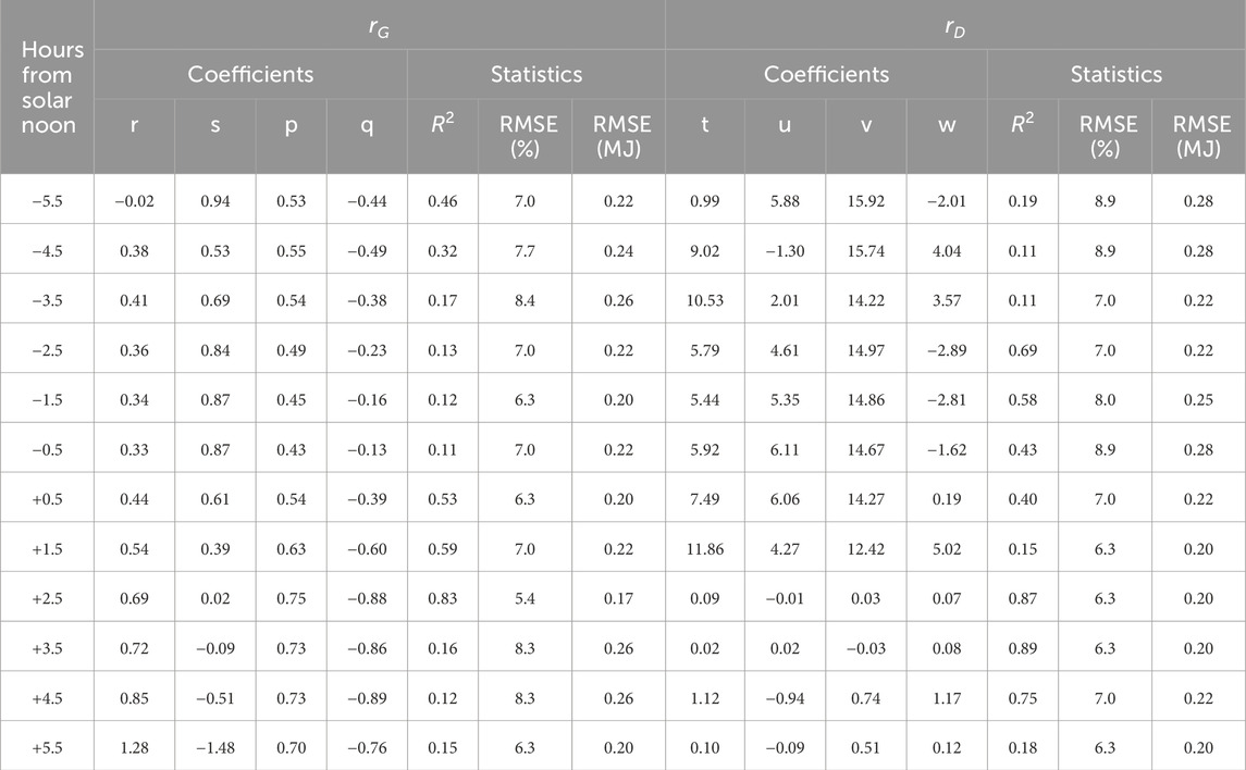
Table 4. Coefficients of
On the other hand, we also introduce the HHD irradiation model, which connect the ratio between the hourly diffuse irradiation and the daily diffuse irradiation
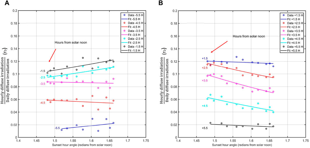
Figure 15. Ratio of hourly to daily diffuse irradiation (
Second column of Table 4 shows fitted values for the coefficients of
5.3.4 Hourly diffuse correlation (HDC) irradiance models
In this study, the sigmoid logistic function is employed to depict the correlation between
For the performance evaluation of regression models, two key statistical parameters are employed: i) the coefficient of determination
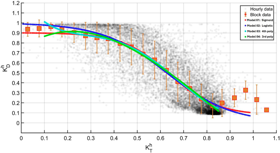
Figure 16.
The superiority of the sigmoid type 01 function becomes apparent when comparing its conformity to the block-averaged experimental curve against other correlation models (Oliveira et al., 2002a; Jacovides et al., 2006; Boland and Ridley, 2008). Notably, while the logistic function adjusted to the HYGO dataset enhanced the statistical performance of that particular model, the sigmoid function consistently outperforms all alternatives, including
The statistical parameters outlined in Table 5 indicate that all models present a coefficient of determination higher than 83%. Notably, the proposed sigmoid function fitting exhibits the best statistical performance, closely followed by the adjusted logistic and

Table 5. Equations fitted for
On the other hand, the AIC statistical method, assessed using Equations 11, 12, identifies the sigmoid function for HYGO as the best model (see Table 6). However, all correlation models are statistically relevant (
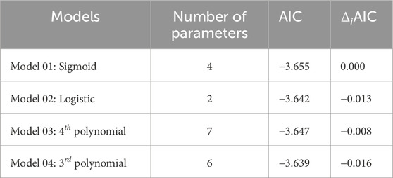
Table 6. Statistical performance of the sigmoid function model in comparison with the other empirical irradiance models for the HYGO.
6 Discussions
6.1 Atmospheric variables
The first goal of the present study was to evaluate the climate characteristics of the western Mantaro Valley, using data from two meteorological stations: the HYGO conventional station and the IGP automatic station. It includes surface weather measurements from HYGO spanning 1981 to 2020 and 1-min averages from the IGP platform between 2017 and 2022. Details on the station instrumentation are provided in recent publications (Flores-Rojas et al., 2019a; 2021; 2020).
Based on Köppen-Geiger classification (Peel et al., 2007) and data from the HYGO station, the Mantaro Valley is classified as Cwb, indicating a temperate climate with dry winters and warm summers. The criteria include a mean temperature of the hottest month above 10
An alternative method for evaluating data from the HYGO automatic station involves using psychrometric diagrams to characterize seasonal climate conditions. There are moderate correlations between specific humidity (q) and temperature (T), with approximately 60% for mean diurnal averages and 75% for mean monthly averages. Daily q values range from 1.5 g
6.2 Irradiance variables
The seasonal variation in
During the spring, moderate values of
In addition, the monthly average daily solar radiation components at the HYGO corroborate the seasonal patterns observed in hourly irradiance variables. Peak values of
Besides, the increase in AOD during September significantly raises
Moreover, the monthly mean aerosol size distributions, measured by a CIMEL CE-318T sun photometer (AERONET network) (Holben et al., 1998; 2001) reveal a bimodal distribution, with coarse-mode aerosols (5.0613
6.3 Irradiance models
The MADHG irradiation model establishes a connection between the monthly-averaged daily clearness index
Furthermore, the MADHD irradiation model is designed to establish a relationship between the monthly-averaged daily diffuse ratio (
On the other hand, the HHG irradiation model links the ratio of hourly global irradiation to daily global irradiation
Similarly, the HHD irradiation model links the ratio of hourly diffuse irradiation to daily diffuse irradiation
The correlation models for hourly diffuse irradiance utilizes several function to correlate
It is important to highlight that the clearness index
For the present study, we propose models that use the hourly clearness index
7 Conclusion
The present study evaluates the climatic characteristics of the western Mantaro Valley using data from the HYGO conventional station (1981–2020) and the IGP automatic station (2017–2022). The Mantaro Valley is classified as Cwb according to the Köppen-Geiger system, indicating a temperate climate with dry winters and warm summers. Summer sees peak precipitation, reaching 340 mm mont
The analysis of diurnal and seasonal variations in
Notably, peak values of
This study investigates irradiation models that establish robust correlations among various solar radiation parameters. The MADHG and DAHG models relate the monthly-averaged daily clearness index
It is important to emphasize that this is the first study aimed at the observational characterization and empirical modeling of global and diffuse solar irradiances in the central Peruvian Andes, using high-quality radiation data from sensors belonging to the BSRN network. In the future, this new model will be tested with
Data availability statement
The raw data supporting the conclusions of this article will be made available by the authors, without undue reservation.
Author contributions
OF-R: Writing–original draft, Methodology, Investigation, Formal Analysis, Conceptualization. JF-R: Writing–review and editing, Writing–original draft, Validation, Supervision, Methodology, Investigation, Formal Analysis, Data curation, Conceptualization. RE-A: Writing–review and editing, Validation, Supervision, Software, Formal Analysis, Data curation, Conceptualization. LG-S: Writing–review and editing, Investigation, Formal Analysis, Data curation. LS-S: Writing–review and editing, Validation, Supervision, Software, Resources, Formal Analysis. ES-P: Writing–review and editing, Software, Resources, Project administration. HK: Writing–review and editing, Visualization, Validation, Supervision, Software. YS: Writing–review and editing, Supervision, Resources, Project administration, Funding acquisition.
Funding
The author(s) declare that financial support was received for the research, authorship, and/or publication of this article. This work was done using computational resources, HPC-Linux-Cluster, from “Laboratorio de Dinámica de Fluidos Geofísicos Computacionales at Instituto Geofísico del Perú” (grants 101-2014-FONDECYT, SPIRALES2012 IRD-IGP, Manglares IGP-IDRC, PP068 program). The first author was supported by the Universidad Nacional Mayor de San Marcos – RR N° 006081-2023-R/UNMSM and project number B23131461. We also wish to thank to the “PROCIENCIA” (N° PE501080424-2022-PROCIENCIA) for the financial support during the research period, in the context to the project: Biomass Burning and Impacts in the Southern Tropics with financial scheme E070-2022-01.
Acknowledgments
This work was done using computational resources, HPC-Linux-Cluster, from “Laboratorio de Dinámica de Fluidos Geofísicos Computacionales at Instituto Geofísico del Perú” (grants 101-2014-FONDECYT, SPIRALES2012 IRD-IGP, Manglares IGP-IDRC, PP068 program). Also, we wish to thanks to the Instituto Geofísico del Perú and to the Universidad Nacional Mayor de San Marcos for logistic support for the authors during the development of the present reseach. Finally, we want to thanks to the ChatGPT 4.0 from OpenAI to improve the English style of the manuscript.
Conflict of interest
The authors declare that the research was conducted in the absence of any commercial or financial relationships that could be construed as a potential conflict of interest.
Publisher’s note
All claims expressed in this article are solely those of the authors and do not necessarily represent those of their affiliated organizations, or those of the publisher, the editors and the reviewers. Any product that may be evaluated in this article, or claim that may be made by its manufacturer, is not guaranteed or endorsed by the publisher.
References
Albarracin, G. (2017). Urban form and ecological footprint: urban form and ecological footprint: a morphological analysis for harnessing solar energy in the suburbs of cuenca, Ecuador. Energy Procedia 115, 332–343. doi:10.1016/j.egypro.2017.05.030
Álvarez, J., Mitsova, H., and Allen, H. (2011). Estimating monthly solar radiation in south-central Chile. Chil. J. Agric. Res. 71, 601–609. doi:10.4067/s0718-58392011000400016
Angstrom, A. (1924). On the computation of global radiation from records of sunshine. Ark. Geof. 2 (22), 471.
Arya, S. (2005). Micrometeorology and atmospheric boundary layer. Pure Apllied Geophys. 162, 1721–1745. doi:10.1007/3-7643-7377-6_2
Bacher, P., Madsen, H., Perers, B., and Nielsen, H. (2013). A non-parametric method for correction of global radiation observations. Sol. Energy 88, 13–22. doi:10.1016/j.solener.2012.10.024
Barragán-Escandón, E., Zalamea-León, E., Calle-Sigüencia, T.-J. J., and Terrados-Cepeda, J. (2022). Impact of solar thermal energy on the energy matrix under equatorial andean context. Energies 15 (16), 5803. doi:10.3390/en15165803
Blumthaler, M., Ambach, W., and Ellinger, R. (1997). Increase in solar uv radiation with altitude. J. Photochem. Photobiol. B Biol. 39, 130–134. doi:10.1016/s1011-1344(96)00018-8
Boland, B., and Ridley, J. (2008). Modelling solar radiation at the Earth’s surface. Springer-Verlag, 193–219.
Boor, C. (2001). in Practical g uide to splines. Applied mathematical science. Editors J. E. Marsden, and L. Sirovich (New York: Springer-Verlag), 27, 354.
Burnham, K., and Anderson, D. (2004). Multimodel inference: understanding aic and bic in model selection. Sociol. Methods and Res. 33, 261–304. doi:10.1177/0049124104268644
Ceballos, J., Porfirio, A., Oricchio, P., and Posse, G. (2022). Characterization of the annual regime of surface solar irradiance over argentine pampean region using gl1. 2 satellite-based data. Renew. Energy 194, 526–537. doi:10.1016/j.renene.2022.05.038
Cede, A., Luccini, E., Nuñez, L., Piacentini, R., and Blumthaler, M. (2002). Monitoring of erythemal irradiance in the argentine ultraviolet network. J. Geophys. Res. Atmos. 107 (AAC 1–1–AAC 1–10). doi:10.1029/2001jd001206
Codato, G., Oliveira, A., Soares, J., Escobedo, J., Gomes, E., and Pai, A. (2008). Global and diffuse solar irradiances in urban and rural areas in southeast Brazil. Theor. Appl. Climatol. 93 (1–2), 57–73. doi:10.1007/s00704-007-0326-0
Collares-Pereira, M., and Rabl, A. (1979). The average distribution of solar radiation–correlations between diffuse and hemispherical and between daily and hourly insolationvalues. Sol. Energy 22, 155–164. doi:10.1016/0038-092x(79)90100-2
Cordero, R., Seckmeyer, G., Damiani, A., Riechelmann, S., Rayas, F., Labbe, J., et al. (2014). The world’s highest levels of surface uv. Photochem. Photobiol. Sci. 13(1), 70–81. doi:10.1039/c3pp50221j
Cowley, J. (1978). The distribution over great britain of global solar radiation on a horizontal surface. Metall. Mag. 107, 357.
Della-Ceca, L., Micheletti, M. I., Freire, M., Garcia, B., Mancilla, S. G. M. A., Crinó, E., et al. (2019). Solar and climatic high performance factors for the placement of solar power plants in Argentina andes sites—comparison with african and asian sites. ASME. J. Sol. Energy Eng. 141 (4), 041004. doi:10.1115/1.4042203
De Souza, J., Lyra, C. G. B., Santos, D., Junior, C., Tiba, R. A. F., Lyra, G., et al. (2016). Empirical models of daily and monthly global solar irradiation using sunshine duration for alagoas state, northeastern Brazil. Sustain. Energy Technol. Assess. 14, 35–45. doi:10.1016/j.seta.2016.01.002
Driemel, A., Augustine, J., Behrens, K., Colle, S., Cox, C., Cuevas-Agulló, E., et al. (2018). Baseline surface radiation network (bsrn): structure and data description (1992–2017). Earth Syst. Sci. 10, 1491–1501. doi:10.5194/essd-10-1491-2018
Ellabban, O., Abu?Rub, H., and Blaabjerg, F. (2014). Renewable energy resources: current status, future prospects and their enabling technology. Renew. Sustain. Energy Rev. 39, 748–764. doi:10.1016/j.rser.2014.07.113
Erbs, D., Klein, S., and Duffie, J. (1982). Estimation of the diffuse radiation fraction for hourly, daily and monthly average global radiation. Sol. Energy 28, 293–302. doi:10.1016/0038-092x(82)90302-4
Espinoza-Villar, J., Ronchail, J., Guyot, J., Cochonneau, G., Naziano, F., Lavado, W., et al. (2009). Spatio-temporal rainfall variability in the amazon basin countries (Brazil, Peru, Bolivia, Colombia, and Ecuador). Int. J. Climatol. 29, 1574–1594. doi:10.1002/joc.1791
Estevan, R., Martínez-Castro, D., Suarez-Salas, L., Moya, A., and Silva, Y. (2019). First two and a half years of aerosol measurements with an aeronet sunphotometer at the huancayo observatory, Peru. Atmos. Environ. 3, 100037. doi:10.1016/j.aeaoa.2019.100037
Ferreira, M., Oliveira, A., Soares, J., Codato, G., Bárbaro, J., and Escobedo, E. (2012). Radiation balance at the surface in the city of são paulo, Brazil. diurnal and seasonal variations. Theor. Appl. Climatol. 107, 229–246. doi:10.1007/s00704-011-0480-2
Flores-Rojas, J., Cuxart, J., Piñas-Laura, M., Callañaupa, L. S., Suárez-Salas, , Kumar, S., et al. (2019a). Seasonal and diurnal cycles of surface boundary layer and energy balance in the central andes of perú, mantaro valley. Atmosphere 10, 779. doi:10.3390/atmos10120779
Flores-Rojas, J., Moya-Alvarez, A., Kumar, S., Martínez-Castro, D., Villalobos-Puma, E., and Silva-Vidal, Y. (2019b). Analysis of possible triggering mechanisms of severe thunderstorms in the tropical central andes of Peru, mantaro valley. Atmosphere 10 (6), 301–331. doi:10.3390/atmos10060301
Flores-Rojas, J., Moya-Alvarez, J., Valdivia-Prado, A. S., Piñas-Laura, M., Kumar, S., Karam, H., et al. (2020). On the dynamic mechanisms of intense rainfall events in the central andes of Peru, mantaro valley. Atmos. Res. 248, 105188. doi:10.1016/j.atmosres.2020.105188
Flores-Rojas, J., Silva, Y., Suárez-Salas, L., Estevan, R., Valdivia-Prado, J., Saavedra, M., et al. (2021). Analysis of extreme meteorological events in the central andes of Peru using a set of specialized instruments. Atmosphere 12, 408. doi:10.3390/atmos12030408
Frohlich, C., and Lean, J. (1998). The sun’s total irradiance: cycles, trends and related climate change uncertainties since 1976. Geophys. Res. Lett. 25, 4377–4380. doi:10.1029/1998gl900157
Gaffen, D., and Ross, R. (1999). Climatology and trends of u.s. surface humidity and temperature. J. Clim. 12, 811–828. doi:10.1175/1520-0442(1999)012<0811:catous>2.0.co;2
Garg, H., and Garg, S. (1985). Correlation of monthly-average daily global, diffuseand beam radiation with bright sunshine hours. En. Conv. Mgmt. 25, 409–417. doi:10.1016/0196-8904(85)90004-4
Giráldez, L., Silva, Y., Zubieta, R., and Sulca, J. (2020). Change of the rainfall seasonality over central Peruvian andes: onset, end, duration and its relationship with large-scale atmospheric circulation. Climate 8 (23), 23. doi:10.3390/cli8020023
Gomes, L., Marques Filho, E., Pepe, I., Mascarenhas, B. S., De Oliveira, A., De, A., et al. (2022). Solar radiation components on a horizontal surface in a tropical coastal city of salvador. Energies 15 (3), 1058. doi:10.3390/en15031058
Gueymard, C. (2005). Importance of atmospheric turbidity and associated uncertainties in solar radiation and luminous efficacy modelling. Energy 30, 1603–1621. doi:10.1016/j.energy.2004.04.040
Hastenrath, S. (1997). Measurements of solar radiation and estimation of optical depth in the high andes of Peru. Meteorl. Atmos. Phys. 64, 51–59. doi:10.1007/bf01044129
Hawas, M., and Muneer, T. (1984). Study of diffuse and global radiation characteristics in India. En. Conv. Mgmt. 24, 143–149. doi:10.1016/0196-8904(84)90026-8
Holben, B., Eck, T., Slutsker, I., Tanre, D., Buis, J., Setzer, A., et al. (1998). Aeronet – a federated instrument network and data archive for aerosol characterization. Rem. Sens. Environ. 66, 1–16. doi:10.1016/s0034-4257(98)00031-5
Holben, B., Tanré, D., Smirnov, A., Eck, T., Slutsker, I., Abuhassan, N., et al. (2001). An emerging ground-based aerosol climatology: aerosol optical depth from aeronet. J. Geophys. Res. 106 (D11), 12067–12097. doi:10.1029/2001jd900014
Huaping, L., Ming, Z., Lunche, W., Yingying, M., Wenmin, Q., and Wei, G. (2021). The effect of aerosol on downward diffuse radiation during winter haze in wuhan, China. Atmos. Environ. 265, 118714. doi:10.1016/j.atmosenv.2021.118714
Jacovides, C., Tymviosa, F., Assimakopoulos, V., and Kaltsounides, N. (2006). Comparative study of various correlations in estimating hourly diffuse fraction of global solar radiation. Renew. Energy 31, 2492–2504. doi:10.1016/j.renene.2005.11.009
Jager Waldau, A. (2019). PV status report 2019. Luxembourg: Publications Office of the European Union, 7–94.
Janjai, S., Pankaew, P., and Laksanaboonson, J. (2009). A model for calculating hourly global solar radiation from satellite data in the tropics. Appl. Energy 86, 1450–1457. doi:10.1016/j.apenergy.2009.02.005
Journee, M., and Cedric, B. (2010). Quality control of solar radiation data within the rmib solar measurements network. Sol. Energy 85, 72–86. doi:10.1016/j.solener.2010.10.021
Le Baron, B., and Dirmhirn, I. (1983). Strengths and limitations of the liu and jordanmodel to determine diffuse from global irradiance. Sol. Energy 31, 167–172. doi:10.1016/0038-092x(83)90078-6
Liu, B., and Jordan, R. (1960). The interrelationship and characteristic distribution of direct, diffuse and total solar radiation. Sol. Energy 4, 1–19. doi:10.1016/0038-092x(60)90062-1
Luccini, E., Cede, A., Piacentini, R., Villanueva, C., and Canziani, P. (2006). Ultraviolet climatology over Argentina. J. Geophys. Res. Atmos. 111. doi:10.1029/2005jd006580
Marques Filho, E., Oliveira, A., Vita, W., Mesquita, F., Codato, G., Escobedo, J., et al. (2016). Global, diffuse and direct solar radiation at the surface in the city of rio de janeiro: Observational characterization and empirical modeling. Renew. Energy 91, 64–74. doi:10.1016/j.renene.2016.01.040
Martins, F., Pereira, E., and Abreu, S. (2007). Satellite-derived solar resource maps for Brazil under swera project. Sol. Energy 81, 517–528. doi:10.1016/j.solener.2006.07.009
Maxwell, E. (1987). A quasi-physical model for converting hourly global horizontal to direct normal insolation. Golden, CO: Solar Energy Research Institute. Report SERI/TR-215-3087, –.
McKenzie, P. R. L., Aucamp, , Bais, A., Björn, L., Ilyas, M., and Madronich, S. (2011). Ozone depletion and climate change: impacts on uv radiation. Photochem. Photobiological Sci. 10(2), 182–198. doi:10.1039/c0pp90034f
Monteith, J., and Unsworth, M. (1990). Principles of environmental Physics. London: Edward Arnold, 291 edn. first.
Motulsky, H., and Arthur, C. (2003) “Fitting models to biological data using linear and nonlinear regression: a practical guide to curve fitting. New York, NY: online edn, Oxford Academic. doi:10.1093/oso/9780195171792.001.0001 (Accessed 01 August, 2024)
Muneer, T., and Hawas, M. (1984). Correlation between daily diffuse and global radiation for India. En. Conv. Mgmt. 24, 151–154. doi:10.1016/0196-8904(84)90027-x
Oliveira, A., Machado, A., Escobedo, J., and Soares, J. (2002a). Correlation models of diffuse solar-radiation applied to the city of São Paulo, Brazil. Appl. Energy 71, 59–73. doi:10.1016/s0306-2619(01)00040-x
Oliveira, A., Machado, A., Escobedo, J., and Soares, J. (2002b). Diurnal evolution of solar radiation at the surface in the city of s/ao paulo: seasonal variation and modeling. Theor. Appl. Climatol. 71, 213–250. doi:10.1007/s007040200007
Page, J. (1977). The Estimation of monthly mean Value of daily short wave Irradiation on Vertical and inclined Surfaces from sunshine Records for latitudes 60°N to 40°S. Department of Building Science, University of Sheffield, UK.
Peel, M., Finlayson, B., and McMahon, T. (2007). Updated world map of the Köppen-Geiger climate classification. Hydrol. Earth Syst. Sci. 11, 1633–1644. doi:10.5194/hess-11-1633-2007
Pereira, E., Martins, F., Abreu, S., and Colle, S. (2006). Brazilian atlas for solar energy resource: swera results, são josé dos campos. INPE 01, 60.
Perez, R., Ineichen, P., Maxwell, E., Seals, R., and Zelenka, A. (1992). Dynamic global to direct irradiance conversion models. ASHRAE Trans. 98, 354–369.
Perez, R., Ineichen, P., Seals, R., and Zelenka, A. (1990). Making full use of the clearness index for parameterizing hourly insolation conditions. Sol. energy 45, 111–114. doi:10.1016/0038-092x(90)90036-c
Piazena, H. (1996). The effect of altitude upon the solar uv-b and uv-a irradiance in the tropical chilean andes. Sol. Energy 57, 133–140. doi:10.1016/s0038-092x(96)00049-7
Podestá, G., Núñez, L., Villanueva, C., and Skansi, M. (2004). Estimating daily solar radiation in the argentine pampas. Agric. For. meteorology 123, 41–53. doi:10.1016/j.agrformet.2003.11.002
Redweik, P., Catita, C., and Brito, M. (2013). Solar energy potential on roofs and facades in an urban landscape. Sol. Energy 97, 332–341. doi:10.1016/j.solener.2013.08.036
Reindl, D., Beckman, W., and Duffie, J. (1990). Diffuse fraction correlations. Sol. Energy 45, 1–7. doi:10.1016/0038-092x(90)90060-p
Ridley, B., Boland, J., and Lauret, P. (2010). Modelling of diffuse solar fraction with multiple predictors. Renew. Energy 35, 478–483. doi:10.1016/j.renene.2009.07.018
Rodríguez-Hidalgo, M., Rodríguez-Aumente, P., Lecuona, A., Legrand, M., and Ventas, R. (2012). Domestic hot water consumption vs. solar thermal energy storage: the optimum size of the storage tank. Appl. Energy 97, 897–906. doi:10.1016/j.apenergy.2011.12.088
Saluja, G., Muneer, T., and Smith, M. (1988). Methods for estimating solar irradiation on a horizontal surface. Ambient. Energy 9, 59–74. doi:10.1080/01430750.1988.9675915
Saluja, G., and Robertson, P. (1983). Design of passive solar heating in the northern latitude locations. Perth: Proc. Solar World Congress, 40.
Sayigh, A. (2020). Solar and wind energy will supply more than 50electricity by 2030 Berlin/Heidelberg, Germany: Springer, 385–399.
Silva, Y., Takahashi, K., and Chavez, R. (2008). Dry and wet rainy seasons in the mantaro river basin (central peruvian andes). Adv. Geosci. 14, 261–264. doi:10.5194/adgeo-14-261-2008
Silva, Y., and Trasmonte, G. (2010). Variabilidad de las lluvias en el valle del Mantaro Memoria del Subproyecto: Pronóstico estacional de lluvias y temperatura en la cuenca del río Mantaro para su aplicación en la agricultura (Fondo Editorial CONAM-Instituto Geofísico del Perú). primera edn.
Skartveit, A., and Olseth, J. (1987). A model for the diffuse fraction of hourly global radiation. Sol. Energy 38, 271–274. doi:10.1016/0038-092x(87)90049-1
Skartveit, A., Olseth, J., and Tuft, M. (1998). An hourly diffuse fraction model with correction for variability and surface albedo. Sol. Energy 63, 173–183. doi:10.1016/s0038-092x(98)00067-x
Smietana, P., Flocchini, R., Kennedy, R., and Hatfield, H. (1984). A new look at the correlation of Kd and Kt ratios and at global solar radiation tilt models using one-minute measurements. Sol. Energy 32, 99–107. doi:10.1016/0038-092x(84)90053-7
Suárez Salas, L., Flores-Rojas, J. L., Pereira Filho, A. J., and Karam, H. (2017). Ultraviolet solar radiation in the tropical central Andes (12.0°S). Photochem. Photobiol. Sci. 16, 954–971. doi:10.1039/c6pp00161k
Supit, I., and Van Kappel, R. (1998). A simple method to estimate global radiation. Sol. Energy 63, 147–160. doi:10.1016/s0038-092x(98)00068-1
Turton, S. (1987). The relationship between total irradiation and sunshine duration in the humid tropics. Sol. Energy 38, 353–354. doi:10.1016/0038-092x(87)90007-7
Vuilleumier, L., Hauser, M., Felix, C., Vignola, F., Blanc, P., Kazantzidis, A., et al. (2014). Accuracy of ground surface broadband shortwave radiation monitoring. J. Geophys. Res. Atmos. 119, 13838–13860. doi:10.1002/2014jd022335
Whillier, A. (1956). The determination of hourly values of total solar radiation from daily summations. Arch. Metall. Geoph. Biokl. 7, 197–204. doi:10.1007/bf02243322
Woodward, F., and Sheeh, J. (1983). Principles and measurements in environmental biology. London: Butterworth Co, 263.
Younes, S., Claywell, R., and Muneer, T. (2005). Quality control of solar radiation data: present status and proposed new approaches. Energy 30, 1533–1549. doi:10.1016/j.energy.2004.04.031
Zaratti, F., Forno, R. N., García Fuentes, J., and Andrade, M. (2003). Erythemally weighted uv variations at two high-altitude locations. J. Geophys. Res. Atmos. 108. doi:10.1029/2001jd000918
Glossary

Keywords: solar irradiance models, global irradiance, diffuse irradiance, direct irradiance, peruvian central Andes
Citation: Fashé-Raymundo O, Flores-Rojas JL, Estevan-Arredondo R, Giráldez-Solano L, Suárez-Salas L, Sanabria-Pérez E, Karam HA and Silva Y (2024) Observational characterization and empirical modeling of global, direct and diffuse solar irradiances at the Peruvian central Andes. Front. Earth Sci. 12:1399971. doi: 10.3389/feart.2024.1399971
Received: 12 March 2024; Accepted: 19 July 2024;
Published: 13 August 2024.
Edited by:
Huade Guan, Flinders University, AustraliaReviewed by:
Eduardo Landulfo, Instituto de Pesquisas Energéticas e Nucleares (IPEN), BrazilJianhui Bai, Chinese Academy of Sciences (CAS), China
Copyright © 2024 Fashé-Raymundo, Flores-Rojas, Estevan-Arredondo, Giráldez-Solano, Suárez-Salas, Sanabria-Pérez, Karam and Silva. This is an open-access article distributed under the terms of the Creative Commons Attribution License (CC BY). The use, distribution or reproduction in other forums is permitted, provided the original author(s) and the copyright owner(s) are credited and that the original publication in this journal is cited, in accordance with accepted academic practice. No use, distribution or reproduction is permitted which does not comply with these terms.
*Correspondence: José Luis Flores-Rojas, amZsb3Jlc0BpZ3AuZ29iLnBl