Ocean component of the first operational version of Hurricane Analysis and Forecast System: Evaluation of HYbrid Coordinate Ocean Model and hurricane feedback forecasts

The first operational version of the coupled Hurricane Analysis and Forecast System (HAFSv1) launched in 2023 consists of the HYbrid Coordinate Ocean Model (HYCOM) and finite-volume cubed-sphere (FV3) dynamic atmosphere model. This system is a product of efforts involving improvements and updates over a 4-year period (2019–2022) through extensive collaborations between the Environmental Modeling Center at the US National Centers for Environmental Prediction (NCEP) and NOAA Atlantic Oceanography and Meteorology Laboratory. To provide two sets of numerical guidance, the initial operational capability of HAFSv1 was configured to two systems—HFSA and HFSB. In this study, we present in-depth analysis of the forecast skills of the upper ocean that was co-evolved by the HFSA and HFSB. We chose hurricane Laura (2020) as an example to demonstrate the interactions between the storm and oceanic mesoscale features. Comparisons performed with the available in situ observations from gliders as well as Argos and National Data Buoy Center moorings show that the HYCOM simulations have better agreement for weak winds than high winds (greater than Category 2). The skill metrics indicate that the model sea-surface temperature (SST) and mixed layer depth (MLD) have a relatively low correlation. The SST, MLD, mixed layer temperature (MLT), and ocean heat content (OHC) are negatively biased. For high winds, SST and MLT are more negative, while MLD is closer to the observations with improvements of about 8%–19%. The OHC discrepancy is proportional to predicted wind intensity. Contrarily, the mixed layer salinity (MLS) uncertainties are smaller and positive for higher winds, probably owing to the higher MLD. The less-negative bias of MLD for high winds implies that the wind-force mixing is less effective owing to the higher MLD and high buoyancy stability (approx. 1.5–1.7 times) than the observations. The heat budget analysis suggests that the maximum heat loss by hurricane Laura was O(< 3°C per day). The main contributor here is advection, followed by entrainment, which act against or with each other depending on the storm quadrant. We also found relatively large unaccountable heat residuals for the in-storm period, and the residuals notably led the heat tendency, meaning that further improvements of the subscale simulations are warranted. In summary, HYCOM simulations showed no systematic differences forced by either HFSA or HFSB.

1 Introduction

The US National Centers for Environmental Prediction (NCEP) has a long history of developing coupled regional hurricane–ocean forecast systems and running operationally with the goal of providing improved numerical guidance to hurricane specialists at the National Hurricane Center (NHC) since 2001. Over the past two decades, a new system has replaced the old system with improved/advanced physics, coupling, high resolution, nesting, and data assimilation. For example, the Geophysical Physical Dynamics Laboratory (GFDL) Hurricane Prediction System was decommissioned in 2014, and the hurricanes in a multiscale ocean-coupled non-hydrostatic model (HMON) was used to maintain continuity for the NHC official forecasts, with higher-resolution nesting and eddy-resolving ocean model coupling. The Hurricane Weather and Forecast System (HWRF) has been operated as another regional system in the NCEP product suites, and its high forecasting skills have been widely acknowledged by operational forecasters, including the US Navy’s Joint Typhoon Warning Center (JTWC), which is attributed to the advancements made through collaborations between scientists at the Environmental Modeling Center (EMC) and research community, with support from the NOAA Hurricane Forecast Improvement Program (HFIP). Similarly, a new-generation Hurricane Analysis and Forecast System (HAFS) replaced the legacy HWRF and HMON, with operations commencing in June 2023.

The HAFS development started in 2019 and was built to the initial operational capability (IOC) for the coupled hurricane–ocean modeling system (Zhang et al., 2023). After 4 years of extensive developmental efforts, including real-time tests in each hurricane season followed by updates for further improvements, the IOC was transitioned to the first operational version of the numerical guidance model HAFSv1 in June 2023. This version has two configurations, namely HFSA and HFSB. To maintain diversity, the models have different configurations of the model physics. Large-scale retrospective tests of the North Atlantic hurricanes from the 2020 to 2022 seasons show approximately 12% higher tracking skills than the HWRF (H221 in Figure 1A). The intensity (defined by a 1-min sustained maximum wind speed denoted as Vmax) skills (Figure 1B), on the other hand, are mixed and are poor/better for early/late lead times than the HWRF (H221 in Figure 1B). The HAFSv1 also outperforms HMON (M221) for both track (Figure 1A) and intensity predictions (Figure 1B). Between HFSA and HFSB, the former has higher tracking skill by ≤ 8% (at 72 h) for the entire lead time, except for brief periods of 36 and 42 h for poor skills ≤1%. The HFSA also has better skills at intensity forecasting (by < 6%) for the first 42 h of lead time, but the HFSB shows persistently high skills after the 48 h point (<9.5%).

Figure 1

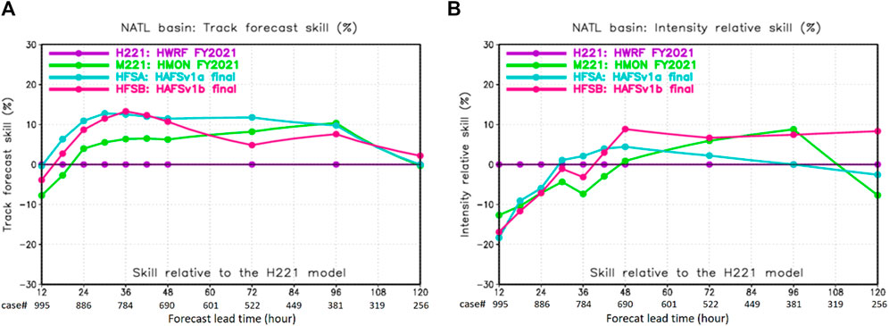
Figure 1. Skill comparisons of the two latest configurations of the HAFS (HFSA and HFSB) with operational HMON (M221) relative to the operational HWRF (H221) for (A) tracking and (B) intensity (1-min sustained maximum wind, Vmax) as functions of the forecast lead time in hours and number of cases. The statistical results were generated for a total of 995 homogeneous cases (at a 12-h forecast lead time) encompassing three hurricane seasons (2020–2022) in the North Atlantic basin. The graphics were generated using the National Hurricane Center (NHC) verification package.

One of the roles of the HYbrid Coordinate Ocean Model (HYCOM) in HAFSv1 is to support accurate simulations of air–sea interaction processes by exchanging updated state variables with the finite-volume cubed-sphere (FV3) model components. The HYCOM has been widely used and extensively tested by the research community. Because it is an operational ocean forecast model in the US Navy Fleet Numerical Meteorology and Oceanography Center (FNMOC) (Chassignet et al., 2007; Burnett et al., 2014; Metzger et al., 2014) and a backbone model supported by multiple institutions sponsored by the National Ocean Partnership Program (NOPP) as part of the US Global Ocean Data Assimilation Experiment (Chassignet et al., 2007), the leveraged efforts have contributed to significant improvements to HYCOM, including data assimilation (DA) (Cumming, 2005; Cummings and Smedstad, 2013). The HYCOM has also been popularly used to study physical processes at the regional (Heffner et al., 2008; Subrahmanyam et al., 2009;) and larger scales (Kara et al., 2005; Rasmussen et al., 2011; Wang et al., 2015). There are also numerous research studies that have examined and tested its validity for mixing physics under different environments (Halliwell, 2004; Kara et al., 2008; Kara et al., 2010; Pottapinjara and Joseph, 2022; Zamudio and Hogan, 2008).

HYCOM also serves as an operational ocean forecast system in the US NCEP, starting from an earlier operational version of the Atlantic Real-Time Forecast System (RTOFS) (Mehra and Rivin, 2010) to the global RTOFS. At present, the global system is operated daily as part of the NCEP product suite to produce weather-scale ocean products, including 2 days of nowcasts and 8 days of forecasts at 6-h intervals. The system temporally integrates the initial conditions assimilated with timely available observations by the flow-dependent 3DVar DA algorithm (Cummings, 2005; Garraffo, et al., 2020). The regional HYCOM configuration leverages the in-house global RTOFS to seamlessly obtain initial and boundary conditions for the cycling forecast system for coupled regional hurricane systems, such as the HWRF and HMON. Its skills for two-way coupling were documented by Kim et al. (2014) and three-way ocean–hurricane–wave coupling were reported by Kim et al. (2022).

In the present work, we document the application of a regional HYCOM to support two-way interactions for the HAFS as well as assessments of the forecast skills of HFSA and HFSB. We show validations and analyses with data from hurricane Laura (2020 season) selected from large-scale tests. The reason for this choice is that the Gulf of Mexico (GOM) has a variety of oceanic features that modulate the sea-surface temperature (SST) feedback and is a region where many landfalling storms have resulted in damage and casualties in the past owing to the warm upper oceanic conditions in favor of tropical cyclone (TC) intensification. Hurricane Laura underwent two phases of rapid intensification (RI) when transiting over the semi-enclosed basin. The GOM entails various mesoscale features, such as warm loop currents (LCs), warm/cold core eddies, and freshwater barriers, which could enhance the enthalpy exchanges by the perennially warm SST of the GOM. In Section 2, we briefly introduce the HAFS for the Unified Forecast System (UFS) framework and component models. Section 3 describes the data and analysis methods, along with brief descriptions of two cases of interest. Section 4 presents the results of this study, and Section 5 summarizes the findings and discussion.

2 Hurricane analysis and forecast system

Figure 2 is a schematic describing the HAFS in the UFS framework. The model includes the FV3 atmosphere and HYCOM components for the ocean. The coupling components are the Earth system modeling framework (ESMF) and National Unified Operational Prediction Capability (NUOPC) that are located at the upper level of each component model and activated by a wrapper under the Community Mediator for Earth Prediction Systems (CMEPS).

Figure 2

Figure 2. HAFS model components and data flow with the atmospheric data assimilation (ATM-DA) module. The exchange variables are shown in italics between the HYCOM and FV3 model via the Community Mediator for Earth Prediction Systems (CMEPS). Sources for the initial and boundary conditions (ICs and BCs) for FV3 and HYCOM are included. Flux includes the wind stress, net shortwave radiation, net longwave radiation, latent heat flux, and sensible heat flux. Prate and MSLP denote the precipitation rate and mean sea-level pressure, respectively.

The atmospheric model is based on the FV3 dynamic core (Lin and Rood, 1996; Lin, 2004) with a choice of a physics suite from the Common Community Physics Package (CCPP). The configuration involves one quasi-stationary parent domain at a grid spacing of ∼6 km on the Extended Schmidt Genomic grids (Purser et al., 2020) and typical horizontal dimensions of 1,320 by 1,200, with a moving nest following a storm of interest one at a time at a resolution of ∼2 km over the 600×600 dimensions. Two-way nesting was performed using the flexible modeling system (FMS) between the stationary (parent) and moving (nested) domains. Figure 3 shows an example of the atmospheric coverage (shaded boxes) to provide numerical predictions of the TCs over the World Meteorological Organization (WMO) Regional Tropical Cyclone bodies (https://community.wmo.int/en/tropical-cyclone-regional-bodies) around the globe. Only the parent domain has direct communication with the ocean. The solution in the vertical direction is obtained from 81 layers at 20 m above the mean sea level to the 10 hPa model top. To improve the subset of initial conditions (ICs) from the coarse resolution of the FV3-based Global Forecast System (GFS) analysis, the HAFS employs 4DEnVar with background error covariance from the Global Data Assimilation System (GDAS) and vortex initialization. The boundary conditions (BCs) are the interpolated GFS forecast products. The CCPP is one of the UFS modules that supports various physics schemes, including the planetary boundary layer (PBL) physics, microphysics, radiation, cumulus convection, and gravity wave drag, for the atmospheric model (Wang et al., 2024; companion paper). The surface to boundary-layer physics for the HAFSv1 is specially tailored for application to TCs, where the turbulence fluxes are updated using the SST and bulk exchange coefficients empirically defined as functions of 10-m winds (Biswas et al., 2018). The details of the physics schemes may be found in Wang et al. (2024), and detailed differences between the HFSA and HFSB configurations may be found in Zhang et al. (2023).

Figure 3

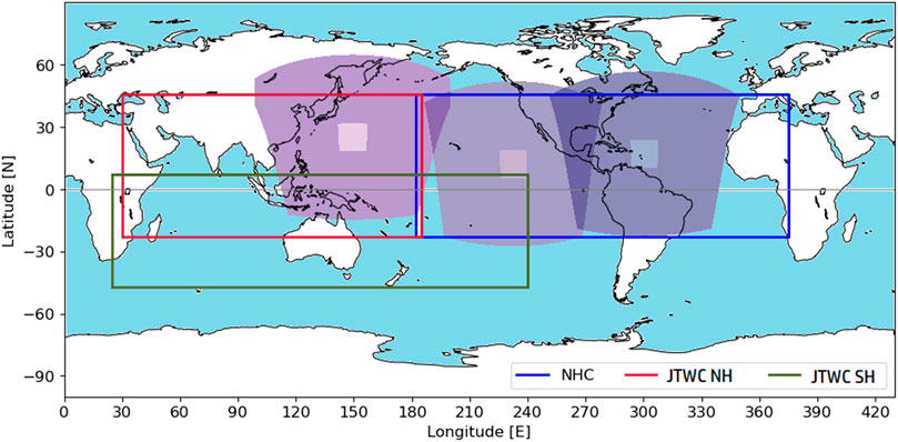
Figure 3. HYCOM basin domains for hurricanes in the North Atlantic and East/Central North Pacific basins, which are the areas of responsibility for the forecasters at the NHC and Central Pacific Hurricane Center (NHC; blue box); typhoons in the Western North Pacific and North Indian basins (JTWC NH; red box) and for Cyclones in the South Indian and Pacific basins (JTWC SH; green box) are the responsibility of the forecasters at the Joint Typhoon Warning Center (JTWC). Shaded areas are examples of the FV3 parent and nested domains of each basin.

The HYCOM is an eddy-resolving ocean general circulation model that solves 3D primitive equations in an Arakawa C-grid at a resolution of 1/12 degrees on the Mercator projection and 41 hybrid z-isopycnic vertical coordinates (Bleck, 2002; Chassignet et al., 2007; Chassignet et al., 2020). These regional domains are shown in Figure 3, covering the tropics in both the Northern and Southern hemispheres, with dimensions of 2,413 by 964 for the area of responsibility for forecasters at the NHC (blue box) as well as 1,938 by 937 (JTWC NH; red box) and 2,689 by 756 (JTWC SH; green box) for the JTWC.

The HYCOM for regional applications has the same numerical configuration as that of the global RTOFS to utilize the readily available data in the real-time computational environment for providing ICs on the fly without remapping, interpolation, or delayed computations. Solutions over the non-overlapping areas are obtained by one-way forcing as the ocean preparation step before forecast integration. These are subsets of the 3-h global FV3 products of wind stress components, net shortwave radiation, net longwave radiation, latent heat flux, sensible heat flux, precipitation rate (Prate in Figure 2), and mean sea-level pressure (MSLP in Figure 2). Vertical mixing is based on non-local k-profile parameterization (KPP; Large et al., 1994), with a background viscosity of 3 × 10⁻⁵ m² s⁻¹ and diffusivity of 10⁻⁵ m² s⁻¹. The shear instability is restricted by the maximum allowed values of 5 × 10⁻⁵ m² s⁻¹ for both the viscosity and diffusivity and a maximum gradient Richardson number of 0.7. Lateral mixing uses a Laplacian operator that is a deformation-dependent eddy viscosity with a velocity scale factor of 0.05 m s⁻¹.

The ICs are different for the 00Z and rest cycles; the ICs for the 00Z cycle, for example, are a simple subset of the global RTOFS 3D restart file composed of temperature (T), salinity (S), east (u) and north velocity components (v), and layer thicknesses from the 24-h nowcast. For the other cycles, we combine the 00Z analysis field with the 6, 12, and 18 h forecasts to retain the assimilated state variables for the time integration. The lateral BCs are closed but relaxed to the climatology, and the ICs are integrated at 120 and 10 s using the explicit–implicit splitting-model solutions with forcing exported from the FV3 component model by the CMEPS at 360 s intervals (Figure 2). The dynamically updated SST field is passed to the FV3 at the same 360 s coupling time (Figure 2) for the surface boundary layer module to update the momentum and enthalpy flux using the bulk exchange coefficients based on the empirical relationship of the roughness length scale and wind speeds [Figure 2 in Kim et al. (2022)].

3 Data and methodology

3.1 Hurricane forecast data

Model outputs were produced in 3D volume data of the diagnostic and prognostic variables in the netCDF format at 3-h intervals for the FV3 and in the binary format at 6-h intervals for the HYCOM. Additional postprocessing was employed to convert some of the atmospheric variables to grib2 files and the oceanic variables including MLD, 26°C isotherm, and ocean heat content (OHC) to netCDF files. One important postprocessing step is producing numerical guidance, which is achieved with the GFDL vortex tracker (Marchok, 2021).

On-time delivery of numerical products is critical to the operational environment. To meet the real-time requirements, extensive profiling was performed, including optimizations of the codes, tiling, and number of cores. Supplementary Appendix S1 provides more details, including the individual workflow steps, execution timings, and required numbers of cores.

The guidance model outputs produced by the vortex tracker include a set of six hourly TC center locations; Vmax; minimum sea-level pressure (Pmin); radius of the maximum wind (RMW); as well as 34-kt (R34), 50-kt (R50), and 64-kt (R64) winds in each quadrant. The verifications were performed using the NHC verification tools with the NHC’s Best Track data. The results for the total of 1,091 homogeneous cases over three hurricane seasons (2020–2022) suggest that HAFSv1 statistically performs better than the legacy models HWRF and HMON, especially for lead times from 18 h for tracking and from 30 h (HFSA)/42 h (HFSB) for intensity (Figure 1). The Vmax intensity bias ranges between −2.5 and 1.5 kt (Figure 4A) and is comparable with that of the HWRF but better than that of the HMON that has a negative trend with lead time. Conversely, the Pmin bias is consistently negative throughout the lead time, with magnitudes of less than −4 hPa. The Pmin bias of HAFSv1 is similar to that of the HWRF (Figure 4B), whereas none of the models outperform the HMON. Overall, it is suggested that the wind-pressure relationships for models except the HMON are approximately similar to those of the observed data.

Figure 4

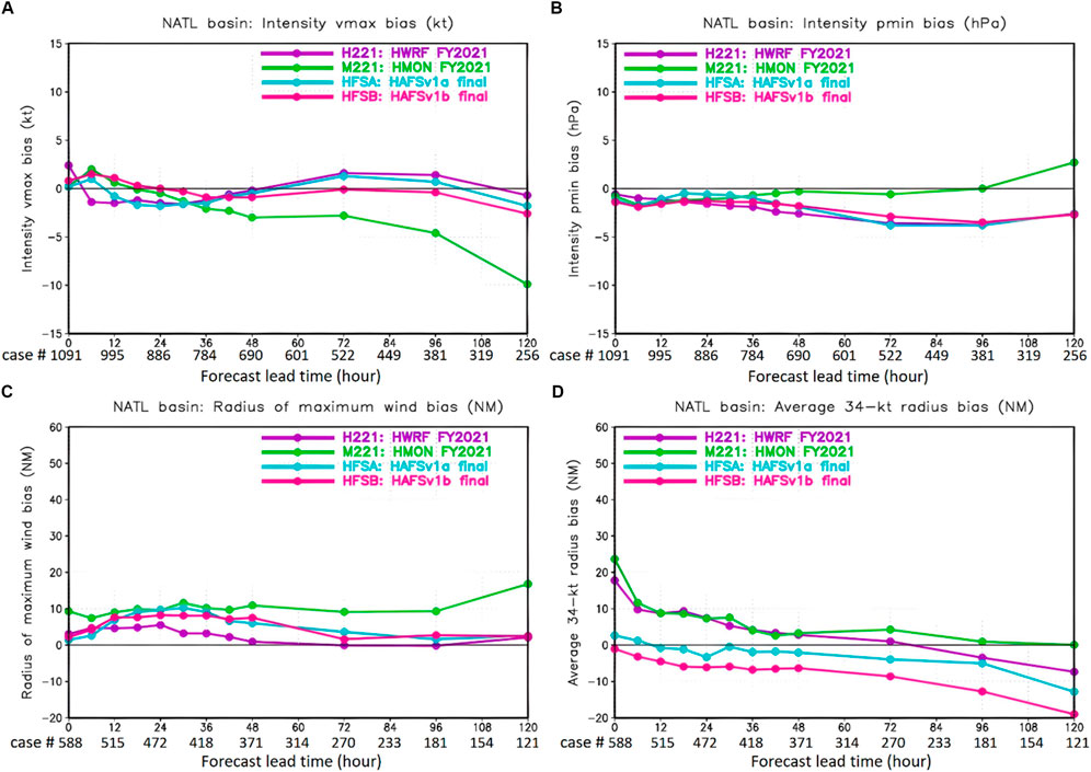
Figure 4. Bias comparisons of (A) Vmax, (B) Pmin, (C) radius of the maximum wind (RMW), and (D) radius of the 34-kt wind (R34) for HFSA and HFSB against the HWRF (H221) and HMON (M221). The units are kt, hPa, and nautical mile (NM) for (A), (B), and (C, D), respectively. A total of 1,091 homogeneous cases were verified against the best track (BT).

In general, HAFSv1 predicts a larger bias of the RMW compared to those for the HWRF and HMON, with a maximum of ∼10/8 NM for the HFSA/HFSB, while the HWRF and HMON match the observations for the best and worst cases, respectively (Figure 4C). On the contrary, the outermost TC sizes (R34) for the HFSA and HFSB start with almost zero biases but gradually grow smaller in the lead time and reach maximum negative biases at 120 h (Figure 4D). Between the HFSA and HFSB, the HFSA R34 agrees with the observed size at an average of < 5 NM than the HFSB. As for the R50 and R64 (not shown), both HFSA and HFSB show similar predictions with better agreement with the observations compared to the HWRF and HMON.

To avoid redundancy in this work, we chose an exemplary storm from our samples that undergoes various TC stages and contacts diverse oceanic conditions. Hurricane Laura from the year 2020 fits these specifications: the storm achieved at least four landfalls during its heading toward the GOM from the major development region (MDR) but maintained Tropical Storm (TS) strength over the period. The intensity at the time it entered the GOM was 60 kt, but the storm gradually intensified to 75 kt as it transited the LC of the warm body of water, followed by RI to a Category 4 hurricane (130 kt) at 00Z on 27 August 2020. During its final landfall at Cameron, Louisiana (approximately 06Z on August 27), the intensity remained that of a Category 4 hurricane.

The GOM is a semi-enclosed ocean and a unique place where a TC can make a complete transit in as short a duration as 2.5 days at a typical moving speed while experiencing various oceanic features, such as warm LCs, cold/warm core eddies, and freshwater barriers often offshore advected from the Mississippi river discharge (Da Silva and Castelao, 2018). These features often play crucial roles in TC intensification via air–sea interactions, particularly modulating the enthalpy flux and probably influencing the intensity changes of the TC. Conversely, the ocean is also influenced by the storms and probably retains their impacts for a while to eventually impact the general circulation in the GOM and the following storm (Avila-Alonso et al., 2020; Eley et al., 2021; Gong et al., 2023).

3.1.1 Hurricane Laura (2020)

A tropical depression was first classified around 00Z on 20 August 2020 about 850 NM east–southeast of Antigua (Pasch et al., 2021). Soon after, it underwent repetitive cycles of organization/disorganization until it became a tropical storm at around 00Z August 22. While moving parallel to the southern part of the Greater Antilles Island chain, it gained strength to ∼45 kt (Figure 5). At the time when the storm was positioned off the southern coast of Cuba over the Caribbean Sea around 00Z on August 24, the observed maximum wind speed was about 55 kt. Continuing along the west–northwest direction, the storm showed little change in intensity until it made landfall in the west Cuba island at ∼00Z on August 25. Six hours later, the storm contacted the LC core beneath; after entering the warm body of water in the GOM, it underwent RI to a relatively higher degree and gained 55 kt to reach 130 kt (Category 4 hurricane) over the 24-h period between 00Z on August 26 and August 27 (Figure 5C). When hurricane Laura achieved its final landfall near Cameron, Louisiana, the maximum wind speed had changed very little, which resulted in 101 casualties and $19 billion in economic losses in Louisiana (Marler, 2023).

Figure 5

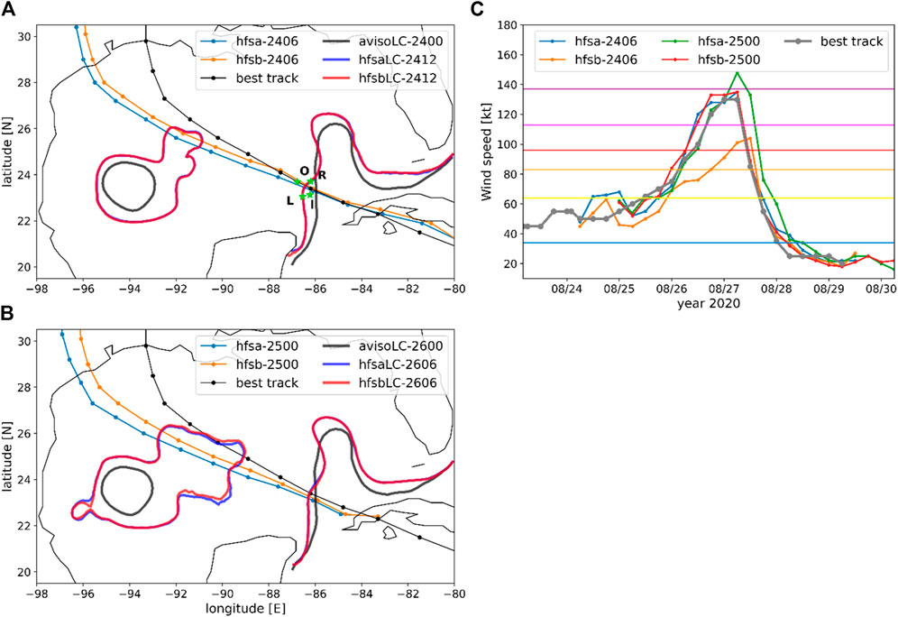
Figure 5. Comparisons of predicted tracks between HFSA (blue) and HFSB (orange) for the (A) 202082406 and (B) 2020082500 cycles superimposed on the best track (black); (C) Vmax intensities for both cycles and runs with respect to the observed intensity (best track). The blue/red curves in (A, B) denote 17 cm of sea-surface height anomalies (SSHAs) for HFSA/HFSB estimated at 06Z on 24/26 August 2020 (blue/red). The black curve represents the AVISO daily SSHAs at 00Z on (A) August 24 and (B) August 26. The four green stars denote the locations for the heat budget analysis (details in Section 4.2).

The HAFSv1 systematically shows a westward bias in the track forecasts, particularly for the later lifecycle of hurricane Laura. Nevertheless, we chose two cycles (2020082406 and 2020082500) for detailed analyses. The track forecasts are similar for both cycles and have mean absolute errors of ∼12.4 km and 28.7 km for cycles 2020082406 and 2020082500, respectively, compared to the best track (BT) (Figure 5). The track forecast errors increase gradually, and the maximum deviations from BT are ∼293.4/266.3 km for HFSA/HFSB for the former case and ∼357.8/279.5 km for the latter case. However, the intensity forecasts were quite different between the cycles, especially for the HFSB, which significantly underpredicted Vmax and also RI for the cycle 2020082406.

The observed TC had two RI events: a 25-kt Vmax change between 18Z on August 24 and 00Z on August 26 as the storm passed over the LC, and a 55-kt increase over 24 h from 00Z on August 26 to 00Z on August 27. The HFSA predicted one RI from 52 kt at 06Z on August 25 to 135 kt at 06Z on August 27; the HFSB showed RI in two phases, similar to the above observations, where both events started with underpredicted Vmax that first gained 23 kt over 24 h between 00Z on August 25 and 00Z on August 26, followed by another gains of 26 kt from 06Z on August 25 to 06Z on August 27.

3.1.2 Ocean observational data

The in situ Argo profiles and glider data were sourced from the World Ocean Database 18 (WOD18) and Coriolis database (http://www.coriolis.eu.org; Cabanes et al., 2013), respectively. The in situ SST observations were obtained from the US National Data Buoy Center (NDBC) database.

3.2 Methodology

3.2.1 Ocean variables and skill metrics

Each cycle simulation encompasses 6-hourly 3D volume outputs over a 126-h forecast period. The simulation assessments were focused on five ocean metrics, namely SST, mixed layer depth (MLD), mixed layer temperature (MLT), mixed layer salinity (MLS), and mean temperature over a 100-m depth (T100), as well as the OHC relative to the 26°C isotherm (Z26) as given by Eq. 1:

$OHC=C_p{\displaystyle {\int }_{z=0}^{z26}}{\rho }_z\left[T_z-26\right]\delta z,(1)$

where $C_p$ is the constant heat capacity of seawater (3,985 J kg⁻¹ K⁻¹), ${\rho }_z$ is the seawater density (kg m⁻³), and $T_z$ is the temperature (Celsius) at a depth of $z$ (Leipper and Volgenau, 1972). The MLD is defined as the minimum density jump of 0.0125 kg m^–3 or an equivalent temperature jump of 0.3°C across the base of a mixed layer and is one of the HYCOM diagnostic variables. These variables have a cause-and-effect relation for the ocean–TC coevolution and quantitatively indicate the heat loss due to direct SST cooling, vertical mixing, and advection by a TC. More details on these parameters may be found in Aristizábal Vargas et al. (2024).

The ocean validation was conducted with observations using the skill metrics of bias, root mean-squared error (RMSE), centered root mean-squared deviation (CRMSD), and Pearson correlation coefficient (CC), which are respectively expressed by Eqs. (2–5). Detailed explanations of these skill metrics may be found in Rochford (2016). A Python package supporting these metrics may be found at http://github.com/PeterRochford/SkillMetrics.

$bias=\frac{1}{n}{\displaystyle {\sum }_{i=1}^n}\left(y_i-x_i\right),(2)$

$RMSE=\sqrt{\frac{1}{n}{\displaystyle {\sum }_{i=1}^n}{\left(y_i-x_i\right)}^2},(3)$

$CRMSD=\sqrt{\frac{1}{n}{\displaystyle {\sum }_{i=1}^n}{\left[\right.\left(y_i-\underset{\_}{y}\right)-\left.\left(x_i-\underset{\_}{x}\right)\right]}^2},(4)$

and

$CC=\frac{{\displaystyle {\sum }_{i=1}^n}\left(y_i-\underset{\_}{y}\right)\left(x_i-\underset{\_}{x}\right)}{\sqrt{{\displaystyle {\sum }_{i=1}^n}{\left(y_i-\underset{\_}{y}\right)}^2{\displaystyle {\sum }_{i=1}^n}{\left(x_i-\underset{\_}{x}\right)}^2}},(5)$

where $y$ is the predicted and $x$ is the observed variable, and $n$ is the number of samples. The underbar represents the temporal mean of a variable over a 120-h forecast period.

To effectively visualize the skills of the models, we employed the normalized Taylor diagram (Taylor, 2001) on the essential ocean variables. The variables were first estimated from observations before being mapped to the model’s vertical layer, and comparisons were performed with the model counterparts through the nearest grid point and time at 6-h intervals for the upper 350-m depth.

3.2.2 Heat budget in the mixed layer

To assess the processes governing the bulk temperature in the upper layer in response to the TC, we used the heat budget expression for the mixed layer employed in the study on Hurricane Gilbert (Jacob et al., 2000):

$\frac{\partial T}{\partial t}=-\underset{Adv}{\underbrace{\left(u\frac{\partial T}{\partial x}+v\frac{\partial T}{\partial y}\right)}}-\underset{Qo}{\underbrace{\frac{Q_o}{{\rho }_0{C}_p{h}_m}}}-\underset{We}{\underbrace{\frac{w_e∆T}{h_m}}}-\alpha ,(6)$

where T is the bulk MLT, (u,v) are the current velocities at the MLD, $Q_o$ is the thermal energy flux, ${\rho }_0$ is the density of seawater (1,025 kg m^–3), $C_p$ is the heat capacity of seawater (3,850 J kg⁻¹ K⁻¹), $h_m$ is the MLD, $∆T$ is the temperature difference between the mixed layer base and MLT beneath, $w_e$ is the entrainment velocity at the base of the mixed layer, and $\alpha$ is the residual accounting for the heat storage controlled by the combination of air–sea exchange and turbulent diffusion.

The parameter $w_e$ is also the entrainment heat flux by vertical mixing across the base of the mixed layer and can be estimated the mass conservation equation (Jacob et al., 2000):

$w_e=\frac{\partial h_m}{\partial t}+u\frac{\partial h_m}{\partial x}+v\frac{\partial h_m}{\partial y}+w_m,(7)$

where $w_m$ is the vertical advection at $h_m$. The terms on the right-hand side (RHS) are diagnosed from the model output. In the HYCOM, the turbulent vertical (Kv) and horizontal diffusivity (Kd) are scale-dependent, with background values of 1 cm² s⁻¹ and 0.1 cm² s⁻¹, respectively.

The heat flux term on the RHS of Eq. 6 is estimated as the sum of the net radiative, latent heat, and sensible heat fluxes as received through CMEPS from the FV3 model at each coupling step (360 s).

4 Results

4.1 Comparisons with observed data

The normalized Taylor diagram for cycle 2020082406 (Figure 7A) shows that HFSA and HFSB have the best skill for T100, with CC of O(0.96) and CRMSD of ∼0.68°C. On the other hand, these models have the worst forecast skills for MLD, followed by SST. Between the HFSA and HFSB, the former has a slightly higher/lower skill for MLD/SST than the latter. According to the mean bias (Table 1), both HFSA and HFSB underperform for SST and MLD at O(1°C) and O(10–12 m), respectively, which are statistically significant at the 95% confidence level. The same negative bias for the modeled MLT and OHC shown in Table 1 suggests that HYCOM has poor skill in predicting the thermal state variables. However, the CC and CRMSD indicate that HYCOM has relatively good skill for predicting variations of the integrated properties, such as the OHC, T100, MLT, and MLS.

Table 1

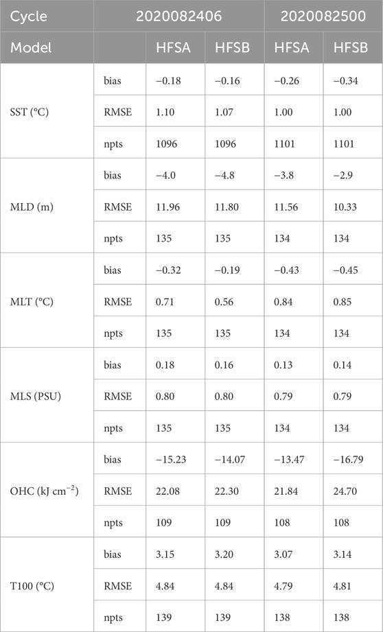
Table 1. Mean bias and RMSE for the SST, MLD, MLT, MLS, OHC, and T100 for the 2020082406 and 202082500 cycles. npts indicates number of points in counts.

Lower negative bias and RMSE, as shown in Table 1, considered together with the skill metrics shown in Figure 7A suggest that the upper layer simulations forced by the weaker Vmax of HFSB are in better agreement with the observations than those of the HFSA. For a similar and high Vmax (Figure 7B), however, HYCOM has poor skills, especially for the MLD, MLT, and OHC. Among these, MLD has the largest degradation, with CC values lower by ∼49%/58% and CRMSD higher by ∼18%/17% for the HFSA/HFSB. Interestingly, for similar Vmax forcing, the HYCOM coupled to HFSB exhibits higher skill deficit. The more negative biases for SST, MLT, and OHC in Table 1 for the 2020082500 case also support the observation of poor skills, specifically that HYCOM predicts a cooler upper ocean. As far as the CC, CRMSD, and standard deviation are concerned (Figure 7B), the only ocean metric that is improved for the 2020082500 case compared to the 2020082406 is the SST, implying that the HYCOM’s temporal and spatial SST variations are better predicted for stronger winds. It is noted that there are slight changes in the MLS skill, with CC of 0.81–0.82 and CRMSD of about 0.77–0.78, and small differences in the mean biases in the range of 0.13–0.18 PSU. In summary, high atmospheric winds impact the thermal properties and result in cooler conditions, and HYCOM has better forecast skills for wind with weaker Vmax values.

Figure 8 shows SST comparisons between the model and observations from the NDBC moorings for lead times of 60 h/42 h for the 2020082406 (b-e)/2020082500 (f-i) cycles. At 12Z on August 26, hurricane Laura was at (−91.4^oE, 26.4^oN), with 100-kt winds. The observations then ranged between 27.9°C and 32.8°C (Figure 8A). The minimum modeled SST from the 2020082406 cycle is ∼28.0°C, and the maximum SST is 31.9°C/32.3°C for HFSA (Figure 8D)/HFSB (Figure 8E). Figures 8H, I suggest that the model SSTs are generally higher along the northern and western coasts, with maximum values of 2.8/2.9°C for HFSA (Figure 8H)/HFSB (Figure 8I); this trend is opposite along the west and east coasts of Florida, with values of −3.0/−2.7°C for HFSA/HFSB. The mean bias is negative, and the values of the lead time are 0.34°C for HFSA and 0.32°C for HFSB. The model SST differences between the two configurations varied between −0.52°C and 0.32°C, with an average difference of −0.04°C (Figure 8B).

The modeled SST difference for the 2020082500 cycle is overall positive, ranging from −0.15°C to 0.49°C with a mean value of 0.06°C (Figure 8C). This probably resulted from less underprediction or smaller error by the HFSA (Figure 8J) than HFSB (Figure 8K). The mean SST error for HFSA is −0.29°C, with the values varying between −2.7 and 2.6°C, which is about 0.06°C smaller uncertainty compared to the HFSB counterpart.

At the time the storm was located ∼55.35 km west, a mooring at (−90.85^oE, 26.41^oN) observed an SST of 29.1°C. This suggests that the observed SST cooling by hurricane Laura was about 1.4°C. The observations also indicate that the SST cooling continued to decrease until it reached a local peak of O(28.3°C) at 18Z on August 26 and remained thus for at least 60 h thereafter. However, unfortunately, we cannot verify the magnitude of the storm-induced SST cooling from our simulations because of the bias in the predicted track, e.g., between 109.16 and 156.27 km to the southwest from the mooring location. Despite the bias, our estimates suggest similar degrees of SST cooling at the mooring site (1.75/1.32°C for HFSA/HFS for the 2020082406 cycle and 1.15/1.60°C for HFSA/HFSB for the 2020082500 cycle) and that the cooler SSTs remained consistent with the observed values until the end of the simulations.

Figure 10 shows the in situ T/S profile observations at 06Z on 26 August 2020. We chose this time to demonstrate the upper ocean conditions from the point observations during the intensification period. Since the simulations at these locations show little differences between the two forcing configurations, we only compare the HFSB simulations. Figure 10 suggests that HYCOM underestimates T and S in the upper mixed layer, which are reflected in the MLT, MLS, and MLD in Figure 7 and Table 1. We note that the T and S discrepancies become larger with depths, specifically toward cooler and fresher locations. At Argo 3 (Figure 10C), there were little changes in the upper T and S from the previous 10 days; this could be a part of the LC system and describes the condition 24 h after the passage of hurricane Laura. However, the 2020082500 cycle simulations depicts a deeper, cooler, and salty upper layer MLD (lighter blue and red) than the forecast from the 2020082406 cycle (darker blue and red), which might be due to the stronger and larger TC prediction. The HFSB predicts a large MLS at Argo 1 (Figure 10A) between the two cycles, with smaller errors for the 30-h forecasts of the 2020082500 cycle. Argo 2 exhibits strong stability at its location (Figure 10B), which may be caused by the deepening of the halocline over the previous 9.75 days. We found that HYCOM predicted this similarly. At the Argo 1 and 2 locations, the upper layer S below MLD was rather complex, yet HYCOM appeared to have difficulty in replicating reality, except that it was only able to provide rough estimates of the subsurface maximum S and depth.

A glider (4802976) situated at −90.98^oE and 26.54°N (g1 in Figure 6) encountered hurricane Laura at 12Z on August 26 about 44.5 km to the west. Figure 11 presents the time evolution of the upper T responses from the glider (a), HFSA and HFSB simulations (b–e), and the differences (f–i). When hurricane Laura approached the location, the upper layer responses included higher MLD and cooling MLT (Figure 11A). After hurricane Laura passed, the MLT continued cooling in an undulating pattern, with local extrema of 29.3 and 28.2°C, which was equivalent to about 1.3–2.4°C of cooling. The observed undulations that penetrated the depths were likely internal waves excited by the storm at the MLD base, and the largest amplitude of these motions was centered at a depth of ∼220 m. Unlike the observations, the HFSA (Figure 11B) and HFSB (Figure 11C) simulations are less impressive, especially for the post-storm period. Although HYCOM was able to simulate the cooling at a similar magnitude (Figures 11F, G), it failed to simulate the upwelling and undulating motions at least in the upper 130 m by either overpredicting or underpredicting Vmax for the 2020082406 case.

Figure 6

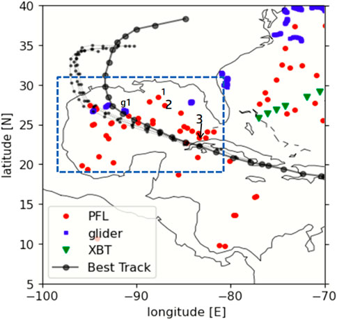
Figure 6. Locations of the temperature and salinity profiles from the Argo floats (PFL), gliders, and XBT as superimposed on the best track for the period from August 24 to August 30. Observations inside the dashed blue box are used in the study. The numbers in the box denote the locations of Argo 4903254, 4093238, and 4903252 for 1, 2, and 3, respectively; g1 is the location of glider 4802976.

The HFSA simulations for the 2020082500 cycle are not significantly different from the HFSB case (Figures 11D–I). However, one of the notable differences is less cooling at an average of 0.5°C, which could be due to smaller immediate cooling or warmer MLT resulting from the 23 kt difference in Vmax at the time that hurricane Laura passed (Figures 11F, H). Under HFSB forcing, the pre-storm conditions and MLT are similar to those of HFSA; however, the storm response is significantly different at least in the upper mixed layer (e.g., MLT cooling and its periodic variations). The temperature differences in the upper MLD suggest that the HFSB simulations best agree with the observations (Figure 11I), except for the overestimated MLT when hurricane Laura was situated closest.

Figures 11F–I suggest that a large temperature difference caused by the storm exists near the MLD base. We investigate this through the buoyancy frequency (N²). Figure 12 shows the mean N² before (black curve) and after hurricane Laura (red curve) from the glider observations (light curves with dots) based on interpolation at 2-m intervals from depths of 2–300 m over 3 hours from approximately 1.5–1.6 h samplings. There are two local peaks in the mean profile at 26 m and 65 m, with magnitudes of ∼55.0 × 10⁻⁵ s⁻². After hurricane Laura passed, both peaks moved to depths of 70–80 m, with 1.2–1.4 times increase in their magnitudes. The HFSA and HFSB pre-storm estimates showed two peaks as well, but their magnitudes were 1.3–1.4 times larger than those observed. The post-storm simulations exhibit one major peak in the mean N² for both the 2020082406 and 2020082500 cycles. Although these peaks exist at the same depth as in the observations, their values are as small or as large as 93.1 × 10⁻⁵ s^–2 or equivalently ∼1.5 to 1.7 times larger. The total number of glider profiles considered for the estimate is only 33, and their values are only 3.2 times those of the model profiles. These high variations in the observations are attributed to the fine vertical samplings, which governs the large N² value that is greater than 100 and less than 205 × 10⁻⁵ s⁻².

4.2 Mixed layer heat budget

Mesoscale features such as the cold/warm core eddies play a role in the TC intensification (Wang et al., 2018; Jaimes and Shay, 2015; Hong et al., 2000), which are explained by the SST feedback that primarily account for the vertical mixing in the oceanic upper layer. The objective here is to study the feedback associated with the oceanic thermal front, such as the LC, using the heat budget in the mixed layer. For detailed analyses, we chose four locations in the vicinity of the LC (see Figure 5A), each of which represents the individual TC quadrants. These are located at distances of 82.21–86.45 km between R34 and R50 from the TC center of the 30-h forecast for the 2020082406 case.

The heat tendency over the first 18 h (Figures 13A–D) changes abruptly from the maximum value O(<3.5°C d⁻¹) to a local minimum within a 3-h interval, as was common at all locations of interest. The first positive peak at 12 h is equally dominated by the heat flux (Figures 13I–L) and vertical entrainment (Figures 13M–Q) (see Table 2 for the extreme values that are omitted from Figure 13). Their cause may be explained by the thin MLD during the local daytime in contrast to the large solar heating.

Table 2

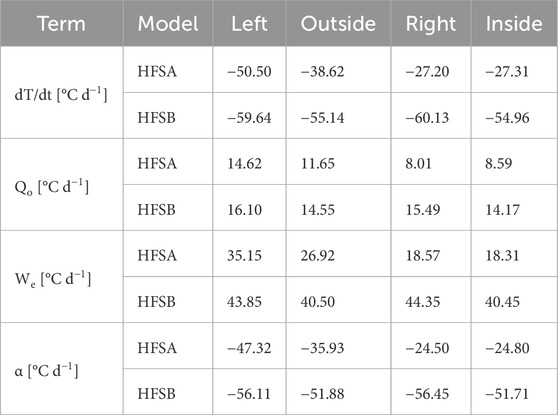
Table 2. Extreme values of the graphs not shown in Figure 13.

The tendency for the following 36 h varies at different locations. A point on the left side of the predicted track (Figure 13I) recovers heat from the local peak loss at 18 h (−2.55/−2.56 °C d⁻¹ for HFSA/HFSB) owing to the northward ocean currents that carry the warm Caribbean waters (positive advective term; Figure 13E). However, as hurricane Laura leaves, this point encounters the northerly and loses the acquired heat, reaching a local minimum peak that is as large as the first negative value. This is a result of the negative advection (Figures 13E) that brings relatively cooler water from the north, combined with the contributions from the surface heat flux (Figures 13I). Compared to the HFSB estimates (red in Figure 13A and orange in Figures 13E, I, M), we found relatively less negative advection (Figure 13E) and higher negative advection in the vertical direction (Figure 13M) that resulted in less negative heat in the mixed layer for the HFSA. However, the net values from the HFSA reversed over the next 6 h mainly because of delayed recovery of the northward currents, which was attributed to the relatively larger TC (∼1.18 times for the 30-h R34).

Compared to Figure 13I, the heat budget for the pre-storm period at a point outside the LC (Figures 13II) is lower and exhibits a notable difference between the HFSA and HFSB (Figure 13B), with the magnitude variation being ∼30% less for the former (blue) than the latter (orange). We found that this location exhibited the largest storm impact. The process responsible for the difference was the large entrainment for HFSB ($\le$−2.90°C d⁻¹) compared to that for HFSA (−1.61°C d⁻¹), which was caused by the relatively larger MLD horizontal (second and third terms on the RHS of Eq. 7) and vertical advections (fourth term on the RHS of Eq. 7) as well as larger temporal MLD changes (first term on the RHS of Eq. 7). The post-storm variations are larger for the HFSA than HFSB, which are dominated by advection (Figure 13G) and vertical entrainment (Figure 13Q). It is noted that all three source terms vary in time over a 24-h period but lag from each other by approximately 6 h.

At a point in the right quadrant (Figure 13III) where the MLD currents are mainly eastward, the storm and current interactions are a little more complicated than at other locations. For example, the advection source term (Figure 13G) shows the largest positive value for both models, with a larger magnitude (∼3.30/3.05°C d⁻¹) for HFSA than HFSB (2.21/2.37°C d⁻¹) at 36/54 h. Unlike Figure 13II, the variations of all the source terms are in phase, except for the in-storm period where the entrainment achieves a local maximum at 24 h and advection becomes almost zero (Figure 13G), in contrast to the local minimum of the entrainment and positive advection over the same period. While the heat flux term (Figure 13K) varies by only 0.09°C d⁻¹ from the mean values of −0.31°C d⁻¹ and −0.29°C d⁻¹ for the HFSA and HFSB, respectively, over the 36-h period from 18 to 54 h, the large heat advection (Figures 13G) overwhelms the sum of the negative heat flux (Figure 13K) and entrainment (Figure 13O). However, because of the large positive heat from advection and negative vertical entrainment, the net heat loss is longer by 6 h in the right quadrant. The major factor contributing to the peak at 36 h is the MLD current amplified by the tail end of the TC winds, but the second positive peak at 60 h is mainly caused by the MLT associated with the cold wake that extends upstream. It is found that the positive peaks of the entrainment at 48 h for the HFSA and 54 h for the HFSB are caused by MLD deepening via storm-induced mixing. However, the respective negative and positive peaks at 72 h and 84 h are caused by the cold wake from the undulation motions in the MLD.

A point inside the LC (Figure 13IV) exhibits the least variation among all source terms (Figures 13H, L, Q). However, because of the relatively long period of heat loss in the entrainment term (Figure 13Q) and heat flux with little variations (Figure 13L), the net heat budget was relatively constant during the transit of hurricane Laura (Figure 13D). In particular, the heat advection is small because of the relatively weak currents and uniform MLT inside the LC. Although the variations of the entrainment heat flux are small, the in-storm estimates definitely exhibit the influence of the storm, especially for HFSA whose predicted TC is stronger (by 5/10 kt at 30/36 h) and larger (by ∼1.18/1.16 times at 30/36 h for R34) than that by the HFSB. The RHS estimates (thin curves in Figures 13I–IV) explicitly demonstrate the heat changes before and after the 30-h forecast, which are associated with interactions with the front and rear quadrants, respectively.

It is of interest to observe the lag changes in the residual $\alpha$ (thin curves in Figures 13Q–T) before and after hurricane Laura. The post-storm $\alpha$ varies at a certain frequency but lags the heat tendency. On the other hand, the pre-storm estimates generally lead the tendency, and the lag time is shorter on the outside (Figure 13R) and inside (Figure 13T) than at the left (Figure 13Q) and right quadrants (Figure 13S). We can probably conclude that the governing processes for the lag difference is due to the shear instability driven by the TC winds, as opposed to buoyancy stability in response to the diurnal heat flux rather than mechanical wind forcing. We can also conclude that a relatively larger residual exists for the in-storm period and that the spatial variations are complex because of the non-linear interactions with the LC and TC.

5 Summary and conclusion

The GOM is a unique, semi-enclosed ocean where a TC can make a complete transit in as short as 2.5 days at an average speed of 5 m s⁻¹; further, it is one of the areas that are densely populated by TC activities, where storms can potentially experience rapid changes in intensity owing to the warm upper layers and various oceanic mesoscale features, such as the warm LC, cold/warm core eddies, and freshwater barrier that is often offshore advected from the Mississippi river discharge (Da Silva and Castelao, 2018). These features play crucial roles in the air–sea interactions, particularly modulating the enthalpy flux and consequently changing the TC intensity under the right environmental conditions. At the same time, the ocean responds to such changes, resulting in continuous feedback.

We validated the upper layer simulations from the coupled HAFS runs for two cycles of hurricane Laura, where the Vmax intensities were significantly underestimated for the 2020082406 and 2020082500 cycles. By examining the ocean variable such as SST, MLD, MLT, MLS, T100, and OHC, we obtained surprising findings regardless of the substantial differences in the predicted intensity forecasts. The skill assessments (Figure 7) suggest that underpredicted intensity forcing represents the ocean conditions better than high wind forcing. However, comparisons of the hydrographic profiles (Figure 10) showed no notable differences between the configurations of each cycle. Further, there were differences between the two cases, with degradation for HFSB over HFSA. This was primarily governed by the MLD (also shown in Figure 7), which is in turn associated with the MLT.

Figure 7

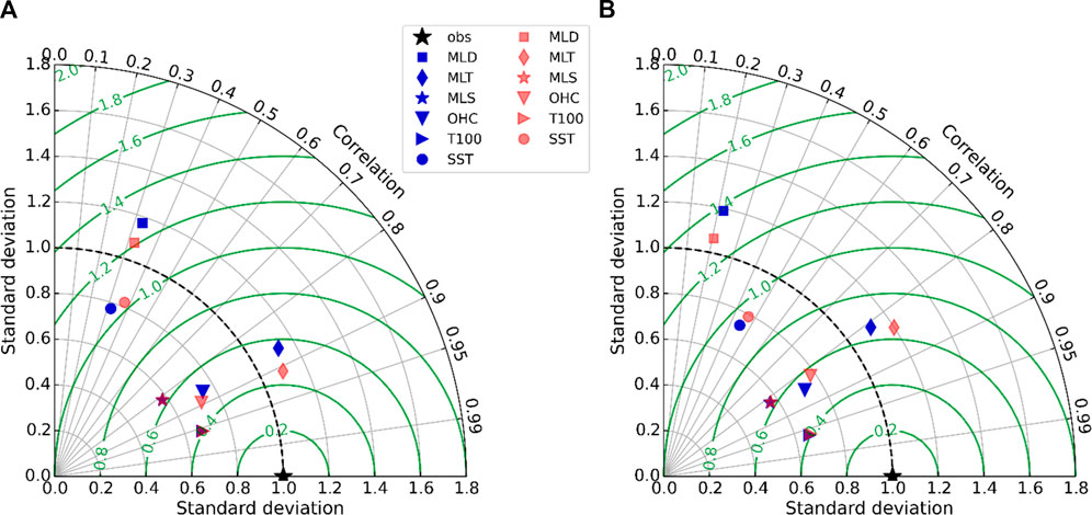
Figure 7. Skill comparisons via Taylor diagram for the (A) 202082406 and (B) 2020082500 cycles for mixed layer depth (MLD), mixed layer temperature (MLT), mixed layer salinity (MLS), ocean heat content (OHC), and mean temperature over 100-m depth (T100). The green contours represent the CRMSD.

The SST underperformed similar to the MLD. Comparisons with the NDBC mooring observations (Figure 8) demonstrated negative biases (−0.34°C to 0.16°C) with large variations in the range of −3.0°C to 2.9°C at the time of the peak winds (at 60-h and 42-h lead times for cycles 2020082406 and 20200825, respectively) that provide evidence supporting the skills. An SST value beneath the TC implies negative SST, meaning that there is higher cooling than that observed, and the cooling is greater for the HFSA in the 2020092406 case and HFSB in the 2020082500 case. Regardless of underpredicted or overpredicted intensity, the ocean simulations forced by the HFSB winds generally estimate warmer SSTs by an average of 0.5°C or 0.15°C (Figures 8B, C).

Figure 8

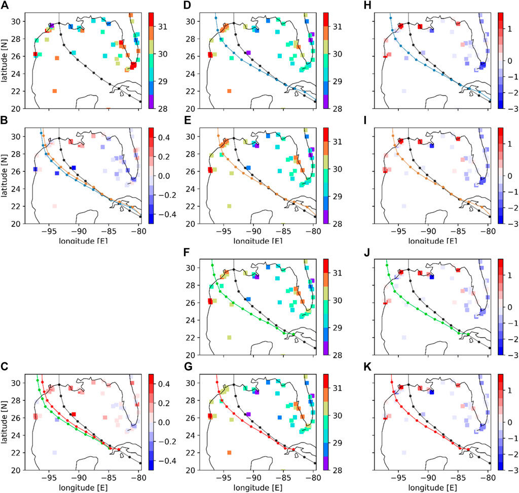
Figure 8. Comparisons of the SST at 12Z on August 26 at 52 NDBC mooring locations: (A) observations, (B–C) SST differences between HFSA and HFSB for the 20200824006 and 2020082500 cycles, respectively, (D–G) model SSTs for 60-h and 42-h lead times for cycles 2020082406 and 2020082500; (H–K) SST differences between the model and observations for the same lead forecast times for each cycle. The best and predicted tracks are shown by the black and colored curves with dots (ref. Figures 5A, B). The units are in degrees Celsius (°C).

Using the six-hourly model outputs, we quantified the magnitudes and variations of the upper layer responses in space and time between the two systems. Figure 9 shows the SST and MLD changes for the 202082406 case as an example. The upper ocean appears to respond proportionally to the forcing; for example, at the 60-h lead time, the estimated SST cooling is 2.9°C–4.1°C and the MLD deepens by about 47–57 m/34 m for the 76 kt/120 kt winds of the retrospective HFSB and HFSA, respectively. The figure also shows manifestation of inertial waves during the intensification period in an area between 1,000 and 1,600 km, which is weaker for weaker winds. The SST cooling variations associated with the inertial motions are similar for the HFSA and HFSB, but the mean bias is larger by 0.7°C for the latter. The MLD variations of the HFSB (Figure 9D) are 1.0/1.6 times that of the HFSA deepening/shoaling (Figure 9C) and indicate that there are two regimes dominated by shoaling and deepening across 1,300 km.

Figure 9

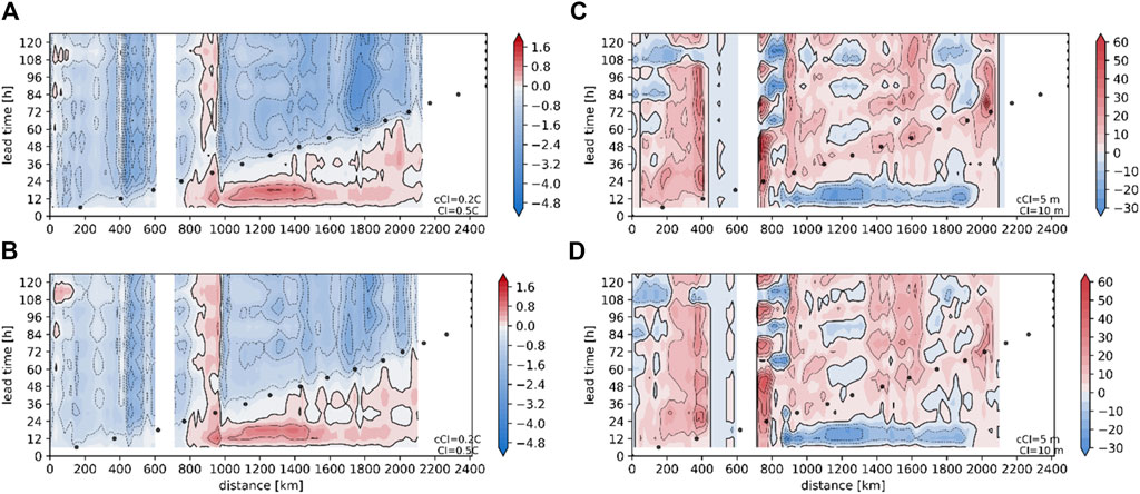
Figure 9. (A, B) SST and (C, D) MLD changes from the initial values as functions of the predicted tracks from the initial storm center (in km along x axis) and lead time (in hour along y axis) for hurricane Laura’s 2020082406 cycle for the (A, B) HFSA and (C, D) HFSB. Each black dot denotes the predicted storm center at the corresponding lead time (y axis) and location (x axis). The area between 600 and 720 km denotes Cuba, and the area between ∼440 and 600 km represents the Gulf of Batabano (model depth of 5 m).

Another response noted in Figure 9 is in the LC frontal region (at ∼950 km), where the SST response to the storm is drastically different between the windward side (inside the LC) and leeward side (outside the LC). Inside the LC, the storm induces warmer SSTs for the HFSA (Figure 9A) by about 0.2°C magnitude, but the opposite occurs outside the LC at a similar magnitude. A similar bimodal pattern exists for the HFSB (Figure 9B); however, the positive SST change in the windward side is about 0.2°C higher on average than that for the HFSA. The SST cooling outside the LC, on the other hand, is smaller by O($\le$0.15°C) than the HFSA counterpart. The MLD change in the same frontal area is not as drastic as the SST change, especially for the HFSB (Figure 9D); instead, there is a persistent deepening of the MLD in the windward side, with the magnitude varying in an undulation pattern. Hence, high Vmax prediction by the HFSA results in higher SST cooling (maximum of 3.5°C) and greater MLD deepening (maximum of 56.6 m) of 0.6°C and 10 m, respectively, than by the HFSB.

In comparison, the SST and MLD changes at a point in the right quadrant (∼50 km east of the TC center) estimate higher cooling by 0.7/0.2°C and shoaling by 11.9/4.1 m for the HFSA/HFSB, respectively, than those at the TC center (Figure 9). The local maximum of the positive SST change exists at the LC front again, whose magnitude is 0.6/0.8°C for the HFSA/HFSB. Compared to the SST changes in Figures 9A, B, the values are 3 and 1.6 orders of magnitude larger for the HFSA and HFSB, respectively, which are accounted for by the stronger wind stresses in the right quadrant. However, the lower MLD changes imply that the storm-induced upwellings are weaker than those at the predicted TC centers (Figure 9).

The location dependency of the storm coordinates is reflected in the heat budget as well. As seen in Figure 13, the budget in the upper mixed layer is less dramatic inside the LC (Figure 13IV) than that outside the LC (Figure 13II); this is because of the deep thermocline of the LC. However, the LC frontal area presents a more complex heat budget for storm interactions. The implicit processes investigated herein first include the non-linear interactions of the MLD currents with the cyclone winds that can be either interrupted or amplified. Second, the storm-induced vertical motions become significant. Third, local storm-induced cooling can be less significant because the advected heat would be the governing process.

Because of the heavy rains and thick clouds (Lin and Rossow, 1944; Karstens et al., 1994), remotely sensed SST observations using microwave sensors are minimally useful for SST validation. The gridded SST products are also less desirable because they are available at most daily, and the decorrelation length scale employed in the interpolation method (e.g., optimum Interpolation) may not adequately represent either the eddy-abundant real ocean conditions or rapid changes due to the fast-moving storm. Hence, validations were conducted using a few Argo profiles, dense but space-limited observations from gliders, and the NDBC moorings popular in shallow waters.

With the limited in situ observations, we found that the modeled T/S profiles agreed with the observations, especially in deep waters (Figures 10, 11). We also found similar SST cooling as the observations (Figure 8). However, we conclude that the HYCOM simulations are overall biased to the cold upper ocean conditions. The upper layer responses accordingly correspond to the winds, specifically the stronger winds, as well as larger SST and MLT biases. However, using the responses of the model MLD, such as the weaker winds, the higher MLD is difficult to explain using only the buoyancy frequency (Figure 12) without the shear instability.

Figure 10

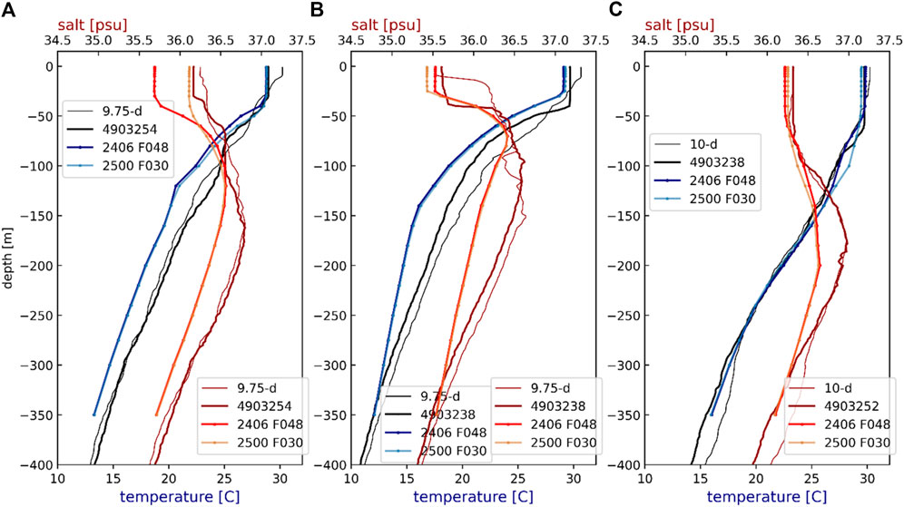
Figure 10. Temperature (T; thick black) and salinity (S; thick dark red) observations at 06Z (A–C) on 26 August 2020 at three locations (see Figure 6) compared with the modeled T (blue) and S (red) values for the HFSB at 48/30 h lead times for cycles 2020082406/2020082500. The T (think black) and S profiles (think dark red) sampled approximately (A, B) 9.75 days and (C) 10.0 days prior are also shown.

Figure 11

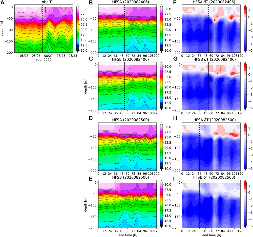
Figure 11. T transect along the glider 4802976 track (see Figure 6) (A) sampled at 6-h intervals and compared with (B, D) HFSA and (C, E) HFSB simulations for cycles 2020082406 and 2020082500 as functions of the lead time [h] along x axis and depth along y axis. The model T differences from observations shown for HFSA (F) and HFSB (G); and HFSA (H) and HFSB (I) for cycle 2020082406 and 2020082500, respectively. The units are in degrees Celsius. The closest distance to hurricane Laura is at 12Z on August 26 (dashed vertical lines at 54 h for cycle 2020092406 and 36 h for cycle 2020082500). The total excursion for the period is ∼47.2 km. The contour intervals are 0.5 °C for the shades and 1 °C for the contours.

Figure 12

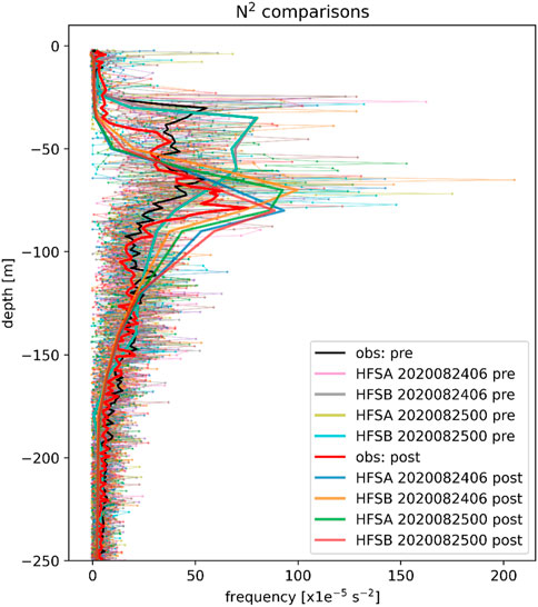
Figure 12. Mean buoyancy frequency (N²) for the pre- and post-storm periods for glider observations (black and red) superimposed on estimates from the individual observations (thin lines with dots). The model estimated profiles are shown for the period from before to after hurricane Laura for the 2020082406 and 2020082500 cycles. Note that the pre-storm mean profiles for each cycle are almost identical between the HFSA (light blue and orange for the 2020082406 and 2020082500 cycles, respectively) and HFSB (darker blue for cycle 2020082406 and green for cycle 2020082500).

We conducted heat budget investigations in the upper mixed layer in the LC area through HFSA and HFSB forcing. The results suggest that the heat balance is complex owing to the non-linear interactions between the oceanic thermal front and a TC (Figure 13). Inside the LC where the thermocline is deep, the storm impact on heat budget is mainly through advection and entrainment flux. However, the points in the LC front exhibit that the two advection and entrainment flux terms either counteract or enhance the heat depending on the storm quadrant. Specifically, the entrainment flux is significant enough to render the heat budget negative. The time series of the heat tendency (Figure 13) suggests that the perennial heat supply in the LC by the strong currents can be interrupted by the TC and that such a pause can be as long as 21 h. We found that there were relatively significant heat residuals, especially over the in-storm period. This was accounted for by the unresolved mixing in the shear-dominant environment. One way to rectify this is to at least include wave coupling to explicitly consider the Langmuir turbulence mixing as well as non-linear interactions with the waves, TC, and ocean currents.

Figure 13

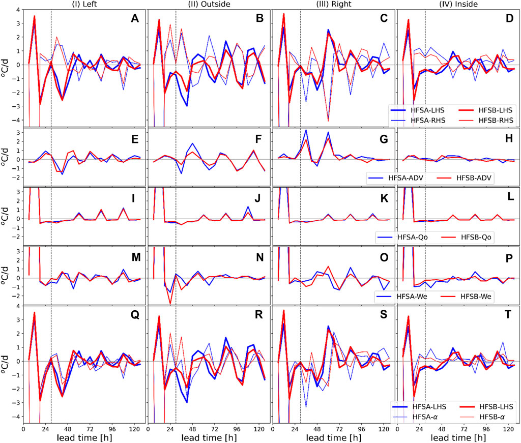
Figure 13. Time series of the heat budget estimates for the 2020082406 cycle at four points of interest (Figure 5A): (A–D) show the tendencies of the total heat in thick/thin blue and red lines for the left-hand side (LHS)/right-hand side (RHS) of Eq. 6; (E–H) depict the advection terms; (I–L) depict the heat flux terms; (M–P) are the entrainment terms on the RHS of Eq. 6; (Q–T) are the residuals $\alpha$ (thin blue and red lines) against the tendencies (thick lines). The light blue and orange lines in (E–P) denote the HFSA and HFSB estimates, respectively. The locations of the points are (−86.55^oE, 23.05^oN), (−86.78^oE, 23.69^oN), (−86.20^oE, 23.71^oN), and (−86.23^oE, 23.13^oN) for I–IV, respectively, where I and III are at the LC front and the others are outside (II) and inside (IV) the LC. See Table 2 for the extreme values omitted from each panel.

Data availability statement

The original contributions presented in the study are included in the article/Supplementary Material, and any further inquiries may be directed to the corresponding author.

Author contributions

H-SK: Conceptualization, Data curation, Formal analysis, Funding acquisition, Investigation, Methodology, Project administration, Resources, Software, Supervision, Validation, Visualization, Writing–original draft, Writing–review and editing. BL: Software, Validation, Writing–review and editing. BT: Software, Writing–review and editing. DR: Software, Writing–review and editing. WW: Methodology, Writing–review and editing. AH: Methodology, Writing–review and editing. ZZ: Resources, Supervision, Writing–review and editing. XZ: Resources, Supervision, Writing–review and editing. AM: Resources, Supervision, Writing–review and editing.

Funding

The authors declare that financial support was received for the research, authorship, and/or publication of this article. This project was funded by the NOAA Hurricane Improvement Program (HFIP).

Acknowledgments

This work would be not accomplished without contributions from the AOML and EMC scientists as well as support from the NOAA Hurricane Forecast Improvement Program (HFIP). HAFS is a multi-institutional collaborative work with partners from EMC, AOML, and GSL. The authors acknowledge the UFS development team for assistance with seamlessly merging HAFSv1 to the UFS framework. The water temperature data are provided by NOAA’s National Data Buoy Center (http://www.ndbc.noaa.gov). The Argo and glider profiles were obtained from the World Ocean Database 18 (WOD18) and Coriolis database (http://www.coriolis.eu.org; Cabanes et al., 2013). The altimetry data were produced by Salto/Duacs and distributed by AVISO, with support from the Centre National d’Etudes Spatiales.

Conflict of interest

The authors declare that the research was conducted in the absence of any commercial or financial relationships that could be construed as a potential conflict of interest.

Publisher’s note

All claims expressed in this article are solely those of the authors and do not necessarily represent those of their affiliated organizations or those of the publisher, editors, and reviewers. Any product that may be evaluated in this article or claim that may be made by its manufacturer is not guaranteed or endorsed by the publisher.

Supplementary material

The Supplementary Material for this article can be found online at: https://www.frontiersin.org/articles/10.3389/feart.2024.1399409/full#supplementary-material

References

Aristizábal Vargas, M. F., Kim, H. S., Le Hénaff, M., Miles, T., Glenn, S., and Goni, G. (2024). Evaluation of the ocean component on different coupled hurricane forecasting models using upper-ocean metrics relevant to air-sea heat fluxes during Hurricane Dorian (2019). Front. Earth Sci. 12. doi:10.3389/feart.2024.1342390

CrossRef Full Text | Google Scholar

Avila-Alonso, D., Baetens, J. M., Cardenas, R., and De Baets, B. (2020). Oceanic response to the consecutive hurricanes dorian and humberto (2019) in the sargasso sea. Nat. Hazards Earth Syst. Sci. Discuss. 2020, 1–29. doi:10.5194/nhess-21-837-2021

CrossRef Full Text | Google Scholar

Biswas, M. K., Sergio Abarca, A., Bernardet, L., Ginis, I., Grell, E., Iacono, M., et al. (2018). Hurricane weather research and forecasting (HWRF) model: 2018 scientific documentation november 2018.

Google Scholar

Bleck, R. (2002). An oceanic general circulation model framed in hybrid isopycnic-Cartesian coordinates. Ocean Modell. 4 (1), 55–88.

CrossRef Full Text | Google Scholar

Burnett, W., Harper, S., Preller, R., Jacobs, G., and LaCroix, K. (2014). Overview of operational ocean forecasting in the US Navy: past, present, and future. Oceanography 27 (3), 24–31. doi:10.5670/oceanog.2014.65

CrossRef Full Text | Google Scholar

Cabanes, C., Grouazel, A., von Schuckmann, K., Hamon, M., Turpin, V., Coatanoan, C., et al. (2013). The CORA dataset: validation and diagnostics of in-situ ocean temperature and salinity measurements. Ocean. Sience 9, 1–18. doi:10.5194/os-9-1-2013

CrossRef Full Text | Google Scholar

Chassignet, E. P., Hurlburt, H. E., Smedstad, O. M., Halliwell, G. R., Hogan, P. J., Wallcraft, A. J., et al. (2007). The HYCOM (hybrid coordinate ocean model) data assimilative system. J. Mar. Syst. 65 (1-4), 60–83. doi:10.1016/j.jmarsys.2005.09.016

CrossRef Full Text | Google Scholar

Chassignet, E. P., Yeager, S. G., Fox-Kemper, B., Bozec, A., Castruccio, F., Danabasoglu, G., et al. (2020). Impact of horizontal resolution on global ocean–sea ice model simulations based on the experimental protocols of the Ocean Model Intercomparison Project phase 2 (OMIP-2). Geosci. Model. Dev. 13 (9), 4595–4637. doi:10.5194/gmd-13-4595-2020

CrossRef Full Text | Google Scholar

Cummings, J. A. (2005). Operational multivariate ocean data assimilation. Quart. J. R. Metall. Soc. Part C 131 (613), 3583–3604. doi:10.1256/qj.05.105

CrossRef Full Text | Google Scholar

Cummings, J. A., and Smedstad, O. M. (2013). Variational data assimilation for the global ocean. Data Assim. Atmos. Ocean. hydrologic Appl. II, 303–343. doi:10.1007/978-3-642-35088-7_13

CrossRef Full Text | Google Scholar

Da Silva, C. E., and Castelao, R. M. (2018). Mississippi River plume variability in the Gulf of Mexico from SMAP and MODIS-Aqua observations. J. Geophys. Res. Oceans 123 (9), 6620–6638. doi:10.1029/2018jc014159

CrossRef Full Text | Google Scholar

Eley, E. N., Subrahmanyam, B., and Trott, C. B. (2021). Ocean–atmosphere interactions during hurricanes marco and Laura (2020). Remote Sens. 13 (10), 1932. doi:10.3390/rs13101932

CrossRef Full Text | Google Scholar

Garraffo, Z. D., Cummings, J. A., Paturi, S., Hao, Y., Iredell, D., Spindler, T., et al. (2020). “RTOFS-DA: real time ocean-sea ice coupled three dimensional variational global data assimilative ocean forecast system,” in Research activities in Earth system modelling. Editor E. Astakhova (China: WMO, World Climate Research Program Report No.6). (PDF, available here) July, 2020).

Google Scholar

Gong, Q., Wang, Q., Chen, L., Diao, Y., Xiong, X., Sun, J., et al. (2023). Observation of near-inertial waves in the wake of four typhoons in the northern South China Sea. Sci. Rep. 13 (1), 3147. doi:10.1038/s41598-023-29377-3

PubMed Abstract | CrossRef Full Text | Google Scholar

Halliwell, G. R. (2004). Evaluation of vertical coordinate and vertical mixing algorithms in the HYbrid-Coordinate Ocean Model (HYCOM). Ocean. Model. 7 (3-4), 285–322. doi:10.1016/j.ocemod.2003.10.002

CrossRef Full Text | Google Scholar

Heffner, D. M., Subrahmanyam, B., and Shriver, J. F. (2008). Indian Ocean Rossby waves detected in HYCOM sea surface salinity. Geophys. Res. Lett. 35 (3). doi:10.1029/2007gl032760

CrossRef Full Text | Google Scholar

Hong, X., Chang, S. W., Raman, S., Shay, L. K., and Hodur, R. (2000). The interaction between Hurricane Opal (1995) and a warm core ring in the Gulf of Mexico. Mon. Weather Rev. 128 (5), 1347–1365. doi:10.1175/1520-0493(2000)128<1347:tibhoa>2.0.co;2

CrossRef Full Text | Google Scholar

Jacob, S. D., Shay, L. K., Mariano, A. J., and Black, P. G. (2000). The 3D oceanic mixed layer response to Hurricane Gilbert. J. Phys. Oceanogr. 30 (6), 1407–1429. doi:10.1175/1520-0485(2000)030<1407:tomlrt>2.0.co;2

CrossRef Full Text | Google Scholar

Jaimes, B., and Shay, L. K. (2015). Enhanced wind-driven downwelling flow in warm oceanic eddy features during the intensification of Tropical Cyclone Isaac (2012): observations and theory. J. Phys. Oceanogr. 45 (6), 1667–1689. doi:10.1175/jpo-d-14-0176.1

CrossRef Full Text | Google Scholar

Kara, A. B., Helber, R. W., and Wallcraft, A. J. (2010). Evaluations of threshold and curvature mixed layer depths by various mixing schemes in the Mediterranean Sea. Ocean. Model. 34 (3-4), 166–184. doi:10.1016/j.ocemod.2010.05.006

CrossRef Full Text | Google Scholar

Kara, A. B., Wallcraft, A. J., and Hurlburt, H. E. (2005). Sea surface temperature sensitivity to water turbidity from simulations of the turbid Black Sea using HYCOM. J. Phys. Oceanogr. 35 (1), 33–54. doi:10.1175/jpo-2656.1

CrossRef Full Text | Google Scholar

Kara, A. B., Wallcraft, A. J., Martin, P. J., and Chassignet, E. P. (2008). Performance of mixed layer models in simulating SST in the equatorial Pacific Ocean. J. Geophys. Res. Oceans 113 (C2). doi:10.1029/2007jc004250

CrossRef Full Text | Google Scholar

Karstens, U., Simmer, C., and Ruprecht, E. (1994). Remote sensing of cloud liquid water. Meteorology Atmos. Phys. 54, 157–171. doi:10.1007/bf01030057

CrossRef Full Text | Google Scholar

Kim, H.-S., Lozano, C., Tallapragada, V., Iredell, D., Sheinin, D., Tolman, H. L., et al. (2014). Performance of ocean simulations in the coupled HWRF–HYCOM model. J. Atmos. Ocean. Technol. 31 (2), 545–559. doi:10.1175/jtech-d-13-00013.1

CrossRef Full Text | Google Scholar

Kim, H.-S., Meixner, J., ThomasReichl, B. G. B., Liu, B., Mehra, A., Wallcraft, A., et al. (2022). Skill assessment of NCEP three-way coupled HWRF–HYCOM–WW3 modeling system: hurricane Laura case study. Weather Forecast. 37 (8), 1309–1331. doi:10.1175/waf-d-21-0191.1

CrossRef Full Text | Google Scholar

Large, W. G., McWilliams, J. C., and Doney, S. C. (1994). Oceanic vertical mixing: a review and a model with a nonlocal boundary layer parameterization. Rev. Geophys. 32 (4), 363–403. doi:10.1029/94rg01872

CrossRef Full Text | Google Scholar

Leipper, D. F., and Volgenau, D. (1972). Hurricane heat potential of the Gulf of Mexico. J. Phys. Oceanogr. 2, 218–224. doi:10.1175/1520-0485(1972)002<0218:hhpotg>2.0.co;2

CrossRef Full Text | Google Scholar

Lin, B., and Rossow, W. B. (1994). Observations of cloud liquid water path over oceans: optical and microwave remote sensing methods. J. Geophys. Res. Atmos. 99 (D10), 20907–20927. doi:10.1029/94JD01831

CrossRef Full Text | Google Scholar

Lin, S.-J. (2004). A “vertically Lagrangian” finite-volume dynamical core for global models. Mon. Weather Rev. 132, 2293–2307. doi:10.1175/1520-0493(2004)132<2293:AVLFDC>2.0.CO;2

CrossRef Full Text | Google Scholar

Lin, S.-J., and Rood, R. B. (1996). Multidimensional flux-form semi-Lagrangian transport schemes. Mon. Weather Rev. 124, 2046–2070. doi:10.1175/1520-0493(1996)124<2046:MFFSLT>2.0.CO;2

CrossRef Full Text | Google Scholar

Marchok, T. (2021). Important factors in the tracking of tropical cyclones in operational models. J. Appl. Meteorol. Climatol. 60, 1265–1284. doi:10.1175/JAMC-D-20-0175.1

CrossRef Full Text | Google Scholar

Marler, M. (2023). FEMA's fumble: assessing the implications of inadequate long-term storm relief for Louisiana.

Google Scholar

Mehra, A., and Rivin, I. (2010). A real time ocean forecast system for the North Atlantic Ocean. TAO Terr. Atmos. Ocean. Sci. 21 (1), 211. doi:10.3319/tao.2009.04.16.01(iwnop)

CrossRef Full Text | Google Scholar

Metzger, E. J., Smedstad, O. M., Thoppil, P. G., Hurlburt, H. E., Cummings, J. A., Wallcraft, A. J., et al. (2014). US Navy operational global ocean and Arctic ice prediction systems. Oceanography 27 (3), 32–43. doi:10.5670/oceanog.2014.66

CrossRef Full Text | Google Scholar

Pasch, R., Berg, R., Roberts, D. P., and Papin, P. P. (2021). Hurricane Laura (AL132020). National hurricane center tropical cyclone report. Available at: https://www.nhc.noaa.gov/data/tcr/AL132020_Laura.pdf.

Google Scholar

Pottapinjara, V., and Joseph, S. (2022). Evaluation of mixing schemes in the HYbrid coordinate Ocean Model (HYCOM) in the tropical Indian ocean. Ocean. Dyn. 72 (5), 341–359. doi:10.1007/s10236-022-01510-2

CrossRef Full Text | Google Scholar

Purser, R. J., Jovic, D., Ketefian, G., Black, T., Beck, J., Dong, J., et al. (2020). The Extended Schmidt Gnomonic grid for regional applications. Available at: https://dtcenter.org/sites/default/files/events/2020/2-purser-james.pdf.

Google Scholar

Rasmussen, T. A., Kliem, N., and Kaas, E. (2011). The Effect of climate change on the sea ice and hydrography in Nares Strait. Atmosphere-Ocean 49 (3), 245–258. doi:10.1080/07055900.2011.604404

CrossRef Full Text | Google Scholar

Rochford, P. A. (2016). SkillMetrics: a Python package for calculating the skill of model predictions against observations. Available at: http://github.com/PeterRochford/SkillMetrics.

Google Scholar

Subrahmanyam, B., Heffner, D. M., Cromwell, D., and Shriver, J. F. (2009). Detection of Rossby waves in multi-parameters in multi-mission satellite observations and HYCOM simulations in the Indian Ocean. Remote Sens. Environ. 113 (6), 1293–1303. doi:10.1016/j.rse.2009.02.017

CrossRef Full Text | Google Scholar

Taylor, K. E. (2001). Summarizing multiple aspects of model performance in a single diagram. J. Geophys. Res. Atmos. 106 (D7), 7183–7192. doi:10.1029/2000jd900719

CrossRef Full Text | Google Scholar

Wang, A., Du, Y., Zhuang, W., and Qi, Y. (2015). Correlation between subsurface high-salinity water in the northern South China Sea and the North Equatorial Current–Kuroshio circulation system from HYCOM simulations. Ocean Sci. 11 (2), 305–312. doi:10.5194/os-11-305-2015

CrossRef Full Text | Google Scholar

Wang, G., Zhao, B., Qiao, F., and Zhao, C. (2018). Rapid intensification of Super Typhoon Haiyan: the important role of a warm-core ocean eddy. Ocean. Dyn. 68 (12), 1649–1661. doi:10.1007/s10236-018-1217-x

CrossRef Full Text | Google Scholar

Wang, W., Han, J. H., Shin, J., Chen, X., Hazelton, A., Zhu, L., et al. (2024). Physics schemes in the first version of NCEP operational hurricane analysis and forecast system (HAFS). Front. Earth Sci. 12. doi:10.3389/feart.2024.1379069

CrossRef Full Text | Google Scholar

Worthen, D., Wang, J., Monturo, R., Heinzeller, D., Li, B., Theurich, G., et al. (2024). Coupling infrastructure capability in U.S. Department of commerce, national oceanic and atmospheric administration. Natl. Weather Serv. Natl. Centers Environ. Predict. Submitt. doi:10.25923/dvv2-3g03

CrossRef Full Text | Google Scholar

Zamudio, L., and Hogan, P. J. (2008). Nesting the Gulf of Mexico in atlantic HYCOM: oceanographic processes generated by hurricane ivan. Ocean. Model. 21 (3-4), 106–125. doi:10.1016/j.ocemod.2007.12.002

CrossRef Full Text | Google Scholar

Zhang, Z., Wang, W., Doyle, J. D., Moskaitis, J., Komaromi, W. A., Heming, J., et al. (2023). A review of recent advances (2018-2021) on tropical cyclone intensity change from operational perspectives, Part 1: dynamical model guidance. Trop. Cyclone Res. Rev. 12 (1), 30–49. doi:10.1016/j.tcrr.2023.05.004

CrossRef Full Text | Google Scholar

Glossary