 Kun Gao
 Lucas Harris
 Mingjing Tong2
94% of researchers rate our articles as excellent or good
Learn more about the work of our research integrity team to safeguard the quality of each article we publish.
Find out more
ORIGINAL RESEARCH article
Front. Earth Sci. , 16 May 2024
Sec. Atmospheric Science
Volume 12 - 2024 | https://doi.org/10.3389/feart.2024.1396390
This article is part of the Research Topic Tropical Cyclone Modeling and Prediction: Advances in Model Development and Its Applications View all 13 articles
Tropical cyclone (TC) intensity forecasting poses challenges due to complex dynamical processes and data inadequacies during model initialization. This paper describes efforts to improve TC intensity prediction in the Geophysical Fluid Dynamics Laboratory (GFDL) System for High-resolution prediction on Earth-to-Local Domains (SHiELD) model by implementing a Vortex Initialization (VI) technique. The GFDL SHiELD model, relying on the Global Forecast System (GFS) analysis for initialization, faces deficiencies in initial TC structure and intensity. The VI method involves adjusting the TC vortex inherited from the GFS analysis and merging it back into the environment at the observed location, enhancing the analyzed representation of storm structure. We made modifications to the VI package implemented in the operational Hurricane Analysis and Forecast System, including handling initial condition data, reducing input domain size, and improving storm intensity enhancement. Experiments using the T-SHiELD configuration demonstrate that using VI significantly improves the representation of initial TC intensity and size, enhancing TC predictions, particularly in storm intensity and outer wind forecasts within the first 48 h.
Tropical cyclone (TC) intensity forecasts have been a persistent challenge, primarily attributed to the complex dynamical processes affecting the storm intensity changes and the inadequacy of data for model initialization in the inner core region. Predicting the intensity evolution of initially strong TCs is particularly difficult if the model depends on external datasets generated by a coarse-resolution model used for its initialization. In such cases, the storm structure and intensity are typically not adequately represented. A variety of vortex initialization (VI) methods have been proposed to improve the representation of the TC vortex in Numerical Weather Prediction models, which were well summarized by Liu et al. (2020).
The operational hurricane forecasting models at National Oceanic and Atmospheric Administration (e.g., Hurricane Analysis and Forecast System, or HAFS; Hurricane Weather Research and Forecasting model, or HWRF) commonly employ a combination of VI and data assimilation (DA) to create a proper three-dimensional initial storm structure that more accurately depicts the current state of the observed storm (Tong et al., 2018). VI here refers to a relatively simple technique for adjusting size and intensity of the TC vortex in the model initial state (see Section 2.1 for an overview). In the self-cycled operational hurricane models, VI is used to create the first guess for the DA system, which in turn, utilizes various observations to further refine the storm structure.
In research-oriented models, such as the Geophysical Fluid Dynamics Laboratory (GFDL) System for High-resolution prediction on Earth-to-Local Domains (SHiELD; Harris et al., 2020), VI or DA cycling is typically not used. The forecast jobs are usually cold started and launched independently. However, even in this setup, the model can still benefit from an improved storm initialization. The SHiELD applications usually relies on the Global Forecast System (GFS) analysis for model initialization. While this is generally valid for synoptic weather patterns, there can be notable deficiencies in the representation of initial TC structure and intensity due to the coarse resolution used by GFS. The use of the VI could be an effective means to improve the representation of initial TC vortex structure.
In this work, we adopt a similar VI approach as in HAFS and HWRF to adjust the initial TC vortex in GFDL SHiELD applications because of its simplicity and computational efficiency. This approach extracts the TC vortex in existing atmospheric state and adjust its size and intensity to match with observed values. Our main objectives are to document the change we made in the public-released VI package in HAFS, and also present our first attempt to use VI to improve TC forecasts in SHiELD applications.
The technical details of the VI method are well documented in Liu et al. (2020) and we only present a brief overview here of the basic ideas. First, the TC vortex and its surrounding environment components are separated following the vortex filtering method originally developed by Kurihara et al. (1995; K95 hereafter). The TC vortex component is then adjusted to ensure some of its characteristics (intensity, size parameters) match with the estimated values of the observed storm, while the environmental component remains untouched. As the last step, the adjusted TC vortex flow component is merged back into the environment, with its center relocated to the observed location. The operational dataset for observed TCs is the Tropical Cyclone Vitals Database (TC vitals), which is generated in real time by the National Hurricane Center.
The VI code package is structured into two layers. The lower layer consists the code that handles the actual VI tasks, such as vortex filtering, storm size and intensity adjustments, and vortex-environment merge. This layer of code requires input data adhering to a fixed format, which contains atmospheric variables in a storm-centered latitude-longitude box on A grids. The upper layer, which is the Input/Output (I/O) layer, is designed to perform two primary functions: a) formatting model-specific data to match the requirements of the lower layer, and b) post-processing the output of the lower layer into a format directly useable by the model.
In the operational models where the continuous DA cycling mode is used, VI is used as a procedure to create the first guess field for the DA system. The initial TC vortex could either be extracted from the GFS analysis, or the 6-h forecast from the previous cycle, depending on the availability of the previous forecast and the storm intensity. The extracted TC vortex will go through the VI steps (if the intensity is weaker than the observed value) and then be merged with the environmental component at the observed location.
We aim to adopt the same VI package used by HAFS (https://github.com/hafs-community/HAFS/tree/develop/sorc/hafs_tools.fd) to improve the TC initialization in SHiELD applications. During the development process, we made several modifications (described below) to facilitate the implementation of the package into the SHiELD workflow.
a) Introduced new capacity to handle the initial condition data created by SHiELD pre-processing package
In a cycled forecast system, the forecast initialized at a given time relies on the forecast from the previous cycle (e.g., the 06:00 UTC forecast job relies on the data produced by the 00:00 UTC job). However, for most SHiELD applications, cycling is not used. Instead, the SHiELD forecasts are usually cold-started and launched directly using the initial condition (IC) files generated by a pre-processing package. These IC files are in NetCDF format and have the same horizontal layout as the model grid (i.e., the cubed-sphere tiles).
We introduced new capacity to the VI package to handle SHiELD IC files, which involves introducing new code to the upper I/O layer as described in Section 2.1. We created new functionality that prepares the data in the required format for the lower layer based on IC files. Additionally, it post-processes the output of the lower layer into a format that is consistent with the original IC files. Specifically, our new functionality handles tasks such as i) transforming horizontal Earth-relative wind components between A grids and the staggered grids, ii) selecting data in a uniform latitude-longitude box centered at the TC center from the IC file, and iii) merging the selected boxed data (VI-adjusted) back to the IC file.
b) Reduced input domain size
The vortex filtering method developed by K95 contains two steps. In the first step, the total field is split into the basic field and disturbance field with an iteratively applied local filter (see equations 3.4–3.6 in Kurihara et al., 1993). In the second step, the disturbance field is further divided into the TC and non-TC disturbances through an optimum interpolation method as in K95.
To clarify the terminologies used thus far, the environment component we mentioned earlier constitutes the basic field and the non-TC disturbances (consistent with the terminologies used in K95 and Liu et al., 2020). In the second step of the K95 method, the filter domain is determined based on the tangential component of the total disturbance wind at a given level (e.g., 850 mb) along 24 radial directions. The filter domain therefore can have an irregular polygonal shape (see Figure 2A in K95).
In the current HAFS implementation, both steps of the filtering procedure operate on data that have been coarse-grained to 1° resolution over a 40 x 40° domain, centered on the storm. The high-resolution TC vortex for the subsequent size and intensity adjustment operations is obtained by subtracting the coarse-resolution environment component from the total high-resolution data.
The 40 x 40° data are generated by blending data from the high-resolution inner-nest and the coarser-resolution outer nest in HAFS. However, for SHiELD applications, certain storms may be positioned too close to the tile edges, hindering the selection of 40 x 40° boxed data. This holds true for both the parent global tile and the nested high-resolution tile.
We also noticed that in the HAFS implementation, the actual vortex filter domain determined via the K95 method undergoes additional smoothing along the azimuthal direction and then is further limited based on the observed Radius of the Outermost Closed Isobar (ROCI). The final filter domain is thus mostly circular, with its radius not exceeding 1.1 times of the ROCI in any of the 24 radial directions.
Due to the aforementioned reasons, we reduced the required domain size of the input data for the VI procedures from 40 x 40° to 10 x 10°. This change significantly relaxes the data requirement, allowing more TCs to qualify for VI even when their location is not too distant from the grid tile edges. While the change in domain size may not matter much for the detection of the filter domain, as it can always be contained in the 10 x 10° box, we acknowledge that it does affect the first step of the vortex filtering procedure due to the repeated application of the local filters. However, in practice, we observed that the impact of the domain size on the filtering results is overall insignificant, as shown in Figure 1.
c) Improved method for storm intensity enhancement
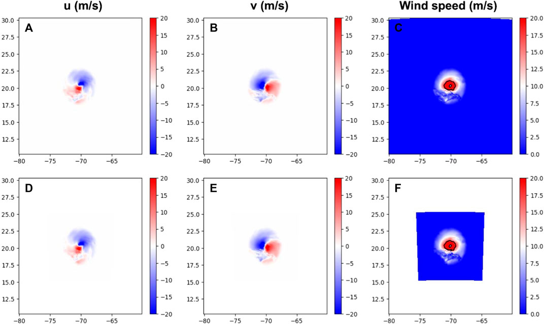
Figure 1. The tropical cyclone vortex obtained via the vortex filtering procedure based on data in a 40 x 40° latitude-longitude box (A–C) and 10 x 10° box (D–F). The 10 m height wind fields shown are from Hurricane Fiona (2022) and extracted from the GFS analysis on 2022-09-20 00:00 UTC. The left panel is the longitudinal wind, middle panel is the latitudinal wind, and the right panel is the total horizontal wind speed. The wind pattern to the south of the storm center was affected by the land surface.
In the current HAFS implementation, storm size and intensity adjustments are performed after the vortex filtering procedure, with technical details well described in Liu et al. (2020). Here we only describe our modification on the intensity enhancement strategy, which is only applied when the size-adjusted storm still has an intensity lower than the observed intensity (often true for hurricane-strength storms).
By default, the storm enhancement is done by adding a portion of an axisymmetric “bogus” vortex to the existing vortex. This “bogus” vortex can be either the azimuthally-averaged TC vortex from the 6-h forecast from the previous cycle, or a predefined axisymmetric synthetic vortex (Liu et al., 2020). In the present study, we use a predefined synthetic vortex. Take the Earth-relative longitudinal wind U, for example, the three-dimensional increment can be written as follows.
where
By default,
To alleviate this issue, we allow the
where r is the radial distance of a given point relative to the storm center, RMW is the Radius of Maximum Wind and R34 is the four-quadrant-mean 34 knots wind radius. Both RMW and R34 are diagnosed based on the estimated 10m surface wind field in the model prior to the wind increments being added.
According to the new formula, the same wind increments are added within the RMW as in the original formula. This ensures the adjusted storm maximum wind still matches with observations. However, the wind increments gradually decrease with the radial distance from the RMW and become zero once the radius exceeds the gale-force wind radius.
Figure 2 provides an example showing the impact of our modification on the adjusted wind field for Hurricane Larry (2021). The maximum 10 m wind speed is similar between the two methods. However, when using a constant
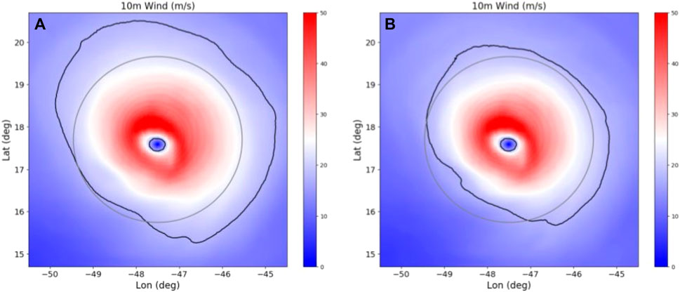
Figure 2. The total adjusted 10 m wind speed with two wind enhancement methods. (A) using a spatially constant
The modified VI package can then be directly used in the SHiELD workflow, which is based on the standard UFS_UTILS suite (https://ufs-community.github.io/UFS_UTILS/). Figure 3A illustrates the workflow of a typical forecast based on SHiELD that cold starts from IC files. We first create IC files for a specific date and time by remapping the corresponding GFS analysis to the model horizontal grids. And then the forecast job for this initial time can be launched directly using the IC files and other required external datasets.
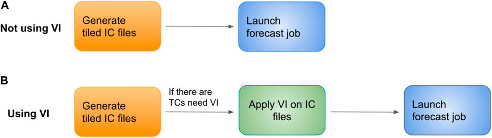
Figure 3. The workflow for launching a SHiELD forecast. (A) not using Vortex Initialization (VI) and (B) using VI.
In our proposed workflow that incorporates VI (Figure 3B), VI is introduced as an additional step in the preprocessing procedure. After generating the IC files, we apply the VI procedure to them if there are TCs that satisfy the user-specified criteria (e.g., the observed storm intensity exceeds a threshold value). If multiple storms require VI, the VI procedures can be applied sequentially, one storm after another. Note that we do not adopt cycling, even with VI incorporated. The forecast job is still cold started, but launched with the VI-adjusted IC files.
To demonstrate the impact of using our modified VI method on TC prediction, we conducted experiments using the T-SHiELD configuration, which is a two-way nested configuration of SHiELD (Harris et al., 2020; Gao et al., 2021) that features a large high-resolution nest (3.25 km grid spacing) over the North Atlantic (Figure 4).

Figure 4. Grid layout of the two-way nested T-SHiELD. Each plotted cell represents 48 × 48 actual grid cells. Heavy black lines represent cubed-sphere edges; red lines represent nested grids. The horizontal resolution is about 13 km in the global tile and 3.25 km in the nest (a refinement ratio of 4 is applied).
The hindcast experiments spanned August and September from 2020 to 2022, with initialization at 00:00 UTC and 12:00 UTC. We only considered the cases in which there was at least one storm with an observed maximum surface wind speed greater than 20 m/s (which is our VI threshold) in the nested region of T-SHiELD. We conducted two sets of T-SHiELD experiments, one with and the other without VI. The VI procedures are only applied to the IC files for the nested region.
We begin by examining the prediction of track, intensity and gale-forece wind radii (R34) of two selected hurricanes to gain a direct understanding of the impact of VI on individual TC predictions. Here R34 refers to the mean value of the gale-force wind radii averaged over the four quadrants. All track, intensity and wind radii values from the model were diagnosed using the GFDL Vortex Tracker (Marchok 2021).
Figure 5 shows the prediction for Hurricane Larry (2021) initialized on 2021-09-05 00:00 UTC. Using VI only has minor impact on the predicted track, which is somewhat expected, given that we only made modifications on the initial TC vortex but not the environment or the steering flow. There are significant impacts on the predicted storm intensity and R34. Most notably, the gap between the model and observed intensity at initiation (∼10 m/s) is effectively closed (Figure 5B).
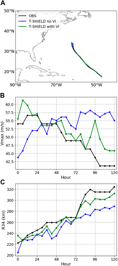
Figure 5. Prediction of Hurricane Larry initialized on 2021-09-05 00:00 UTC. (A) track, (B) intensity as measured by maximum 10 m wind speed, and (C) the mean gale-force wind radii (four-quadrant mean value is shown).
We further note that there is a benefit at longer lead time due to the improved initialization: the prediction for both intensity and R34 are improved even beyond day 3. This is an interesting finding considering that the model physics is not changed at all. The improvement at longer lead time here indicates that, at least for certain storms, the initialization of the storm intensity and structure has a long-lasting impact on storm evolution.
Figure 6 illustrates another successful case of using VI in the model, which is the prediction of Hurricane Fiona (2022), initialized on 2022-09-20 00:00 UTC. Similar to the Hurricane Larry (2021) case, there is little impact of using VI on track prediction, but VI effectively reduced the initial storm intensity bias. We also noted that the model predicted intensity and R34 of Fiona were not significantly different from those in the forecast with the use of VI method beyond 24 h. This implies that the impact of VI may be storm dependent. This motivates us to further examine the mean impact of using VI on multi-season statistics, which will be addressed in the following section.
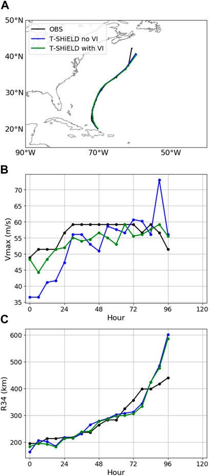
Figure 6. Prediction of Hurricane Fiona initialized on 2022-09-20 00:00 UTC. (A) track, (B) intensity as measured by maximum 10 m wind speed, and (C) the mean gale-force wind radii (four-quadrant mean value is shown).
We next present the TC track, intensity and R34 prediction error statistics in the T-SHiELD hindcasts done in the 2020-2022 North Atlantic Hurricane seasons (Figures 7–9). In the verification, we exclude storms that do not meet the VI thresholds; therefore, the difference between the two sets of experiments can clearly demonstrate the impact of VI. The key points are summarized below.
• The net impact of using VI on mean track error is small (Figure 7), consistent with what we observed in the individual forecasts (Figures 5A, 6A).
• There is a significant reduction in the mean intensity forecast bias and error (Figure 8), primarily within the first 48 h. Over a longer lead time, the mean bias and error in the set using VI are nearly the same as the reference set.
• For predictions of surface wind structure, T-SHiELD struggles with a persistent negative R34 forecast bias (Figure 9), suggesting that certain physical processes affecting R34 are not well captured by the model. However, the improvements in mean R34 forecast bias and error when using VI are encouraging: the reductions in the mean R34 forecast biases and errors persist throughout the entire 5-day period, indicating that the outer wind changes introduced by using VI can last for an extended period.
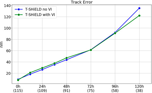
Figure 7. Mean track error from the two sets of T-SHiELD hindcast experiments with or without Vortex Initialization. The sample number for each lead time is shown in parenthesis.
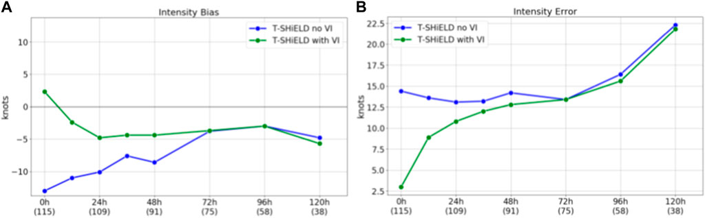
Figure 8. Same as Figure 7 but for (A) mean intensity bias and (B) mean intensity error.
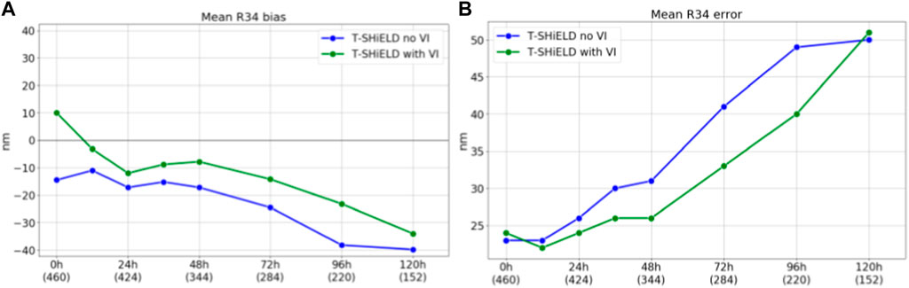
Figure 9. Same as Figure 7 but for (A) mean R34 bias and (B) mean R34 error. R34 represents the four-quadrant-mean gale-force wind radii. The number in the parentheses indicates the total number of data records used.
To summarize, we observe several benefits of using VI in the T-SHiELD experiments and there is no noticeable degradation in the model forecast skills. This led us to decide to incorporate VI in the workflow for the near real-time T-SHiELD for the 2023 hurricane season.
The VI package can easily be implemented in other SHiELD configurations to improve the TC representation in the IC. The benefits in 3.25 km resolution T-SHiELD motivate us to further assess the impact of VI in coarser-resolution SHiELD configurations. One SHiELD configuration under development at GFDL is the global uniform 6.5 km resolution SHiELD, which represents our most recent effort towards using global storm resolving-resolution for medium-range weather forecasting across the globe (a documentation paper is currently being prepared).
We next conducted exploratory experiments to probe the potential impact of using VI on TC forecasting at 6.5 km resolution. Considering the computational challenge involved in running the model at 6.5 km resolution globally, we introduce a reduced-resolution version of T-SHiELD, with a similar domain setup as T-SHiELD (Figure 4), but with the horizontal grid spacing in the nested region changed to 6.5 km. Similar to the two sets of T-SHiELD hindcasts we discussed in previous sessions, we conducted another two sets of hindcasts using the 6.5 km resolution nested configuration, one with VI and the other without.
The primary goal of using VI is to improve TC intensity and we therefore only focus on the storm intensity verification in these two sets of experiments (Figure 10). As expected, reducing the model resolution has a detrimental effect on TC intensity forecast skill across the entire 5-day period. However, we emphasize that the use of VI leads to significant improvement in the TC intensity forecast skill at 6.5 km resolution. Firstly, both the mean intensity bias and error in the first 24 h are significantly reduced, which is consistent with the finding from the 3.25 km resolution T-SHiELD experiments in Section 4.2. Secondly, the mean intensity error at even longer lead time is reduced because of the use of VI. The mean intensity errors on Days 4 and 5 in the 6.25 km resolution VI experiments are even close to those in the 3.25 km resolution T-SHiELD. These preliminary results suggest that correcting the initial TC intensity and structural biases with VI in the global uniform 6.5 km resolution SHiELD could have nontrivial impact on the TC intensity prediction. This finding underscores the need for additional efforts in this area. These results also imply that VI may be beneficial in lower-resolution prediction models and not just in kilometer-scale T-SHiELD and HAFS.
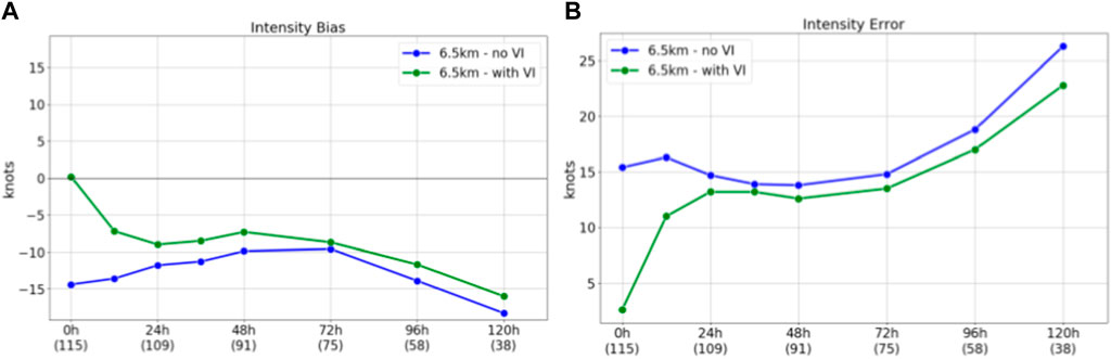
Figure 10. (A) Mean intensity bias and (B) intensity error from experiments done with a 6.5 km horizontal resolution nested SHiELD configuration (see text in Section 4.3 for details).
The main goal of this paper is to document the development and implementation of a Vortex Initialization (VI) technique in the GFDL SHiELD applications. We started with the publicly-released VI package implemented in the operational Hurricane Analysis and Forecast Model and made several modifications to facilitate its implementation in the SHiELD workflow, which includes the modifications made to the handling initial condition data, reducing input domain size, and improving storm intensity enhancement. Our proposed VI workflow can be easily implemented in any SHiELD application.
We conducted experiments using the T-SHiELD configuration, a global nested model with a 3.25 km-resolution two-way nest over the North Atlantic. Results show that incorporating VI effectively improves the representation of the initial TC intensity and size, and also improves TC prediction, particularly in storm intensity and outer wind predictions within the first 48 h. The impact on storm outer wind is observed even at longer lead times, indicating the lasting effects of improved initialization. Moreover, exploratory experiments conducted using a 6.5 km resolution configuration suggest that similar benefits may be seen even at coarser-resolution SHiELD configurations.
The results presented in this work are only our initial efforts. In our current VI implementation, we still cold start the model from GFS analysis and the wind increments for storm intensity enhancement are taken from a predefined synthetic vortex. The wind increments are vertically uniform and did not have a typical boundary layer flow structure. This could cause a sudden weakening of the TC intensity in the first 6 h or so as. Future work will focus on improving the storm enhancement strategy by either improving the structure of the predefined synthetic vortex, or using the spun up TC vortex from the previous forecast.
The datasets presented in this study can be found in online repositories. The names of the repository/repositories and accession number(s) can be found in the article/supplementary material.
KG: Conceptualization, Formal Analysis, Methodology, Software, Visualization, Writing–original draft, Writing–review and editing. LH: Funding acquisition, Writing–review and editing. MT: Conceptualization, Writing–review and editing. LZ: Writing–review and editing. J-HC: Writing–review and editing. K-YC: Software, Writing–review and editing.
The author(s) declare financial support was received for the research, authorship, and/or publication of this article. This research was funded by award NA23OAR4320198 from the National Oceanic and Atmospheric Administration, U.S. Department of Commerce. This work was substantively supported by the NOAA Research Global-Nest Initiative.
The authors would like to thank Tim Marchok and Jie Chen for discussions during the preparation of this manuscript, and the two reviewers for providing insightful comments.
The authors declare that the research was conducted in the absence of any commercial or financial relationships that could be construed as a potential conflict of interest.
All claims expressed in this article are solely those of the authors and do not necessarily represent those of their affiliated organizations, or those of the publisher, the editors and the reviewers. Any product that may be evaluated in this article, or claim that may be made by its manufacturer, is not guaranteed or endorsed by the publisher.
The statements, findings, conclusions, and recommendations are those of the authors and do not necessarily reflect the views of the National Oceanic and Atmospheric Administration, or the U.S. Department of Commerce.
Gao, K., Harris, L., Zhou, L., Bender, M. A., and Morin, M. J. (2021). On the sensitivity of hurricane intensity and structure to horizontal tracer advection schemes in FV3. J. Atmos. Sci. 78, 3007–3021. doi:10.1175/jas-d-20-0331.1
Harris, L., Zhou, L., Lin, S., Chen, J., Chen, X., Gao, K., et al. (2020). GFDL SHiELD: a unified system for weather-to-seasonal prediction. J. Adv. Model. Earth Syst. 12. e2020MS002 223. doi:10.1029/2020ms002223
Kurihara, Y., Bender, M., Tuleya, R., and Ross, R. (1995). Improvements in the GFDL hurricane prediction system. Mon. Weather Rev. 123, 2791–2801. doi:10.1175/1520-0493(1995)123<2791:iitghp>2.0.co;2
Kurihara, Y. M., Bender, M. A., and Ross, R. J. (1993). An initialization scheme of hurricane models by vortex specification. Mon. Wea. Rev. 121, 2030–2045. doi:10.1175/1520-0493(1993)121<2030:aisohm>2.0.co;2
Landsea, C. W., and Franklin, J. L. (2013). Atlantic hurricane database uncertainty and presentation of a new database format. Mon. Wea. Rev. 141 (10), 3576–3592. doi:10.1175/mwr-d-12-00254.1
Liu, Q., Zhang, X., Tong, M., Zhang, Z., Liu, B., Wang, W., et al. (2020). Vortex initialization in the NCEP operational hurricane models. Atmosphere 11, 968. doi:10.3390/atmos11090968
Tong, M., Sippel, J. A., Tallapragada, V., Liu, E., Kieu, C., Kwon, I. H., et al. (2018). Impact of assimilating aircraft reconnaissance observations on tropical cyclone initialization and prediction using operational HWRF and GSI ensemble–variational hybrid data assimilation. Mon. Weather Rev. 146, 4155–4177. doi:10.1175/mwr-d-17-0380.1
Keywords: hurricanes, tropical cyclones, high-resolution modeling, intensity forecast, initialization
Citation: Gao K, Harris L, Tong M, Zhou L, Chen J-H and Cheng K-Y (2024) A flexible tropical cyclone vortex initialization technique for GFDL SHiELD. Front. Earth Sci. 12:1396390. doi: 10.3389/feart.2024.1396390
Received: 05 March 2024; Accepted: 11 April 2024;
Published: 16 May 2024.
Edited by:
Zhan Zhang, NCEP Environmental Modeling Center (EMC), United StatesReviewed by:
Yuqing Wang, University of Hawaii at Manoa, United StatesCopyright © 2024 Gao, Harris, Tong, Zhou, Chen and Cheng. This is an open-access article distributed under the terms of the Creative Commons Attribution License (CC BY). The use, distribution or reproduction in other forums is permitted, provided the original author(s) and the copyright owner(s) are credited and that the original publication in this journal is cited, in accordance with accepted academic practice. No use, distribution or reproduction is permitted which does not comply with these terms.
*Correspondence: Kun Gao, a3VuLmdhb0Bub2FhLmdvdg==
Disclaimer: All claims expressed in this article are solely those of the authors and do not necessarily represent those of their affiliated organizations, or those of the publisher, the editors and the reviewers. Any product that may be evaluated in this article or claim that may be made by its manufacturer is not guaranteed or endorsed by the publisher.
Research integrity at Frontiers
Learn more about the work of our research integrity team to safeguard the quality of each article we publish.