Intermediate complexity atmospheric modeling in complex terrain: is it right?

Dynamic downscaling of atmospheric forcing data to the hectometer resolution has shown increases in accuracy for landsurface models, but at great computational cost. Here we present a validation of a novel intermediate complexity atmospheric model, HICAR, developed for hectometer scale applications. HICAR can run more than 500x faster than conventional atmospheric models, while containing many of the same physics parameterizations. Station measurements of air temperature, wind speed, and radiation, in combination with data from a scanning Doppler wind LiDAR, are compared to 50 m resolution HICAR output during late spring. We examine the model’s performance over bare ground and melting snow. The model shows a smaller root mean squared error in 2 m air temperature than the driving model, and approximates the 3D flow features present around ridges and along slopes. Timing and magnitude of changes in shortwave and longwave radiation also show agreement with measurements. Nocturnal cooling during clear nights is overestimated at the snow covered site. Additionally, the thermal wind parameterization employed by the model typically produces excessively strong surface winds, driven in part by this excessive nocturnal cooling over snow. These findings highlight the utility of HICAR as a tool for dynamically downscaling forcing datasets, and expose the need for improvements to the snow model used in HICAR.

1 Introduction

The state of the atmosphere is intertwined with land surface processes in a myriad of ways, affecting surface mass and energy balances through wind driven transport or radiative forcing, to name just two. The scales of these processes are often very heterogeneous, with ridges and depressions modifying the wind field over horizontal scales of tens of meters (Raderschall et al., 2008; Mott et al., 2010; Sauter and Galos, 2016). While land surface models have been run at the spatial scales of these heterogeneous processes for decades (Lehning et al., 2006; Liston and Elder, 2006; Sauter et al., 2020), they are not responsible for simulating these processes themselves. Instead, information about these processes are passed to land surface models through the atmospheric forcing data supplied to the models. One way of obtaining this forcing data is through dynamic downscaling, where atmospheric models are forced with coarse-resolution atmospheric data and run at a target horizontal resolution. Dynamic downscaling has been used at the scale of tens of kilometers for downscaling reanalysis data (Bozkurt et al., 2019) and has led to improvements in representing land surface processes at these scales (Gao et al., 2017; Sharma et al., 2023). Applications of dynamic downscaling for forcing land surface models at the hectometer scale are sparse, but similarly show improvements over other downscaling techniques (Vionnet et al., 2017; Voordendag et al., 2023). However, the computational demands of dynamic downscaling to the hectometer scale limit the application to short time series (hours to days) and small domains (catchment scale) (Sauter and Galos, 2016; Gerber et al., 2018; Vionnet et al., 2021; Goger et al., 2022; Saigger et al., 2023)).

This has led to widespread use of statistical downscaling in the land surface modeling community at the hectometer resolution. Statistical downscaling techniques have yielded reasonable simulations of seasonal snowpack (Winstral and Marks, 2002; Dadic et al., 2010), but often fail to capture inter-variable dependencies (Michel et al., 2021). Statistical downscaling treats variables in a “piece-wise” approach where each atmospheric variable is downscaled separately from one another. Thus dynamic downscaling is expected to better represent processes such as preferential deposition of snow (Lehning et al., 2008), where the interaction between terrain features and atmospheric stability induce changes in near-surface vertical winds, which in turn modify the deposition of precipitation (Wang and Huang, 2017). Additionally, statistical downscaling approaches may assume spatial patterns to be temporally fixed, limiting their use in climate change studies where the validity of these assumptions is unknown (Gutmann et al., 2012; Gutiérrez et al., 2013). Thus, although Physics-based dynamic downscaling has high computational costs, it remains attractive for many downscaling problems, especially under future climate scenarios.

To provide an alternative to weather models typically used in dynamic downscaling studies, the Intermediate Complexity Atmospheric Research (ICAR) model was proposed (Gutmann et al., 2016). ICAR was evaluated alongside the WRF model (Skamarock et al., 2008) in a previous study, showing predictive accuracy of wind speed and temperature similar to the WRF model at a handful of stations (Kruyt et al., 2022). However, the ICAR model suffered from little diurnal variability at a valley site, as well as a lack of ridge-scale flow features when compared to observations or the WRF model. These issues largely stem from ICAR being developed with a focus on downscaling to target resolutions at the kilometer scale, and not at the hectometer scale, where the evaluation was performed. To improve on these shortcomings, the High-resolution Intermediate Complexity Atmospheric Research (HICAR) model was recently introduced, addressing shortcomings in ICAR’s dynamics at high resolutions while still more than 500x faster than the WRF model (Reynolds et al., 2023). A direct validation of the HICAR model is still needed to understand how useful it may be for applications of dynamic downscaling. This study presents such a validation, focusing on processes which are of particular relevance to seasonal snowpack modeling. At the hectometer scale, flow features such as leeside recirculation, turbulent eddies, and thermally driven slope flows all dominate the near-surface flow field. Leeside recirculation can result in preferential deposition during snowfalls (Lehning et al., 2008), turbulent eddies enhance surface energy exchange (Haugeneder et al., 2024), and thermal flows effectively distribute surface heating throughout the surface layer (Farina and Zardi, 2023). This surface heating is itself driven by radiative forcing, which depends upon both cloud cover as well as topographic shading. HICAR’s ability to represent these processes is crucial for solving the surface energy balance and, particularly in the case of snowpack models, the surface mass balance.

This paper continues with section 2, where an overview of an observational campaign which occurred during winter 2021/2022 is given. Section 2 also contains a description of model changes implemented to represent some of the high-resolution processes discussed above. Section 3 presents a comparison of HICAR simulations with observations, focusing on near-surface flow features observed by a Doppler wind LiDAR. Lastly, a conclusion and summary of the study’s main points are given in section 4.

2 Methods

2.1 Observational campaign

In late April and Early May of 2022, a field campaign was conducted over a mountainous region outside of Davos, Switzerland, in the eastern Swiss Alps (Figure 1). A wind LiDAR (Section 2.1.1) was deployed within this domain, and five existing automatic weather stations (AWS) nearby recorded air temperature, wind speed, and wind direction during the period of the campaign. One station, located at the exposed summit Weissfluhjoch (WFJ), lies roughly 2 km south of and 400 m above the wind LiDAR. In this way, the WFJ station gives an estimate of the mesoscale conditions over the study area. The five stations included in the study are a part of two different measurement networks: the Swiss Meteorological Network (SMN) and the Intercantonal Measurement and Information System (IMIS). Sensors in the SMN feature ventilated temperature sensors, while the sensors in the IMIS network feature standard, solar-shaded temperature sensors. For wind sensors, IMIS stations sport propeller-type anemometers, while the SMN stations have 2D sonic anemometers.

Figure 1

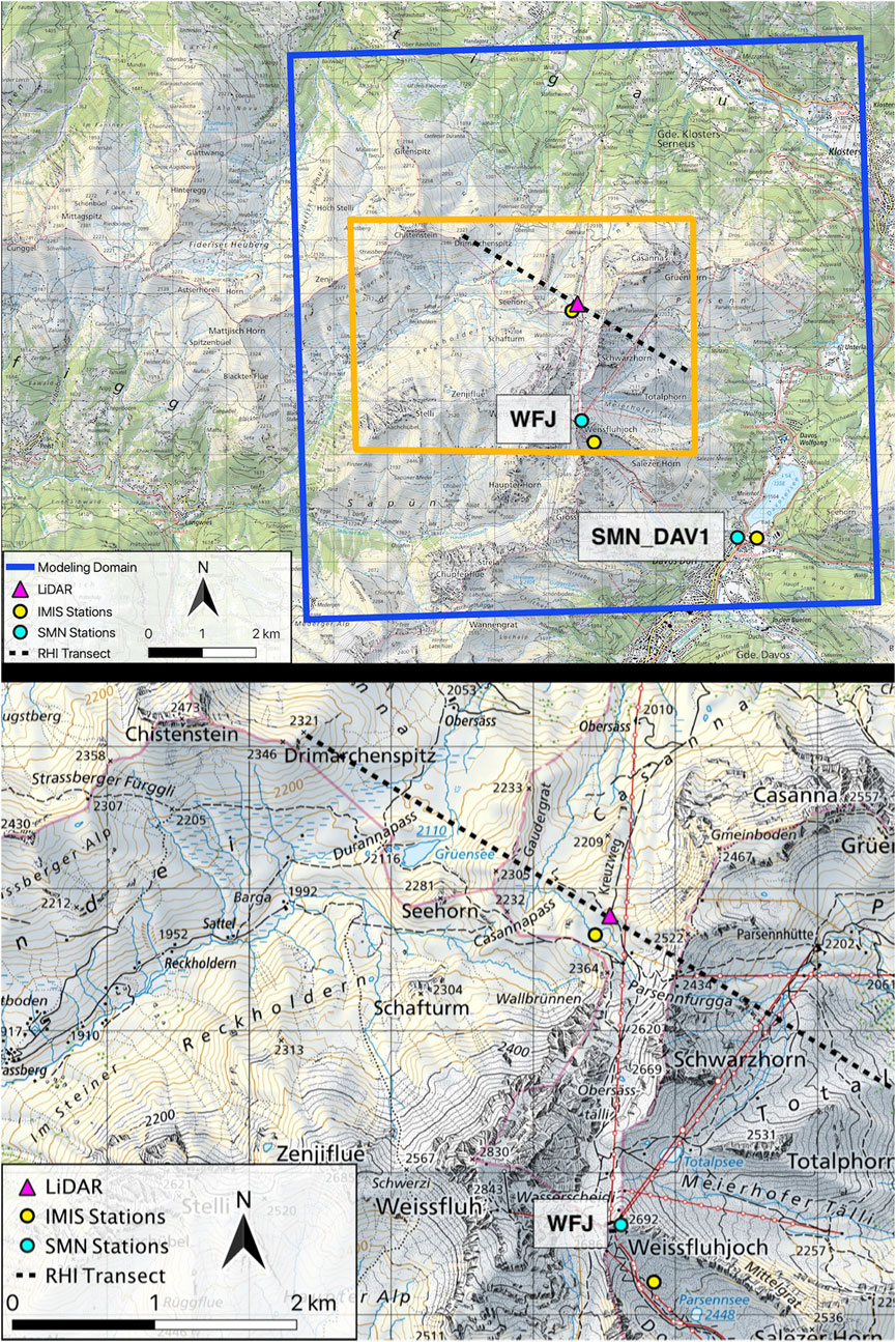
Figure 1. Map of the study domain. The upper panel shows the region around Weissfluhgipfel in the eastern Swiss Alps. The cyan dots indicate the location of the Swiss Meteorological Network (SMN) weather stations, which feature ventilated temperature sensors. The yellow dots correspond to stations from the Intercantonal Measurement and Information System (IMIS). The WFJ and SMN_DAV1 SMN stations shown in Figures 3, 4 are labeled. 50 m HICAR simulations were performed over the area contained within the blue square. The orange rectangle indicates the region shown in detail in the lower panel. This area focuses on the region around the wind LiDAR deployment, with the wind LiDAR shown as a pink triangle, and the orientation of the RHI scans presented in Section 3 given by the dashed black line. Of note are the Gaudergrat and Parsennfurgga, which the RHI transect crosses to the left and the right of the LiDAR, respectively.

2.1.1 Wind LiDAR scans

To validate the representation of wind speeds and flow features in HICAR, a Halo Photonics Streamline Doppler LiDAR was deployed. The ridge of Gaudergrat lies roughly the same elevation to the west of the location, while the pass Parsennfurgga rises over the LiDAR to the east. RHI (Range-Height Indicator) scans, where the laser is swept through a vertical slide of the atmosphere, were conducted every half hour. These scans sampled the flow structures over both aforementioned terrain features, starting over the Gaudergrat and ending at Parsennfurgga. The LiDAR was deployed from April 22nd to May 10th, with atmospheric conditions supporting good scan returns from May 1st to May 5th.

2.1.2 RHE scans

In addition to conventional RHI scans, we also introduce a new scan type, Reynolds-Haugeneder Elevation (RHE) scans. RHE scans are similar to PPI (Plan Position Indicator) scans, where azimuthal angle changes with a fixed elevation angle. However, for RHE scans, elevation angles are allowed to change for each azimuthal scan angle. Elevation angles are chosen such that the distance between the laser and underlying terrain maxima is minimized. In this way, the ridge crest flow is best sampled for all points around the LiDAR. RHE scans are created by taking a high-resolution DEM of the LiDAR area, and shooting rays outward from the position of the LiDAR at each of the azimuthal scan angles (Figure 2). These rays increase in elevation angle, from 0° upwards until they no longer intersect the surrounding DEM. This elevation angle is then saved as the elevation angle for the current azimuthal angle, and the next azimuthal angle is considered. RHE scans avoid large overshoots of the terrain which occur in PPI scans, and which are not helpful when validating near-surface flow features.

Figure 2

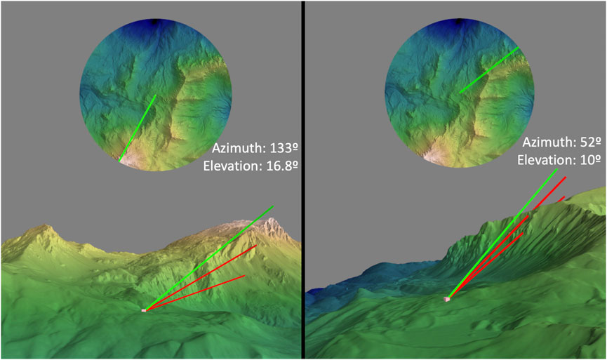
Figure 2. Schematic of how RHE scan angles are determined. The upper, circular graphics show the domain from above, with north facing upward. The green line cutting across the circle corresponds to the scan line from the wind LiDAR. In the bottom of the two panels, the view of the LiDAR in the terrain is shown, with the process of iteratively increasing the elevation angle until it clears the terrain. The azimuth of each scan, and the resultant scan elevation determined, is shown.

2.2 Model changes

The measurements in section 2.1 were conducted to validate a novel atmospheric model, HICAR (Reynolds et al., 2023). This model lacks a traditional Navier-Stokes-based dynamical core, and instead treats the 3D wind components as diagnostic variables when computing a mass-conserving wind field (Sherman, 1978; Forthofer et al., 2014). This saves significant computational time, but the predicted flow structures have not yet been validated against observations. In addition to the near-surface flow parameterizations existing in HICAR, a parameterization of thermal flows has also been introduced since the publication of (Reynolds et al., 2023). The following sections detail model changes relevant to this thermal-flows parameterization. The terrain parameters required in the following sections, including those for terrain-shading of radiation and the ridge distances for the slope flow parameterization, can be calculated using a python script contained in the HICAR distribution.

2.2.1 Thermal flow parameterization

One potential application of HICAR is modeling the seasonal snowpack. In snow-covered environments, katabatic winds, and the interplay between katabatic and valley winds in the spring play an important role in the surface wind field (Haugeneder et al., 2024). To address this, a thermal flow parameterization has been added to HICAR following the formulation in Grisogono et al. (2015) based on the popular Prandtl model of thermal winds (Prandtl, 1942). This model extends an existing parameterization of thermal winds, that of Oerlemans and Grisogono (2002), which was tested over an alpine glacier and showed reasonable agreement with station observations up to a height of 13 m. The updated formulation in Grisogono et al. (2015) allows for a vertically varying thermal eddy diffusivity and for the inclusion of additional terms representing enhanced mixing due to induced near-surface temperature gradients during anabatic winds. A full derivation of their method is included in the above publication. One mechanism of note is that the strength of the thermal flow correction is largely dependent on the temperature anomaly between the surface and the air aloft, in this case 200 m above the surface. Another important feature of this enhanced parameterization is that it produces stronger thermal flows over shallower slopes than steeper ones. The physical reason for this is the adiabatic heating that occurs to an air mass as it descends to lower altitudes. This heating rate is balanced by cooling due to negative sensible heat fluxes. As a slope becomes steeper, an air mass descends more elevation, and thus experiences greater adiabatic heating, while covering less distance along the terrain where cooling of the air parcel may occur. For slopes of lower angle, the air parcel traverses a greater distance along the terrain to cover the same vertical drop, resulting in a greater net cooling of the air mass, a larger density difference to the surrounding air, and thus stronger katabatic winds. Modeling studies using LES simulations and observational campaigns have noted that slopes of intermediate angle should experience stronger katabatic flows when compared to steep slopes or very flat slopes (Zhong and Whiteman, 2008; Zardi and Whiteman, 2013). An LES study of upslope flows over slopes of various angles showed a similar dependency of maximum wind speed on slope angle, perhaps due to the same mechanism acting in reverse (Schumanndlr, 1990).

The thermal wind parameterization introduces a dependency of the winds on physics processes which are updated more frequently than model input data is ingested. In version 1.1 of HICAR, a new wind field was only solved for each input time step. To more tightly couple the model dynamics with the physics, an update to HICAR’s wind solver has been added, allowing for more frequent solutions to the wind field. In the current study, this has been set so that a new wind field is solved for every 10 minutes of simulation time, allowing for the modeled surface winds to respond to rapidly changing surface energy fluxes around sunrise and sunset.

2.2.2 Physics parameterizations

The new thermal flow parameterization in HICAR depends in part upon the surface sensible heat flux calculated by a land surface model. Daytime sensible heat fluxes are driven primarily by incoming radiation at the grid cell. To this point, the RRTMG radiation transfer scheme (Thompson et al., 2016) is used in HICAR to compute both direct and diffuse shortwave radiation, as well as incident longwave radiation (Thompson et al., 2016). These radiation fields are then modified to account for sloping terrain surfaces and occluded sky view from surrounding terrain (Mott et al., 2023). The computation of these terrain parameters, namely, horizon line and sky view fraction, is normally computationally expensive, especially for high-resolution domains with many grid points. We use the HORAYZON python library developed by Steger et al. (2022) to efficiently calculate these terrain parameters for our domain.

These terrain-modified radiation inputs are then passed to the land surface model (LSM). NoahMP has been added to both the ICAR and HICAR models, widening the choice of land surface process representations. NoahMP has also been modified in HICAR to allow for the incident direct and diffuse shortwave radiation amounts calculated by RRTMG to be used directly, instead of a fixed partitioning of 70% direct and 30% diffuse hard-coded into NoahMP. These modifications allow for NoahMP to give improved estimates of sensible heat flux in complex terrain. NoahMP contains its own formulation for calculating surface exchange coefficients, and is not coupled to the surface exchange coefficients calculated by the surface layer scheme. To improve the representation of surface-atmosphere energy exchange, in particular during stable conditions, we add the revised MM5 surface layer (Jiménez et al., 2012) scheme’s calculation of exchange coefficients to NoahMP. To make this change to NoahMP consistent with the rest of the model physics, the revised MM5 surface layer scheme itself has been added to the model, and coupled to the Yonsei University (YSU) PBL scheme (Hong et al., 2006).

Lastly, the ISHMAEL microphysics scheme (Jensen et al., 2017) has also been added to HICAR, with the necessary steps to couple it to the RRTMG radiation scheme. This novel microphysics scheme is part of the growing class of adaptive habit (AHAB) microphysics schemes capable of evolving solid hydrometeor shape through time. This ability is crucial for resolving particle fall speeds and, thus, mass and energy exchange rates between hydrometeors and the atmosphere. For these reasons, the ISHMAEL scheme is also expected to offer an improvement in cold-cloud microphysics relative to the Morrison microphysics scheme (Morrison et al., 2005) already included in HICAR (Woods et al., 2007). Taken together, the ISHMAEL scheme may improve patterns of snowfall deposition in complex terrain and the mass-energy exchange between hydrometeors and the atmosphere. To evaluate the impact of this novel microphysics scheme, we perform HICAR simulations with both the Morrison and ISHMAEL schemes in Section 3.

2.3 Modeling setup

To evaluate the HICAR model, it was run over a period covering the observational campaign described above. Following the methodology of Reynolds et al. (2023) and Gerber et al. (2018), elevation data from ASTER Global Digital Elevation Model V002 and Corine land use data were used (European Environment Agency, 2006; ASTGTM, 2019), with atmospheric forcing data coming from the COSMO1E model (www.cosmo-model.org). One caveat to the setup of this study which differs from the setup used in Reynolds et al. (2023) is the lack of vertical velocity data from COSMO1 during our simulation period. To generate the diagnostic wind field HICAR requires some initial estimate of the 3D wind field. It then computes a final wind field by eliminating divergence in the wind field while minimizing the difference between the initial and final wind fields. Without an input of vertical velocity from COSMO1, an initial vertical velocity field of 0 is passed to the diagnostic wind solver. The underlying assumption here is that one solution for the vertical velocity field which eliminates divergence would be the vertical velocity field used by COSMO1. If there is no bias in the initial guess (using a wind field of 0) then the solution which minimizes changes to the initial 3 d wind field should favor a solution close to the original COSMO1 vertical velocity.

Starting with forcing data from the 1.1 km horizontal resolution COSMO1E model, nested HICAR simulations were performed at horizontal resolutions of 1km, 250, 100, and 50 m. The blue square shows the final domain used for the 50 m simulations in Figure 1. Static data and forcing variables used from COSMO1E follow the methodology outlined in Reynolds et al. (2023). 1km simulation HICAR runs were run from 1 October 2021 to 10 May 2022, in order to spin up the seasonal snowpack present during the observational campaign. The higher resolution simulations performed for the period of the campaign were then initialized with the snow cover of their parent domain. The high-resolution 50 m simulations were run from April 25th to May 10th. HICAR uses the NoahMP land surface scheme to parameterize land-surface processes (Niu et al., 2011), the YSU PBL scheme, and the RRTMG radiation scheme. Starting at the 250 m resolution simulation, the parameterization of terrain-induced sheltering introduced in Reynolds et al. (2023) is used. This scheme uses a 3D version of the Sx parameter (Winstral and Marks, 2002) to reduce wind speeds in the lee of prominent terrain features. The effects of this parameterization on the near-surface flow field are investigated in Section 3.3. Lastly, the PBL scheme is turned on for all simulations, even down to a horizontal resolution of 50 m. PBL schemes are commonly turned off for atmospheric modeling setups in the gray zone (Chow et al., 2019), or a scale-aware scheme is used (Shin and Hong, 2015). These steps are done because the atmospheric model is assumed to resolve some of the turbulent eddies at these scales, and so parameterized mixing in the form of a PBL scheme should not “double-count” this turbulence. Because HICAR does not consider momentum in its solution of a wind field, it is not known how much turbulent motion the model does resolve. As will be discussed in Section 3.4, HICAR does not appear to resolve turbulent motion driven by vertical wind shear and buoyancy. For this reason, the YSU PBL scheme remains active for model runs at all resolutions.

To test the impact of different model settings on simulations of air temperature and winds, three different model setups were performed (Table 1): one run using the Morrison microphysics scheme and the thermal wind parameterization, HICAR_Mor_Therm, a run using the ISHMAEL microphysics scheme and the thermal wind parameterization, HICAR_ISH_Therm, and lastly a run with the ISHMAEL microphysics scheme and no thermal wind parameterization, HICAR_ISH. These different modeling strategies are only compared in Table 2 and Figure 10. At all other points in the paper, the HICAR_ISH_Therm run is used and referred to simply as “HICAR”.

Table 1

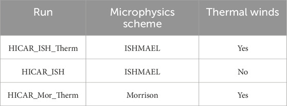
Table 1. Differences between model setups tested.

Table 2

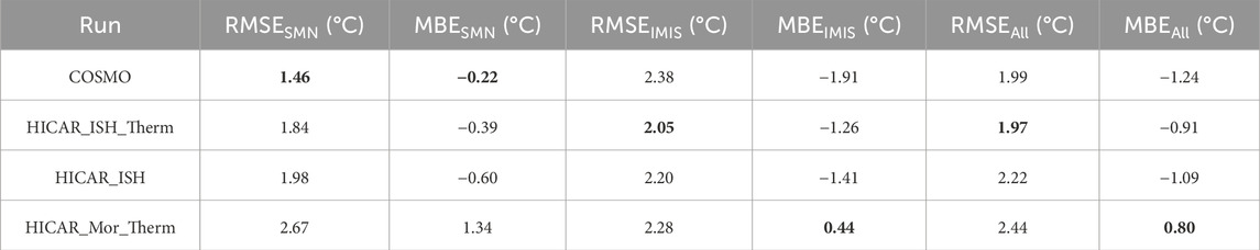
Table 2. Statistics of the 2 m air temperature estimates of various model runs as compared to observations. The X_SMN columns are values computed against the SMN stations, where ventilated temperature sensors are used. The IMIS stations are included as well in the X_IMIS and X_All columns to allow for more points of comparison. For the IMIS stations, times where wind speeds are less than 1.5 m/s are not considered in the analysis under the assumption that moderate wind speeds are enough to passively ventilate the sensors. The best score in each category is bolded.

3 Model evaluation

3.1 Point comparisons

Comparisons of 2 m air temperature, wind speed, and wind direction as measured at the AWSs SMN_DAV1 and WFJ and as modeled by HICAR are shown in Figure 3 from April 28th to May 10th. As seen in Figure 1, SMN_DAV1 is located on the valley bottom, while WFJ is located roughly 1,000 m above near a mountain peak. The three IMIS stations do not have ventilated temperature sensors, so only periods with wind speeds greater than 1.5 m/s are used in computing these statistics, assuming that this allows for some passive ventilation (Erell et al., 2005). These conditions of higher wind speeds tend to occur during the day, especially at the lower elevation stations that experience valley winds. Thus, when comparing against the IMIS stations, our comparison is biased toward mid day periods.

Figure 3

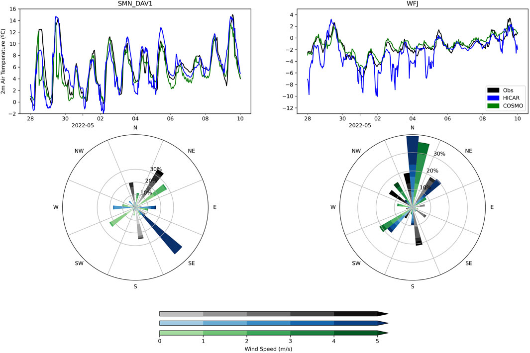
Figure 3. Comparisons of observations, the HICAR model, and the COSMO 1.1 km resolution model used to force the HICAR model. The upper plots show 2 m air temperature in °C from the two SMN stations. The lower plots show wind roses at the two sites calculated from observations of wind at 10 m height above ground. The data are grouped according to cardinal direction such that each data source can be compared with the others. The weight of the color indicates the wind speed, and the distance along the radial axis indicates the frequency of occurrence. As a reanalysis product, we stress that COSMO output data here has assimilated the SMN data in a post-processing step.

From the statistics of air temperature presented in Table 2 it is clear that the performance of HICAR depends on the microphysics scheme used. The Morrison microphysics scheme produces the highest positive mean bias error (MBE) of any of the model runs, with a MBE of 0.8°C across all AWSs in the modeling domain, and an MBE of 1.34°C at the ventilated SMN stations. At SMN stations, the ISHMAEL runs all show slight cold biases. These results suggest that the Morrison microphysics scheme results in slightly too warm of temperatures with our modeling setup. The cold biases of the ISHMAEL schemes may be attributable to the strong surface-atmosphere decoupling shown in Figure 3 which leads to very cold temperatures over snow on calm, clear nights. We thus expect that solving for these low biases would change the results such that the HICAR run with the Morrison microphysics scheme would no longer have the lowest MBE. The best results in RMSE are obtained once the thermal wind parameterization is switched on with the ISHMAEL microphysics scheme, yielding an RMSE of 1.97°C across all stations. This score is an improvement over the RMSE of the COSMO1 data (1.99°C), and the same run improves the MBE as well (−0.91°C for HICAR, −1.24°C for COSMO1), demonstrating HICAR’s added value as a downscaling scheme. For this reason, the rest of the analysis uses only the HICAR simulation with the ISHMAEL microphysics scheme and thermal winds.

Of note is the difference in performance when using all stations or simply the two SMN stations. As noted above, statistics including the IMIS stations are biased toward daytime measurements. At the high elevation station (WFJ) where a snow cover is present, HICAR displays excessive night time cooling during clear nights. Thus, biasing the period of observations towards daytime measurements benefits HICAR in this metric. Still, we include both sets of statistics, as using all stations increases the number of observations available for comparison. Additionally, the COSMO data has been assimilated to the SMN stations but not the IMIS stations, so this second group of AWSs is necessary.

When comparing the wind patterns at the valley site, the observations show strong winds coming from the up-valley direction (NE), and winds distributed roughly evenly along the up- and down-slope directions (N and S). The 1 km COSMO data simulates winds channeled along the valley axis (NE, SW), with overall lower wind speeds than the observations. HICAR shifts the distribution of the COSMO winds toward the up- and down-slope directions, unfortunately effectively removing any signal of channeled valley winds in the process. However, the wind speeds predicted by HICAR are higher than those of COSMO, and more inline with the observations. These findings suggest that the thermal wind parameterization, as implemented, results in excessive deflection of the input winds in the slope direction. At the WFJ site, winds are predominately affected by synoptic conditions, and thus little thermal flow signal is seen. Overall, the HICAR wind directions remain close to the wind directions predicted by COSMO. As observed at the valley site, however, wind speeds from HICAR are increased when compared to COSMO, better matching observations.

The differences in 2 m air temperature at the WFJ site are worth further discussion because of the dependency on radiative forcing that they highlight. In Figure 4 we observe that before sunset on April 30th, HICAR simulated cloudier conditions than observed. This is shown by the higher incoming longwave (LW) radiation and less outgoing shortwave (SW) radiation compared to observations. As a result, HICAR had higher temperatures than observations during this period (Figure 3). The opposite situation can be observed during the next night on May 2nd. HICAR simulates much colder temperatures than observed due to underestimating cloud cover. These results show a strong dependency of 2 m air temperature on the radiative forcing terms calculated by the RRTMG radiation scheme. It is possible that this strong dependency is compounded by underestimating turbulent fluxes during clear nights when stable conditions persist over the snow cover. This would result in excessive cooling of the near-surface layer. Previous studies using snow models have observed similar excessive nocturnal cooling of the snowpack, and suggest limiting the lower bound of the exchange coefficient under such stable conditions (Martin and Lejeune, 1998; Lafaysse et al., 2017; Mott et al., 2023). In a future study, we will explore the representation of snow-atmosphere interactions in more sophisticated snowpack models to improve this potential shortcoming.

Figure 4

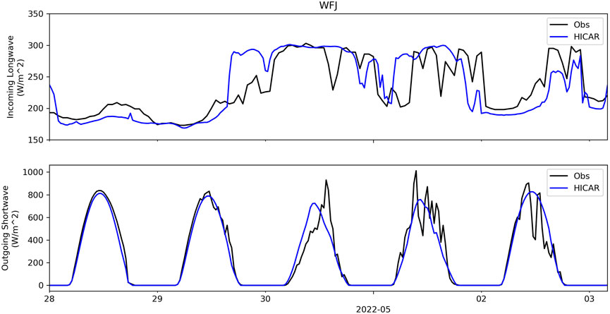
Figure 4. Observations of incoming longwave and outgoing shortwave at the WFJ SMN station compared to results from the HICAR model over a 5 day period. The choice of these variables was limited to the observations available at the WFJ station. The first 2 days have little cloud cover, as evident by the amount of incoming longwave, followed a period of intermittent cloudiness over the final 3 days. In the lower panel, the solid blue line indicates outgoing shortwave radiation as forecasted by HICAR, while the dashed blue line indicates outgoing shortwave radiation calculated using a constant surface albedo (α) of 0.8.

3.2 Ridge crest wind patterns

To investigate HICAR’s representation of spatial patterns of winds over exposed ridge crests, we employ the RHE scans introduced in Section 2.1.2. Figure 5 gives an example of an RHE scan. The bottom right panel shows the difference between scan elevation and terrain elevation. The upper right panel shows modeled wind vectors from HICAR overlaid on the terrain. Black arrows show the flow field in the first model level (∼10 m above ground), while gray arrows show the flow field in the second model level (∼30 m above terrain). It is already apparent that the thermal wind parameterization is highly localized to the first model level, and this point will be discussed later in Section 3.5. When comparing the terrain map in the upper right panel with the scan elevation difference in the bottom right, we see that the scan elevation is closest to the terrain over local terrain maxima. This approach maximizes our sampling of areas where terrain-induced speedup may be observed. The wind LiDAR scan shown in the bottom left panel indicates high radial velocities towards the LiDAR over Weissfluhgipfel in the bottom left corner of the panel. The general near-surface wind direction over the peak, as simulated by HICAR, runs mostly perpendicular to the axis of the RHI scans, indicated by the dashed black line. Radial velocities simulated by the HICAR model are shown in the upper left panel. These radial velocities are calculated from the 3D HICAR wind field by projecting the wind vector at each point along the scan vector from the wind LiDAR. The HICAR model simulates the high wind speeds over Weissfluhgipfel observed in the LiDAR data but overestimates the local reduction in wind speeds observed just south of the wind LiDAR location in the midslopes of Weissfluhgipfel. Using the modeled streamlines shown in the upper right panel, we can interpret this region of low radial velocities as being due to flow deflection around the ridge of Weissfluhgipfel. The scan elevation plot indicates that this region of the scan was slightly above the surface, so the synthetic RHE scan generated from the HICAR data is rather sampling the simulated flow field above the surface. The deflection simulated results in wind directions perpendicular to the LiDAR location, thus yielding near-0 radial velocities. Although the model overestimates this reduction, its ability to simulate the presence of such a fine-scale feature could still be considered a success of the model. Moving to the east of the Figure, wind speeds along the ridge crest containing Parsennfurgga can be examined. Here, we see good agreement between observed and modeled radial velocities, including predictions of radial velocity direction around the south-eastern axis of the RHI scan where the sign of radial velocity changes. Figure 10 shows a flow field as simulated by HICAR just a few days prior over Parsennfurgga. In the top panel, channelling of the synoptic scale winds through Parsennfurga, and the associated speed up, are resolved by the model. Over the summit of Schwarzhorn (the peak in the lower right of the figure), we do note that HICAR under predicts wind speeds, although the LiDAR data also suggest a local minimum in radial velocities over the peak compared to mid-slope wind speeds. Lastly, Figure 5 indicates that the synoptic-scale flow near the surface was oriented more westerly than HICAR predicts. This is evidenced by the line along which the sign of the radial velocity changes. Judging from the LiDAR data, it is observed to be slightly more horizontal than the line of sign reversal seen in the HICAR data, which roughly follows the axis of the RHI scan. This difference is likely due to the COSMO1 forcing data, which greatly confines the synoptic scale winds of the HICAR simulation. The dependency of the HICAR model on accurate forcing data results in an inability to correct for inaccurate input wind direction, although the difference between model and observations appears to only be on the order of $\approx 15°$. Taken together, we see that the HICAR model greatly relies on the input data used, but can add significant fine-scale detail to the simulated wind field, including regions of flow speed up, reduction, channeling, and deflection.

Figure 5

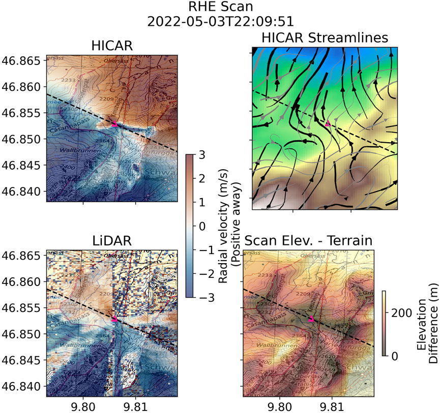
Figure 5. Demonstration of a Reynolds-Haugeneder Elevation (RHE) scan. The bottom right panel shows the difference in scan elevation relative to terrain elevation, with darker areas indicating scan locations closer to the surface. Radial velocities relative to the LiDAR location (pink triangle) are shown in the left panels, with the bottom panel showing data from the LiDAR scan and the upper panel output from the HICAR model. The dashed black line shows the orientation of the RHI scans discussed in later sections. The upper right panel shows modeled flow lines in the first model level in black, and flow lines in the second model level in gray.

3.3 Leeside structures

As outlined in Reynolds et al. (2023), HICAR features a parameterization for lee-side separation when the bulk Richardson number near the surface is below a critical threshold. The positioning of the wind LiDAR was chosen to scan into the leeside of a mountain ridge to validate this flow parameterization. Figure 6 shows the results of an RHI scan from the wind LiDAR for a time in the early morning of May 2nd. The scan shows flow moving from the east to the west over the Parsennfurgga. In these RHI figures, the perspective is that of a viewer standing north of the LiDAR and looking toward the south in Figure 1. As the flow encounters the ridge crest on the left, it seems to separate the lower-level airflow from the upper-level flow, creating an eddy-like structure on the lee side where we observe a reversal in the flow direction. This disturbance propagates downwind, with the flow reversal extending farther downwind than the location of the wind LiDAR. Weak wind speeds not exceeding $\approx 1$m/s are observed in this flow separation region. The results from HICAR accurately predict the occurrence of this eddy-like structure. The wind speeds within this region are also in approximate agreement with the observations from the LiDAR. The lateral extent of the eddy-like structure is different in the HICAR model as compared to observations. In HICAR, the parameterization for eddy extent relies on a user parameter for maximum extent and the bulk Richardson number in the lee side (Reynolds et al., 2023). Figure 6 indicates that the maximum extent of the lee side parameterization, which was set at 600 m in these simulations, may be limiting the growth of longer regions of flow recirculation. This highlights the promise of the existing parameterization for capturing non-local flow dynamics, but also the need for focused testing of the parameterization assumptions and functional relationships between terrain descriptors and flow modification.

Figure 6

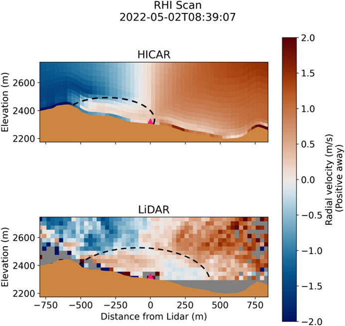
Figure 6. Radial velocities computed from the HICAR model relative to the position of the wind LiDAR (pink triangle), compared to observations of radial velocity from the LiDAR itself. Flow from the left to the right (east to west) over Parsennfurgga is seen to induce an area of recirculation behind the ridge. The approximate region of recirculation is marked with the dashed black line in both panels.

3.4 Turbulent flow features

An important distinction of the HICAR model is its lack of a mass and momentum-based solution to the wind field. This is one of the core advantages of the model in terms of computational speed, but also results in an expected under-performance for turbulent flows. Figure 7 illustrates such a scenario. The wind LiDAR observed easterly flow over the Gaudergrat around midday on May 4th, generating regions of alternating flow direction within the first 500 m above the surface. HICAR, however, simulates only one radial flow reversal as a function of height. This is likely produced by the leeside parameterization (Section 3.3), as both areas of flow reversal occur in the lees of Parsennfurga and Gaudergrat. Additionally, radial velocities of greater magnitude exist closer to the surface, due to either 1) the thermal flow parameterization, or 2) a rotation of the wind direction as a function of height. Since using a single wind LiDAR restricts us to comparisons of radial velocity, apparent flow reversal or increases in radial velocity in the RHI figures may be due to subtle rotations of the wind vectors towards or away from the LiDAR (best illustrated by consulting 5). Taken together, we can see that HICAR simulates unstable near-surface conditions, as evident by the activation of the leeside flow parameterization, and strong vertical shear near the surface. In reality, these combined factors should produce the turbulent near-surface flow observed by the wind LiDAR, but HICAR lacks any ability to consider vertical shear or buoyancy-driven turbulence in its flow modifications. This instance demonstrates HICAR’s inability to simulate turbulent flow under all atmospheric conditions.

Figure 7

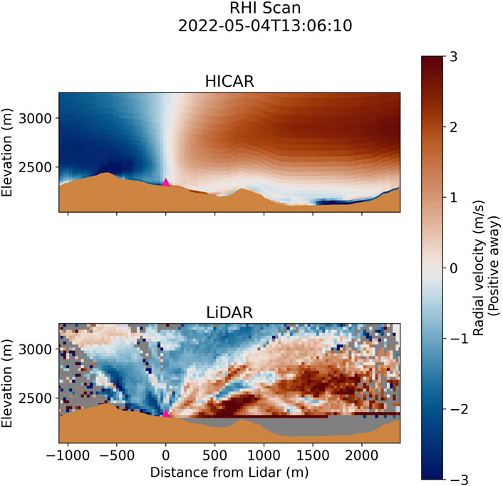
Figure 7. Radial velocities computed from the HICAR model relative to the position of the wind LiDAR (pink triangle), compared to observations of radial velocity from the LiDAR itself. Flow from the left to the right (east to west) over Gaudergratt creates turbulent structures which extend roughly 500 m aloft. The HICAR model simulates flow reversal relative to the wind LiDAR near the surface, but fails to capture any turbulent motions as observed.

3.5 Thermal flows

The model changes to HICAR, as detailed in Section 2.2.1, all seek to improve the model’s representation of the surface energy balance. Implementing a terrain-shading radiation parameterization and the direct coupling of RRTMG’s direct and diffuse shortwave radiation fields with the NoahMP land surface model are the main improvements contributing to this change in simulating surface energy fluxes. In the following discussion, positive sensible heat fluxes (Qs) corresponds to an upward heat flux, and negative Qs to a downward heat flux. The results of the model changes detailed earlier is indirectly on display in Figure 3, where the 2 m air temperature shows a clear diurnal signal and the effects of cloud cover. Figure 8 shows the heterogeneity in total modeled downwelling shortwave radiation throughout a day, centered on the deployed wind LiDAR (Figure 1). The differences in modeled shortwave radiation between the two daytime periods show the effects on radiative input induced by the complex terrain surrounding our site.

Figure 8

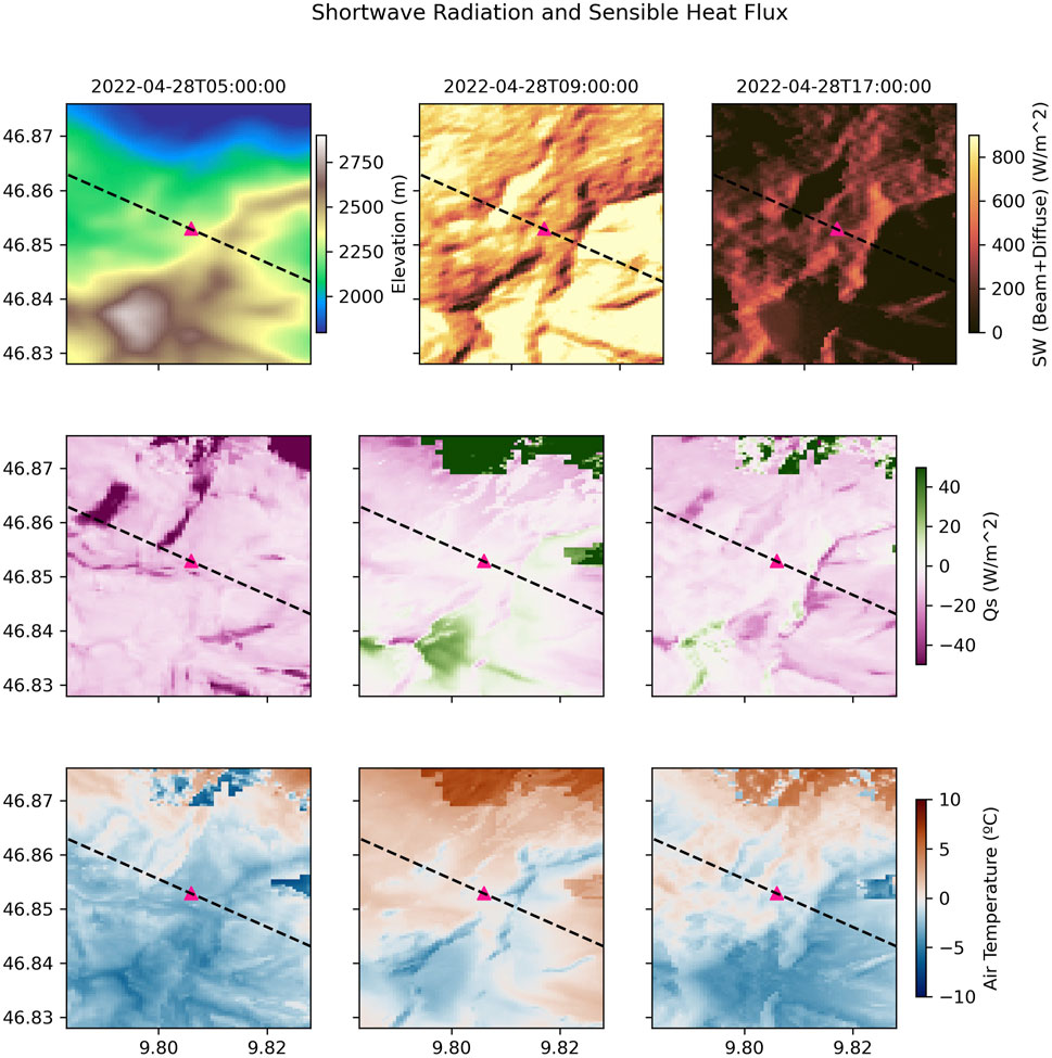
Figure 8. Downwelling shortwave radiation, sensible heat fluxes, and 2 m air temperature as modeled by HICAR from the pre-dawn hours on April 28th until 17:00 UTC. The upper left panel shows the orography over the region of interest. No plot of shortwave is shown for 5:00 UTC, as the sun was still below the horizon. The location of the wind LiDAR and orientation of the RHI transect are shown by the pink triangle and dashed black line, respectively.

This heterogeneity is also reflected in the maps of sensible heat flux. For the map at 9:00 UTC, high-elevation areas receiving more solar radiation generally experience a positive sensible heat flux as the snow cover over the domain heats up to 0°C. This is because the 2 m air temperature at these higher elevation areas is still below freezing at 9:00 UTC, resulting in a positive sensible heat flux. The sharp transition in sensible heat fluxes in the upper region of the figure is due to a transition from snow-covered, low-vegetation land surface types to forested model grid cells. NoahMP allows low-vegetation land surface types such as brush to become partly buried under snow, changing the surface albedo and exchange coefficients over such grid cells in comparison to forested grid cells. At 17:00 UTC, the pattern in sensible heat fluxes at high elevation areas is roughly reversed as the solar elevation angle swings across the sky, and the terrain shading parameterization captures the resultant effects on slope-scale shortwave irradiance. The high-elevation areas also experience more negative sensible heat fluxes at 17:00 UTC, as the overlaying air temperature is now above 0°C at the end of the clear, sunny day. For the map at the pre-dawn hour of 5:00 UTC, the pattern of sensible heat flux is seen to vary primarily with air temperature, with exposed areas tending to have sensible heat fluxes of greater magnitude due to stronger wind speeds driving greater surface energy exchange. These results for Figure 8 demonstrate the model’s ability to simulate heterogeneous patterns of surface energy fluxes.

Section 3.1 demonstrated the model’s ability to simulate downwelling radiative terms of the surface energy balance accurately. These terms are the driving forces behind the simulated 2 m air temperatures presented in Figure 3 and Table 2, which showed agreement with observations. We thus conclude that patterns of sensible heat fluxes shown in Figure 8 are reasonable, and now focus on the parameterization of thermally driven slope flows, which depend on these sensible heat fluxes.

The parameterization of slope flows follows the methodology outlined in Section 2.2.1. Figure 9 displays an RHI scan done in the early morning of May 3rd when little cloud cover was present and the snow-covered surface was able to cool due to longwave radiation. The LiDAR observations from this time show a thin layer of downslope flow moving toward the LiDAR from Parsennfurgga, and a reduction in wind speeds downwind from the LiDAR when compared to flow aloft. Lastly, flow away from the LiDAR is observed just over the crest of Gaudergrat. These observations suggest the presence of low-level slope flows down from Parsennfurgga, which entrain overlaying flow, slowing down the westerly flow aloft. Results from the HICAR model during this time show similar phenomena, with slope flows dominating the near-surface flow structure during this time. The primary difference between observations and HICAR is the difference in the vertical extent of the slope flows. Such strong vertical shear should induce turbulence, mixing up this near-surface layer. This would both lower the near-surface wind speeds, and distribute their influence vertically. HICAR’s approach to solving for the 3D wind field does not currently consider this process, and thus the strong vertical shear remains. One potential solution would be to modify the parameterization proposed by Grisogono et al. (2015) to smooth the correction to the wind field when shear is present. A broader picture is made available by Figure 10, illustrating the effect that this parameterization has on surface flows. The top panel shows wind speeds and direction at the 10 m height for a simulation run without the slope flow parameterization, while the bottom panel shows the same model output from a simulation run with the slope flow parameterization. The two primary effects of the parameterization appear to be both an increase in wind speeds along the downslope direction as well as a rotation of the mid-slope wind vectors to point more downslope. As a result, this effectively inhibits up-valley flow from spilling over the sub-ridge in the middle of Figure 10. During daytime hours over this late-season snow cover, air parcels from lower elevations tend to be heated due to their starting position over snow-free ground. The presence of balancing, katabatic flows produced by the snow cover is crucial to block the impingement of these warmer flows. Thus, the sort of lower-elevation flow-blocking displayed in Figure 10 is expected to be a necessary component of simulating late-season snow covers. As seen in Figure 3, the surface winds also reach higher speeds with the use of the thermal wind parameterization. The wind roses of the earlier figure suggest that the speed up shown in Figure 10 may be excessive.

Figure 9

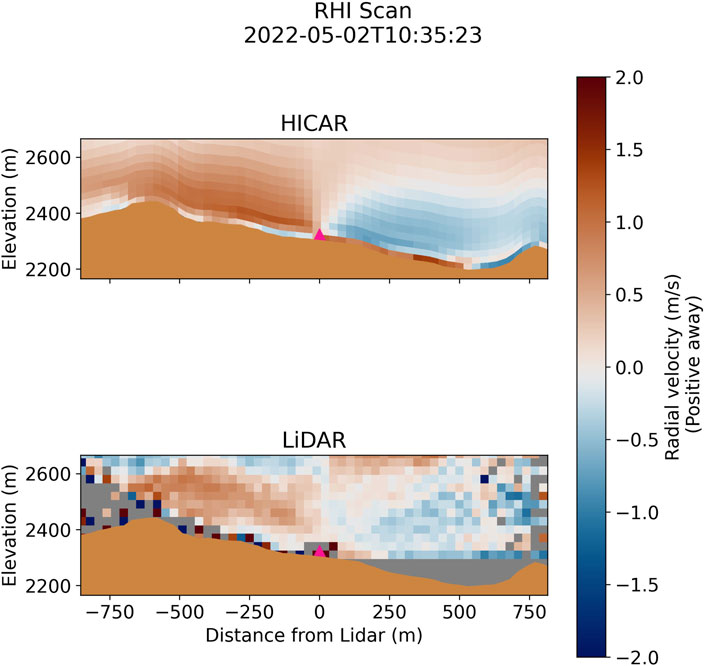
Figure 9. Radial velocities computed from the HICAR model relative to the position of the wind LiDAR (pink triangle), compared to observations of radial velocity from the LiDAR itself. Flow from the right to the left (west to east) is undercut by downslope flows running down from Parsennfurga and entraining air aloft.

Figure 10

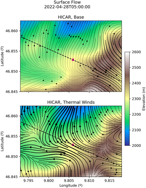
Figure 10. A comparison of modeled flow lines at 10 m height above ground for a 50 m resolution HICAR simulation without the thermal wind parameterization (top panel) and one with the parameterization (bottom panel). Thickness of the flow lines corresponds to wind speed, with thicker lines indicating higher wind speeds. For a time in the early morning hours over snow cover, the use of the thermal wind parameterization is shown to give stronger downslope flows.

4 Conclusion

This study assessed the efficacy of a new intermediate complexity atmospheric model designed for use at hectometer scales in alpine terrain. Three nested simulations were presented, stepping down to a simulation with a target resolution of 50 m run for 14 days. Each individual simulation takes an afternoon to run on a high-performance computing cluster, and consumes roughly 100 node-hours for the 210x213x40 simulation domain. As input, the model requires only topography and land cover data, as well as kilometer-scale output from a NWP model. With many regional weather forecasting offices now producing forecasts at this horizontal resolution, the study setup presented here could be repeated for numerous other locations. Ultimately this highly efficient setup allows for comparison of different physics options as done in this study. Such a comparison may be especially useful when used in combination with traditional, compressible atmospheric models.

Using sensors of incoming and outgoing radiation, air temperature, and wind speed, we have evaluated the model at valley bottom and mountain top sites in the late spring. During this time, ephemeral snowpack at high elevations significantly affects the exchange of energy between the surface and the atmosphere. The results overall demonstrate the clear added value of the HICAR model in its ability to improve forecasts of variables crucial to land-surface modeling. The findings of this study have particular relevancy to seasonal snowpack modeling, where forecasts of snowpack depend heavily on the surface energy balance, driven by downwelling radiation and air temperature, and accumulation processes influenced by winds and precipitation (Mott et al., 2023). Using measurements at several sites, we have found that using an adaptive-habit microphysics scheme improves the representation of 2 m air temperature while allowing for reasonable predictions of surface input radiation as affected by cloud cover. Additionally, the use of the thermal wind parameterization of Grisogono et al. (2015) improved simulated 2 m air temperature by allowing for improved near-surface ventilation during periods of surface radiative cooling. The mean bias error between one 50 m resolution HICAR simulation and five temperature sensors over a roughly 2-week period was found to be 0.18°C, compared to a mean bias error of −1.24°C for the driving model.

A spatial evaluation of the wind fields simulated by HICAR was conducted using data from a wind LiDAR deployed in complex, snow-covered terrain. A new type of LiDAR scan pattern, RHE scans, was also introduced and detailed, allowing maximum sampling of near-surface winds in complex terrain. The LiDAR device measured eddy-like structures in the leeside of terrain features and low-level thermally driven slope flows over the course of its 16-day deployment. Simulations with the HICAR model display similar features, demonstrating that the model can represent the presence and timing of such flow features. These interactions between terrain and flow are the primary drivers of flow field variability at these scales, and represent large modifications to the forcing wind field supplied by the 1.1 km COSMO data. Turbulent flow features were also observed by the wind LiDAR which HICAR can not represent. This is due to the lack of any consideration of momentum in the model’s solution of a 3D wind field.

Despite advantages for simulating 2 m air temperature when using the thermal wind parameterization, its use produced strong vertical gradients in wind speed. In reality, such strong vertical shear should produce mechanical mixing which allows for a transfer of momentum to higher altitudes. HICAR does not consider momentum, however, and so this shear remains in the wind field. Comparison of HICAR’s wind field at a valley station also showed that the thermal wind parameterization shifted the dominate flow regime from a mix of valley and slope flows to favoring almost exclusively slope flows. Both points indicate that the thermal flow correction is likely overestimated in the model, and requires some correction. An effect of vertical shear dampening could be approximated by modifying the thermal wind parameterization to apply a smoother correction.

Lastly, a large negative model bias in 2 m air temperature was observed over snow during clear nights. Due to the timing of this bias, and its presence in simulations both with and without the thermal wind parameterization we suspect that it is caused by overly inefficient exchange between the snow and atmosphere under stable conditions. As noted earlier, the snow modeling community has identified that current exchange parameterizations often produce excessively stable conditions over snow and result in excessive cooling of the snow surface (Martin and Lejeune, 1998; Schlögl et al., 2017). These shortcomings may be overcome by coupling HICAR to a more physically rigorous snowpack model, which will be explored in a future study. The period of evaluation chosen here, with heterogeneous snow cover and late-season storms of mixed precipitation phase, represents one of the most challenging periods of the snow season to correctly model. We thus anticipate the model performance to transfer well to periods of the snow season dominated either primarily solid precipitation or melt driven by incoming radiation. Coupling HICAR with land surface models may prove to be mutually beneficial, as these models would themselves benefit from high resolution atmospheric forcing data. Such a demonstration of a two-way coupled HICAR-snowpack model would prove the use of the model for applications where dynamic downscaling has long been attractive but remained technically prohibitive.

Data availability statement

HICAR can be used for non-profit purposes under the GPLv3 license (http://www.gnu.org/licenses/gpl-3.0.html, last access: 1 February 2023). Code for the model is available at https://github.com/HICAR-Model/HICAR. The exact release (v1.2) used in this publication is available at https://doi.org/10.5281/zenodo.10679307. Data from the IMIS stations are available at https://measurement-data.slf.ch/, data from the SMN stations are available at https://opendata.swiss/en/dataset/automatische-meteorologische-bodenmessstationen, and data from the Wind LiDAR observations are available at 10.16904/envidat.481. Output from the COSMO1 model was obtained through MeteoSwiss. The basemap layer used in Figure 1 comes from Swiss Topo. Similarly, topographic data for generating the RHE schematic and designing the scans was obtained from Swiss Topo swissALTI3d (https://www.swisstopo.admin.ch/de/hoehenmodell-swissalti3d).

Author contributions

DR: Conceptualization, Software, Writing–original draft, Writing–review and editing. MH: Conceptualization, Investigation, Writing–review and editing. ML: Conceptualization, Supervision, Writing–review and editing. RM: Conceptualization, Funding acquisition, Supervision, Writing–review and editing.

Funding

The author(s) declare financial support was received for the research, authorship, and/or publication of this article. The authors thank the funding source of this project, the Swiss National Science Foundation grant #188554.

Acknowledgments

The computational resources needed to perform the simulations were provided by the Swiss National Supercomputing Center (CSCS) through projects s1148 and sm78. The authors would like to thank Mahdi Jafari and Moritz Oberrauch for assisting in the retrieval of the wind LiDAR during challenging, late-season conditions. Fanny Kristianti and Franziska Gerber were also key in providing help and understanding of the Halo Photonics system. Developers of open source python toolboxes, particularly xarray and xesmf, have also played a crucial role in this study by enabling efficient analysis and manipulation of large datasets. The authors thank two reviewers for their contributions to the scientific process. The authors thank the funding.

Conflict of interest

The authors declare that the research was conducted in the absence of any commercial or financial relationships that could be construed as a potential conflict of interest.

The author(s) declared that they were an editorial board member of Frontiers, at the time of submission. This had no impact on the peer review process and the final decision.

Publisher’s note

All claims expressed in this article are solely those of the authors and do not necessarily represent those of their affiliated organizations, or those of the publisher, the editors and the reviewers. Any product that may be evaluated in this article, or claim that may be made by its manufacturer, is not guaranteed or endorsed by the publisher.

References

ASTGTM (2019). Aster global digital elevation model v003, nasa eosdis land processes daac. Distributed by NASA EOSDIS Land Processes DAAC.

Google Scholar

Bozkurt, D., Rojas, M., Boisier, J. P., Rondanelli, R., Garreaud, R., and Gallardo, L. (2019). Dynamical downscaling over the complex terrain of southwest south America: present climate conditions and added value analysis. Clim. Dyn. 53, 6745–6767. doi:10.1007/s00382-019-04959-y

CrossRef Full Text | Google Scholar

Chow, F. K., Schär, C., Ban, N., Lundquist, K. A., Schlemmer, L., and Shi, X. (2019). Crossing multiple gray zones in the transition from mesoscale to microscale simulation over complex terrain. Atmosphere 10, 274. doi:10.3390/atmos10050274

CrossRef Full Text | Google Scholar

Dadic, R., Mott, R., Lehning, M., and Burlando, P. (2010). Parameterization for wind–induced preferential deposition of snow. Hydrol. Process. 24, 1994–2006. doi:10.1002/hyp.7776

CrossRef Full Text | Google Scholar

Erell, E., Leal, V., and Maldonado, E. (2005). Measurement of air temperature in the presence of a large radiant flux: an assessment of assively ventilated thermometer screens. Boundary-Layer Meteorol. 114, 205–231. doi:10.1007/s10546-004-8946-8

CrossRef Full Text | Google Scholar

European Environment Agency (2006). Corine land cover (clc) 2006 raster data, version 13. Available at: https://www.eea.europa.eu/data-and-maps/data/clc-2006-raster.

Google Scholar

Farina, S., and Zardi, D. (2023). Understanding thermally driven slope winds: recent advances and open questions. Boundary-Layer Meteorol. 189, 5–52. doi:10.1007/s10546-023-00821-1

CrossRef Full Text | Google Scholar

Forthofer, J., Butler, B., and Wagenbrenner, N. (2014). A comparison of three approaches for simulating fine-scale surface winds in support of wildland fire management. part i. model formulation and comparison against measurements. Int. J. Wildland Fire 23, 969–981. doi:10.1071/WF12089

CrossRef Full Text | Google Scholar

Gao, Y., Xiao, L., Chen, D., Chen, F., Xu, J., and Xu, Y. (2017). Quantification of the relative role of land-surface processes and large-scale forcing in dynamic downscaling over the Tibetan plateau. Clim. Dyn. 45, 1705–1721. doi:10.1007/s00382-016-3168-6

CrossRef Full Text | Google Scholar

Gerber, F., Besic, N., Sharma, V., Mott, R., Daniels, M., Gabella, M., et al. (2018). Spatial variability in snow precipitation and accumulation in cosmo–wrf simulations and radar estimations over complex terrain. Cryosphere 12, 3137–3160. doi:10.5194/tc-12-3137-2018

CrossRef Full Text | Google Scholar

Goger, B., Stiperski, I., Nicholson, L., and Sauter, T. (2022). Large-eddy simulations of the atmospheric boundary layer over an alpine glacier: impact of synoptic flow direction and governing processes. Q. J. R. Meteorological Soc. 148, 1319–1343. doi:10.1002/qj.4263

CrossRef Full Text | Google Scholar

Grisogono, B., Jurlina, T., Večenaj, v., and Güttler, I. (2015). Weakly nonlinear Prandtl model for simple slope flows. Q. J. R. Meteorological Soc. 141, 883–892. doi:10.1002/qj.2406

CrossRef Full Text | Google Scholar

Gutiérrez, J. M., San-Martín, D., Brands, S., Manzanas, R., and Herrera, S. (2013). Reassessing statistical downscaling techniques for their robust application under climate change conditions. J. Clim. 26, 171–188. doi:10.1175/JCLI-D-11-00687.1

CrossRef Full Text | Google Scholar

Gutmann, E., Barstad, I., Clark, M., Arnold, J., and Rasmussen, R. (2016). The intermediate complexity atmospheric research model (icar). J. Hydrometeorol. 17, 957–973. doi:10.1175/JHM-D-15-0155.1

CrossRef Full Text | Google Scholar

Gutmann, E. D., Rasmussen, R. M., Liu, C., Ikeda, K., Gochis, D. J., Clark, M. P., et al. (2012). A comparison of statistical and dynamical downscaling of winter precipitation over complex terrain. J. Clim. 25, 262–281. doi:10.1175/2011JCLI4109.1

CrossRef Full Text | Google Scholar

Haugeneder, M., Lehning, M., Stiperski, I., Reynolds, D., and Mott, R. (2024). Turbulence in the strongly heterogeneous near-surface boundary layer over patchy snow. Boundary-Layer Meteorol. 190. doi:10.1007/s10546-023-00856-4

CrossRef Full Text | Google Scholar

Hong, S.-Y., Noh, Y., and Dudhia, J. (2006). A new vertical diffusion package with an explicit treatment of entrainment processes. Mon. Weather Rev. 134, 2318–2341. doi:10.1175/MWR3199.1

CrossRef Full Text | Google Scholar

Jensen, A. A., Harrington, J. Y., Morrison, H., and Milbrandt, J. A. (2017). Predicting ice shape evolution in a bulk microphysics model. J. Atmos. Sci. 74, 2081–2104. doi:10.1175/JAS-D-16-0350.1

CrossRef Full Text | Google Scholar

Jiménez, P. A., Dudhia, J., González-Rouco, J. F., Navarro, J., Montávez, J. P., and García-Bustamante, E. (2012). A revised scheme for the wrf surface layer formulation. Mon. Weather Rev. 140, 898–918. doi:10.1175/MWR-D-11-00056.1

CrossRef Full Text | Google Scholar

Kruyt, B., Mott, R., Fiddes, J., Gerber, F., Sharma, V., and Reynolds, D. (2022). A downscaling intercomparison study: the representation of slope- and ridge-scale processes in models of different complexity. Front. Earth Sci. 10. doi:10.3389/feart.2022.789332

CrossRef Full Text | Google Scholar

Lafaysse, M., Cluzet, B., Dumont, M., Lejeune, Y., Vionnet, V., and Morin, S. (2017). A multiphysical ensemble system of numerical snow modelling. Cryosphere 11, 1173–1198. doi:10.5194/tc-11-1173-2017

CrossRef Full Text | Google Scholar

Lehning, M., Löwe, H., Ryser, M., and Raderschall, N. (2008). Inhomogeneous precipitation distribution and snow transport in steep terrain. Water Resour. Res. 44. doi:10.1029/2007WR006545

CrossRef Full Text | Google Scholar

Lehning, M., Völksch, I., Gustafsson, D., Nguyen, T. A., Stähli, M., and Zappa, M. (2006). Alpine3d: a detailed model of mountain surface processes and its application to snow hydrology. Hydrol. Process. 20, 2111–2128. doi:10.1002/hyp.6204

CrossRef Full Text | Google Scholar

Liston, G. E., and Elder, K. (2006). A distributed snow-evolution modeling system (snowmodel). J. Hydrometeorol. 7, 1259–1276. doi:10.1175/JHM548.1

CrossRef Full Text | Google Scholar

Martin, E., and Lejeune, Y. (1998). Turbulent fluxes above the snow surface. Ann. Glaciol. 26, 179–183. doi:10.3189/1998AoG26-1-179-183

CrossRef Full Text | Google Scholar

Michel, A., Sharma, V., Lehning, M., and Huwald, H. (2021). Climate change scenarios at hourly time-step over Switzerland from an enhanced temporal downscaling approach. Int. J. Climatol. 41, 3503–3522. doi:10.1002/joc.7032

CrossRef Full Text | Google Scholar

Morrison, H., Curry, J. A., and Khvorostyanov, V. I. (2005). A new double-moment microphysics parameterization for application in cloud and climate models. part i: description. J. Atmos. Sci. 62, 1665–1677. doi:10.1175/JAS3446.1

CrossRef Full Text | Google Scholar

Mott, R., Schirmer, M., Bavay, M., Grünewald, T., and Lehning, M. (2010). Understanding snow-transport processes shaping the mountain snow-cover. Cryosphere 4, 545–559. doi:10.5194/tc-4-545-2010

CrossRef Full Text | Google Scholar

Mott, R., Winstral, A., Cluzet, B., Helbig, N., Magnusson, J., Mazzotti, G., et al. (2023). Operational snow-hydrological modeling for Switzerland. Front. Earth Sci. 11. doi:10.3389/feart.2023.1228158

CrossRef Full Text | Google Scholar

Niu, G.-Y., Yang, Z.-L., Mitchell, K. E., Chen, F., Ek, M. B., Barlage, M., et al. (2011). The community noah land surface model with multiparameterization options (noah-mp): 1. model description and evaluation with local-scale measurements. J. Geophys. Res. Atmos. 116, D12109. doi:10.1029/2010JD015139

CrossRef Full Text | Google Scholar

Oerlemans, J., and Grisogono, B. (2002). Glacier winds and parameterisation of the related surface heat fluxes. Tellus A Dyn. Meteorology Oceanogr. 54, 440–452. doi:10.3402/tellusa.v54i5.12164

CrossRef Full Text | Google Scholar

Prandtl, L. (1942). Führer durch die Strömungslehre. Braunschweig, Germany: Vieweg und Sohn.

Google Scholar

Raderschall, N., Lehning, M., and Schär, C. (2008). Fine-scale modeling of the boundary layer wind field over steep topography. Water Resour. Res. 44. doi:10.1029/2007WR006544

CrossRef Full Text | Google Scholar

Reynolds, D., Gutmann, E., Kruyt, B., Haugeneder, M., Jonas, T., Gerber, F., et al. (2023). The high-resolution intermediate complexity atmospheric research (hicar v1.1) model enables fast dynamic downscaling to the hectometer scale. Geosci. Model Dev. 16, 5049–5068. doi:10.5194/gmd-16-5049-2023

CrossRef Full Text | Google Scholar

Saigger, M., Sauter, T., Schmid, C., Collier, E., Goger, B., Kaser, G., et al. (2023). Snowdrift scheme in the weather research and forecasting model. Available at: https://essopenarchive.org/users/666025/articles/667036-snowdrift-scheme-in-the-weather-research-and-forecasting-model.

Google Scholar

Sauter, T., Arndt, A., and Schneider, C. (2020). Cosipy v1.3 – an open-source coupled snowpack and ice surface energy and mass balance model. Geosci. Model Dev. 13, 5645–5662. doi:10.5194/gmd-13-5645-2020

CrossRef Full Text | Google Scholar

Sauter, T., and Galos, S. P. (2016). Effects of local advection on the spatial sensible heat flux variation on a mountain glacier. Cryosphere 10, 2887–2905. doi:10.5194/tc-10-2887-2016

CrossRef Full Text | Google Scholar

Schlögl, S., Lehning, M., Nishimura, K., Huwald, H., Cullen, N. J., and Mott, R. (2017). How do stability corrections perform in the stable boundary layer over snow? Boundary-Layer Meteorol. 165, 161–180. doi:10.1007/s10546-017-0262-1

CrossRef Full Text | Google Scholar

Schumanndlr, U. (1990). Large-eddy simulation of the up-slope boundary layer. Q. J. R. Meteorological Soc. 116, 637–670. doi:10.1002/qj.49711649307

CrossRef Full Text | Google Scholar

Sharma, V., Gerber, F., and Lehning, M. (2023). Introducing cryowrf v1.0: multiscale atmospheric flow simulations with advanced snow cover modelling. Geosci. Model Dev. 16, 719–749. doi:10.5194/gmd-16-719-2023

CrossRef Full Text | Google Scholar

Sherman, C. A. (1978). A mass-consistent model for wind fields over complex terrain. J. Appl. Meteorology Climatol. 17, 312–319. doi:10.1175/1520-0450(1978)017<0312:amcmfw>2.0.co;2.CO;2

CrossRef Full Text | Google Scholar

Shin, H. H., and Hong, S.-Y. (2015). Representation of the subgrid-scale turbulent transport in convective boundary layers at gray-zone resolutions. Mon. Weather Rev. 143, 250–271. doi:10.1175/MWR-D-14-00116.1

CrossRef Full Text | Google Scholar

Skamarock, W. C., Klemp, J. B., Dudhia, J., Gill, D. O., Barker, D., and Duda, J. G. (2008). A description of the advanced research wrf version 3. University Corporation for Atmospheric Research.

Google Scholar

Steger, C. R., Steger, B., and Schär, C. (2022). Horayzon v1.2: an efficient and flexible ray-tracing algorithm to compute horizon and sky view factor. Geosci. Model Dev. 15, 6817–6840. doi:10.5194/gmd-15-6817-2022

CrossRef Full Text | Google Scholar

Thompson, G., Tewari, M., Ikeda, K., Tessendorf, S., Weeks, C., Otkin, J., et al. (2016). Explicitly-coupled cloud physics and radiation parameterizations and subsequent evaluation in wrf high-resolution convective forecasts. Atmos. Res. 168, 92–104. doi:10.1016/j.atmosres.2015.09.005

CrossRef Full Text | Google Scholar

Vionnet, V., Marsh, C. B., Menounos, B., Gascoin, S., Wayand, N. E., Shea, J., et al. (2021). Multi-scale snowdrift-permitting modelling of mountain snowpack. Cryosphere 15, 743–769. doi:10.5194/tc-15-743-2021

CrossRef Full Text | Google Scholar

Vionnet, V., Martin, E., Masson, V., Lac, C., Naaim Bouvet, F., and Guyomarc’h, G. (2017). High-resolution large eddy simulation of snow accumulation in alpine terrain. J. Geophys. Res. Atmos. 122. doi:10.1002/2017JD026947

CrossRef Full Text | Google Scholar

Voordendag, A., Goger, B., Prinz, R., Sauter, T., Mölg, T., Saigger, M., et al. (2023). Investigating wind-driven snow redistribution processes over an alpine glacier with high-resolution terrestrial laser scans and large-eddy simulations. EGUsphere 2023, 1–27. doi:10.5194/egusphere-2023-1395

CrossRef Full Text | Google Scholar

Wang, Z., and Huang, N. (2017). Numerical simulation of the falling snow deposition over complex terrain. J. Geophys. Res. Atmos. 122, 980–1000. doi:10.1002/2016JD025316

CrossRef Full Text | Google Scholar

Winstral, A., and Marks, D. (2002). Simulating wind fields and snow redistribution using terrain-based parameters to model snow accumulation and melt over a semi-arid mountain catchment. Hydrol. Process. 16, 3585–3603. doi:10.1002/hyp.1238

CrossRef Full Text | Google Scholar

Woods, C. P., Stoelinga, M. T., and Locatelli, J. D. (2007). The improve-1 storm of 1–2 february 2001. part iii: sensitivity of a mesoscale model simulation to the representation of snow particle types and testing of a bulk microphysical scheme with snow habit prediction. J. Atmos. Sci. 64, 3927–3948. doi:10.1175/2007JAS2239.1

CrossRef Full Text | Google Scholar

Zardi, D., and Whiteman, C. D. (2013). “Diurnal mountain wind systems,” in Mountain weather research and forecasting: recent progress and current challenges (Springer), 35–119.

CrossRef Full Text | Google Scholar

Zhong, S., and Whiteman, C. D. (2008). Downslope flows on a low-angle slope and their interactions with valley inversions. part ii: numerical modeling. J. Appl. Meteorology Climatol. 47, 2039–2057. doi:10.1175/2007JAMC1670.1

CrossRef Full Text | Google Scholar