 Ahmed S. Almohaimeed
- Department of Mathematics, College of Science, Qassim University, Buraydah, Saudi Arabia
In the atmosphere, the interrelationship between dynamics and chemistry results in mutual influence and interaction. The behavior of internal gravity waves is influenced by the thermal effects caused by chemical components present in the atmosphere. In this investigation, the equations determining gravity waves are coupled with those characterizing the behavior of ozone and water vapor. To investigate the coupled equations, numerical analyses are conducted, and the resulting numerical results are presented. Internal gravity waves have been observed to influence the distribution of ozone and water vapor within the Earth’s atmosphere. It has been demonstrated, based on our findings, that wave fluctuations play a significant role in exerting a substantial effect. In addition, it has been observed that the influence of ozone and water vapor-induced heating on gravity waves is significant, particularly near the critical level where the mean flow induced by gravity waves plays a significant role.
1 Introduction
The decline in atmospheric density as one moves away from the Earth’s surface results in the atmosphere being relatively stable and stratified. The combination of the buoyancy-restoring force resulting from stratification and the gravitational force gives rise to the formation of internal gravity waves.
Internal gravity waves often travel vertically in the atmosphere, either upwards or downwards, and have the potential to break down, resulting in a turbulent flow. The significance of gravity wave impacts escalates as altitude rises due to the exponential growth of gravity wave amplitude with altitude. Vertical mixing mostly occurs due to the breaking of gravity waves (Shepherd, 2007).
Internal gravity waves have a substantial role in influencing many meteorological and climatological events. The assessment of such influence has significant importance when simulating wind velocity and temperature within the natural surroundings. The phenomenon known as the “critical level” arises when the average velocity of fluid flow is equal to the speed at which a wave propagates. The critical level mentioned in this context is linked to a singularity seen in the linearized equations of gravity waves (GWs), as discussed by (Nappo, 2002; Marshall and Plumb, 2008). Clear-air turbulence is a phenomena defined by the turbulent movement of air, which may be linked to the occurrence of internal wave breaking. In the field of mathematical modeling, gravity waves are often shown using Fourier modes in spatial representation. The zero wavenumber mode component is linked to modifications in the average flow; such modifications lead to what is often known as the wave-induced mean flow (Sutherland, 2010).
The atmosphere consists of major chemical constituents such as nitrogen (N), oxygen (O), argon (Ar), water vapor (HO), as well as trace gases like carbon dioxide (CO), methane (CH), and ozone (O). While the amounts of these trace gases in the atmosphere are low, they have a significant impact on atmospheric reactivity and may therefore affect the Earth’s surface temperature. Chemical concentrations in the atmosphere are typically influenced by four main factors: chemistry, emissions, deposition, and transport (Jacob, 1999; Marshall and Plumb, 2008).
Ozone, symbolized as
Water exists in several states inside the Earth’s atmosphere, namely, as a liquid, vapor, or solid. The transition between these states occurs in response to fluctuations in the surrounding temperature. During the process of transitioning from one state to another, the release of latent heat occurs (Wallace and Hobbs, 2006).
Water, in all its three phases, has the ability to both emit and absorb long-wave and solar radiation. As a result, water plays a significant role in maintaining the radiation balance of our planet. Water is also involved in several chemical processes occurring in the atmosphere. The latent heat of evaporation of water is the highest among all substances, excluding ammonia
Out of the three states of water, we will specifically focus on water vapor. According to (Wallace and Hobbs, 2006), water vapor is regarded as the primary greenhouse gas in the atmosphere. Recent research indicates that the impact of heat emitted by water vapor in the atmosphere has the potential to boost the climatic warming effect caused mainly by carbon dioxide
The radiation from the sun serves as the main supply of energy for the Earth atmosphere. The occurrence of solar radiation inside the atmosphere results in the formation of chemical entities often referred to as radicals. These radicals participate in several chemical processes inside the Earth’s atmosphere. Hence, the influx of solar radiation plays a crucial role in driving chemical reactions inside the Earth’s atmosphere. Various compounds present in the atmosphere have the capacity to absorb solar energy, leading to the occurrence of photochemical reactions. The stratosphere is primarily characterized by the significant absorption of solar radiation by ozone. Water vapor is the primary absorber of solar energy inside the troposphere. Ozone and water vapor are regarded as crucial elements in the examination of the energy balance inside the middle atmosphere (Brasseur and Solomon, 1984; Hartmann, 1994; Brasseur and Jacob, 2017).
The distribution patterns of ozone and other chemicals throughout the atmosphere are influenced by atmospheric transport, specially around the tropopause. The use of satellite and airplane observations of chemical species, together with evaluations, data modeling, and mathematical modeling, has greatly augmented the understanding of the interaction between the chemistry of the atmosphere and dynamics. Comprehending the distribution of ozone has significance due to its direct impact on the quantity of solar radiation approaching the surface of the Earth. Additionally, ozone serves a crucial role as a greenhouse gas (Shepherd, 2007).
Chemistry climate models (CCMs) and chemistry transport models (CTMs) are forms of models that include both chemical processes and dynamic processes. The lack of resolution in gravity-wave drag, which is not well understood, is seen as a problem in CCMs. Artificial vertical diffusion is required to address the inadequately precise numerical resolution. CTMs, or chemical transport models, are powered by winds based on meteorological studies, enabling the resolution of dynamics-related concerns. However, CTMs still experience numerical challenges. Errors from data assimilation may present additional challenges that can impact the models over a longer period of time. [ (Shepherd, 2007).
Gravity waves interactions with chemical components in the atmosphere give rise to a reciprocal effect. Chemical activities, such as the photochemical heating of chemical elements in the atmosphere, may result in the attenuation or amplification of gravity waves (Zhu and Holton, 1986; Xu, 1999). In contrast, gravity waves exert an influence on the distributions of chemicals inside the atmosphere. One notable consequence is the generation of wind speed from the interplay of internal gravity waves. This phenomenon has an impact on the velocity at which chemical components are transported through the atmosphere.
One of the first inquiries into the computation of heating rates caused by solar radiation in the atmosphere was carried out by (Murgatroyd and Goody, 1958). The data suggests that radiation levels tend to reach a condition of equilibrium in the majority of locations, except for the polar regions. In (Leovy, 1964), Leo undertook a research examining the radiative equilibrium throughout the mesosphere and high stratosphere. Two distinct methodologies were used in the research to calculate the temperatures at equilibrium. (Lacis and Hansen, 1974). parameterized the process of solar radiation absorption. The methodology is predicated upon the use of computations involving numerous scattering phenomena, and is employed in certain global atmospheric circulation models. In a study undertaken by (Park and London, 1974), calculations were performed to ascertain the heating rates that arise from the solar radiation by ozone. The findings of the research indicate that a significant portion of such rates may be ascribed to the absorption of solar energy by ozone. (Dopplick, 1972; Dopplick, 1979). undertook calculations to ascertain the heating caused by water vapor and ozone. (Lindzen and Will, 1973). completed a research that gave an analytical estimate of the thermal effects induced by ozone. Following this, (Strobel, 1978), formulated a parameterization derived from the aforementioned analyses. (Luther, 1976). proposed an analytical framework that may be used to assess the thermal consequences arising from the absorbance of solar light by
Numerous scholarly investigations have been conducted to examine the dynamics of gravity waves and their interactions with chemical substances present in the atmosphere. The study conducted by (Hickey and Plane, 1995) examined the phenomenon of linear gravity waves interacting with sodium in the atmosphere. The researchers demonstrated that the interplay of gravity waves results in oscillations of sodium concentrations at different elevations within the sodium layer. The influence of heating released by chemicals on linear waves in the intermediate atmosphere were investigated by (Xu, 1999). The study included three scenarios: a cooling process solely, a combination of heating and cooling, and an adiabatic process. The research revealed that the photochemical processes induce a diabetic effect, which manifests in various manifestations on gravity waves inside the intermediate atmospheric layers. (Xu et al., 2000). discusses the impact of nonlinear photochemical reactions on several chemicals. The researchers conducted a comparison between the observed effect and the background diffusion effect, as well as the influence of transport caused by GWs. The results revealed that the influence on the mixing ratio of the chemical resulting from nonlinear photochemical reactions is significantly more pronounced than the effects of other factors. The study conducted by (Xu et al., 2003) examined the influence of GWs on the spatial arrangement of chemical components inside the middle atmosphere. A model was developed to integrate the nonlinear equations of gravity and the photochemistry of certain chemical species. The findings of this study indicate that nonbreaking gravity waves have a significant impact on the average distribution of chemicals, particularly at nighttime.
Previous studies focus was mostly on the photochemical effect on gravity waves. The wave-induced mean flow results from gravity-wave interactions, due to nonlinear terms in gravity waves, with the mean flow. This effect of the wave-induced mean flow on the distribution of chemical species was not studied as most previous studies considered linear representation of gravity waves. Despite the fact that (Xu et al., 2003) considered a nonlinear gravity-wave model, the wave-induced mean flow effect on chemical distribution was not addressed.
Our focus in this work is to show the effect of the wave-induced mean flow as we study the full nonlinear system of internal gravity waves coupled with continuity equations for ozone and water vapor. We will investigate the impact of wave-induced mean flow on the distribution of chemical species in the atmosphere; and conversely we will study the effect of the chemical on the nonlinear gravity waves taken into account the presence of wave-induced mean flow.
In the study conducted by (Almohaimeed, 2019), the focus was on configurations involving a single chemical in the model. However, in the current research, a more realistic scenario is explored, whereby we consider a mathematical model represents the interaction of gravity waves under the Boussinesq approximation, combined with ozone and water vapor.
In this study, we consider a full model of internal gravity waves equations, which are subject to the effects of chemical heating; coupled with continuity equations for ozone as well as water vapor. The equations governing internal gravity waves are obtained by the use of the Boussinesq approximation, frequently used in the field of gravity waves derivations (Bretherton, 1966; Booker and Bretherton, 1967; Campbell and Maslowe, 2003; Kundu et al., 2012).
Numerical solutions are obtained for the comprehensive model, where we find the impact of gravity waves on ozone and water vapor. Additionally, we find that the heating rate of these substances under examination affects the behavior of gravity waves. The present numerical simulations include the examination of transport equations for water vapor and ozone, which are derived from the equations proposed by (Brasseur and Solomon, 1984). It is observed that the mean flow induced by gravity waves has a significant influence on the mixing ratio of chemicals. Furthermore, it is seen that gravity waves experience significant perturbations, particularly in the vicinity of the zero component of the wavenumber in Fourier representations of functions.
The model we consider in this work is presented in the next section. Section 3 shows the numerical simulations of the coupled interaction of internal gravity waves with ozone and water vapor. The discussion of these simulations is given in Section 4. Section 5 is dedicated for the conclusions.
2 The model
We start this section by showing the continuity equations for ozone and water vapor. We then discuss the full model coupling these chemicals with internal gravity waves equations.
In our configuration, we assume that the ozone and water vapor interact with gravity waves at different layers of the atmosphere. Therefore, we assume these two chemicals do not chemically react with each other and hence the continuity equation is purely dependent on ozone. Therefore, according to (Brasseur and Solomon, 1984), the continuity scaled equation for ozone
where
The thermal energy emitted by ozone mostly arises from the process of UV light absorption. The process of absorption takes place within a spectrum of UV light wavelengths. The wavelengths mentioned in the text are categorized into three bands: the Hartley, the Huggins and the Chappuis bands (Andrews, 2010). According to (Andrews, 2010), the calculation of the rate of heating caused by
where
The simplification and analytical formulation of Equation 2 were performed by (Lindzen and Will, 1973), who then parameterized it as described by (Strobel, 1978). According to (Strobel, 1978), the heating rate caused by ozone may be mathematically represented as
where the symbol
The expression for the heating average caused by
The initial ozone concentration profile is determined by utilizing data from measurement studies, as depicted in Figure 1B of (Gille and Lyjak, 1986). This figure illustrates that the ozone concentration reaches its highest values at approximately 30 km altitude and near the equator in terms of latitude, gradually diminishing as one moves away from these central regions. In this analysis, we examine a scenario whereby a gravity-wave packet is induced at lower altitudes within the troposphere and then propagates upwards towards a critical threshold, denoted by the zero wind line, located at an approximate height of 30 km.
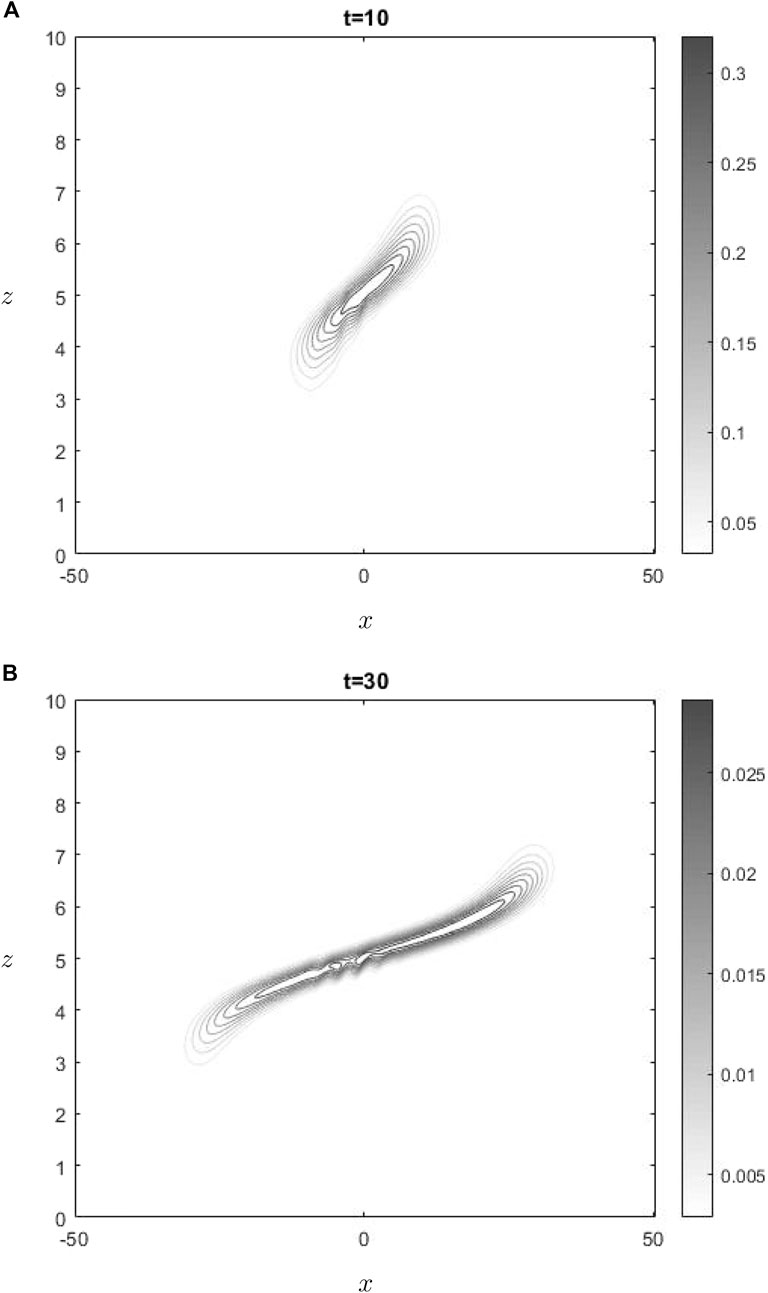
Figure 1. (A) represents
According to scientific literature, water vapor is widely recognized as the primary greenhouse gas inside the Earth’s atmosphere (Wallace and Hobbs, 2006). According to recent research, it has been shown that the impact of thermal emissions resulting from water vapor present in the atmosphere has the potential to amplify global warming, which is predominantly attributed to carbon dioxide
Given that our model focuses only on the interaction between water vapor, gravity waves, and ozone, and taking into account that water vapor and ozone are considered at different layers, the scaled water vapor equation can be represented following (Brasseur and Solomon, 1984) as
where
According to (Holton, 2004), the heating rate caused by water vapor in the atmosphere has the form
the constant
In regards to the characterization of the chemical distribution profile, we are referring to past observational studies. As an example (Gille and Lyjak, 1986; Gettelman et al., 2000) conducted a study on the atmospheric heating caused by several chemicals, such as ozone and water vapor. According to their findings, the initial profile of ozone and water vapor have distributions that seems to be localized at the equator in the horizontal direction and at a specific vertical level in the vertical direction. This suggests that the initial condition of the chemical can be specified in the form
where
The full nondimensional model for equations modelling gravity waves coupled with ozone Equation 1 and water vapor Equation 5 takes the form
where
We consider the domain to be the rectangular domain
where c. c. represents the complex conjugate; and
As shown by (Booker and Bretherton, 1967), the direction of wave propagation can be determined by examining the group velocity of the waves. The group velocity in two dimensions is defined by the vector
where
As detailed in (Almohaimeed, 2019) based on the discussion of (Booker and Bretherton, 1967), when the vertical component of group velocity is positive, the waves are travelling upward, whereas a downward-travelling wave corresponds to negative group velocity.
The upper boundary condition is defined so that the waves formed at
As previously mentioned, the critical level occurs When the phase speed of the wave is equal to the mean flow. We consider a configuration with background wind speed of the form
Chemical heating in (9) affects the energy of the atmosphere and hence affects the energy of gravity waves. Gravity waves affect the distribution of the chemical as can be seen in Equations 11, 12, where the advection speed of the chemical is modified by the gravity wave perturbations. These effects are shown in the numerical simulations in the next sections.
3 Methodology
In this section, we present a brief description of the numerical method, where we use the pseudo-spectral method in the horizontal direction and a finite-difference discretization in the vertical direction, to solve our model represented by Equations 7–12. We solve these equations on the two dimensional spatial domain
We enforce the conditions that
The initial conditions considered for the chemical mixing ratio in the case of ozone as well as water vapor satisfy the conditions
The form of these conditions for gravity waves as well as the chemical mixing ratio allow the use of the spectral method. The spectral method is a powerful method that is usually implemented models involving oscillatory solutions. To apply the spectral method, the functions
and similarly for the chemical mixing ratio
The corresponding inverse Fourier transforms of Equations 15–18 are
Taking the Fourier transform of Equations 7–12, by applying Equations 15–22 we obtain the transformed equations, which we solve using the fourth-order Adams–Bashforth method for the time discretization and a finite-difference discretization for derivatives in the vertical direction.
At each time step, the pseudo-spectral method is applied to approximate the Fourier transform the nonlinear terms. At each time step, we find the inverse Fourier transform for quantities involved in the nonlinear terms and compute the multiplication in the physical space. We then approximate the Fourier transform of the resulting product. To avoid expensive computations, we use the Fast Fourier Transform (FFT) in our computations. More details of the description of the numerical methods can be found in (Almohaimeed, 2019).
4 Results
The simulations are achieved by using the following selection of parameters. The velocity in the background is given by the hyperbolic tangent function
The initial values are considered as
The vertical extent of ozone is assumed to be between 0 and 60 km, whereas the horizontal dimension is defined as
According to the ozone distribution, as, in (Gille and Lyjak, 1986), ozone profile which exhibits a peak concentration at approximately 30 km altitude, may be represented by a Gaussian function as
where
In the case of water vapor, highest concentration is observed at around 15 km vertically and near the equator horizontally. Thus, the nondimensional initial form of water vapor can be considered as
where
The numerical simulations of the mathematical model with the initial profile of ozone represented by Equation 24 and initial profile of water vapor represented by Equation 25, are shown in the following set of figures.
5 Discussion
In this section we investigate the numerical solutions of the model obtained in the previous section. We also compare these numerical simulations with analytical observations obtained based on the equations of wave-induced mean streamfunction and density.
The graph shown in Figure 1 illustrates the temporal changes in ozone concentration, specifically highlighting gravity waves influence in the vicinity of the critical layer. Upon examining the development shown in Figure 1 at two different times, it becomes evident that there is a gradual decrease in ozone levels over time. The observed phenomenon may be expected, as shown by the negative coefficient of the first term in Equation 11. Consequently, the change in ozone concentration is directly proportional to the exponential decay function
The water-vapor concentration at two times is shown in Figure 2. In the lower region, where the concentration of water vapor is present, the dominant contribution to advection is attributed to the mean flow, whereas the effect of the advection resulting from gravity wave perturbations is relatively small. This phenomenon is present in Figure 2, wherein it can be seen that the concentration is undergoing advection towards the left, thereby departing from the active region of gravity waves interactions. This phenomenon does not apply to ozone, since it is situated precisely at the critical level. Consequently, ozone is transported towards the left when positioned below
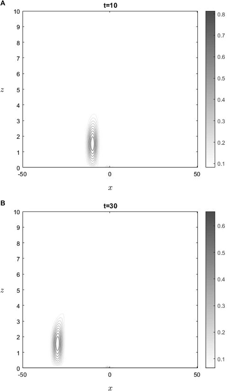
Figure 2. (A) represents
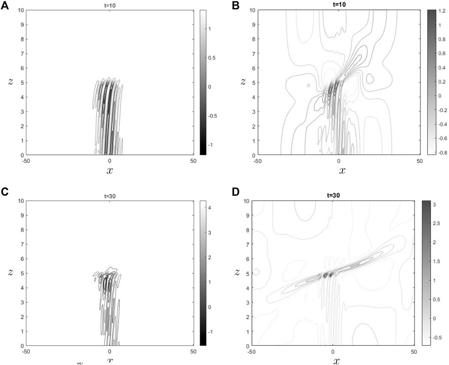
Figure 3. The sub Figures (A) and (C) show
Figures 3, 4 illustrate the impact of ozone and water vapor on the horizontal velocity and gravity waves density throughout both initial and final time periods. In both shown images, it is seen that the behavior of gravity waves in the vicinity of the critical level
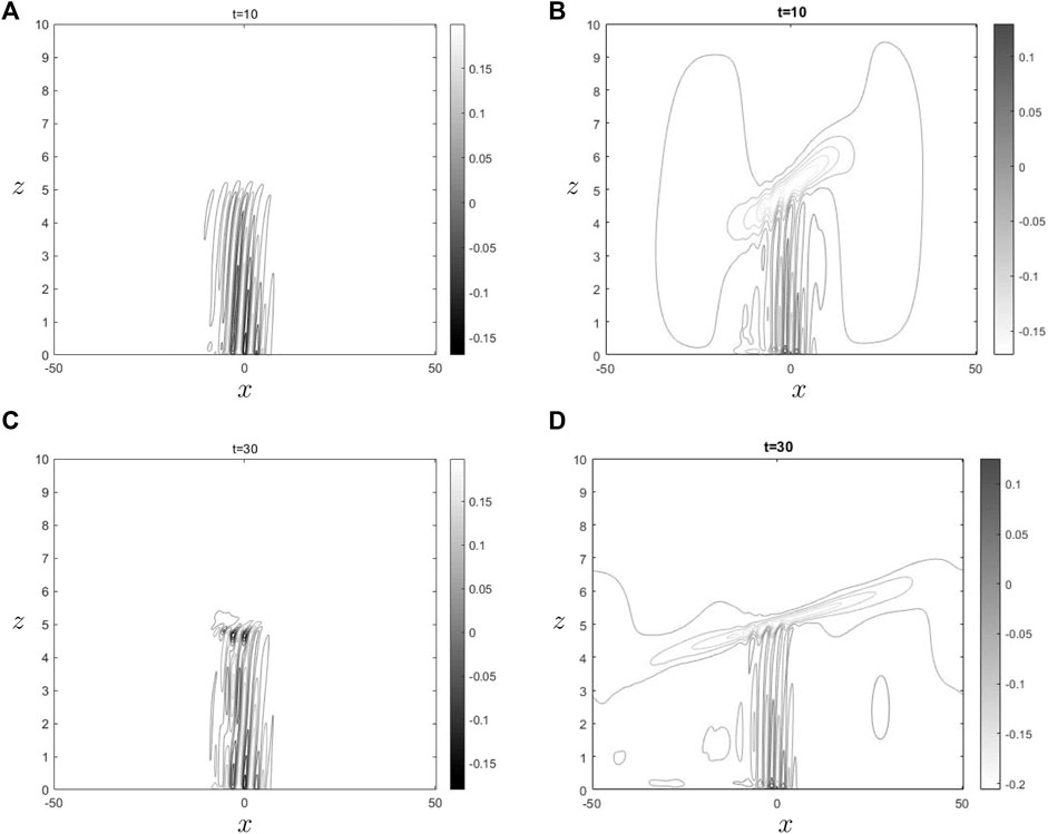
Figure 4. The sub Figures (A) and (C) show
The Fourier spectra of the streamfunction at the point
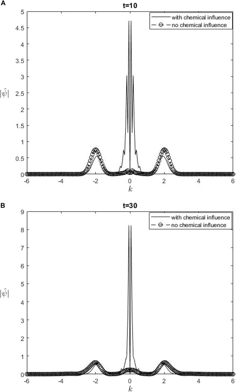
Figure 5.
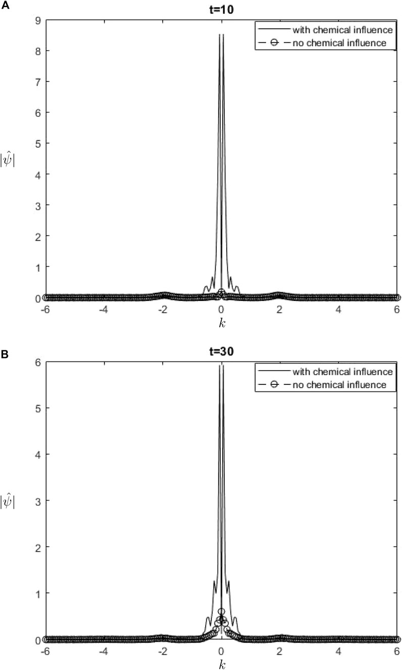
Figure 6.
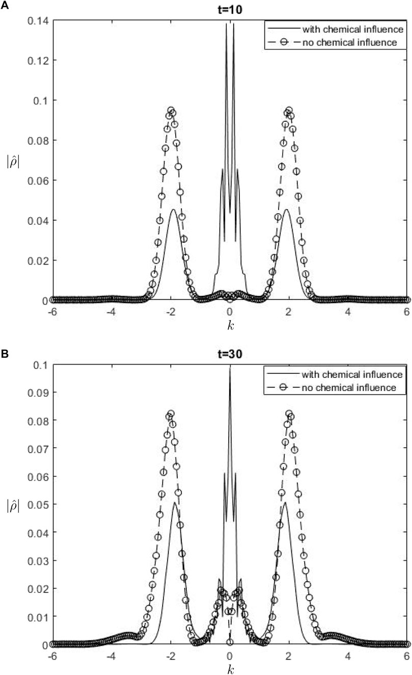
Figure 7.
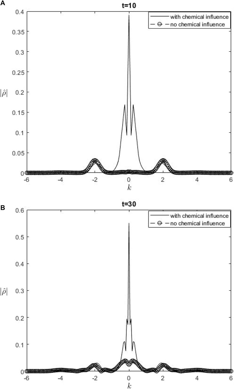
Figure 8.
When performing a comparison between the Fourier spectra of the streamfunction and that of density at the critical level, specifically at the zero wavenumber
whereas the mean flow induced from density, is given as
Equations 26, 27 may be utilized inside a parameterization framework. The equations presented include the influence of ozone and water vapor, allowing for the calculation of gravity-wave drag in scenarios where gravity waves interact with water vapor and ozone. It is important to acknowledge that although waves in our model are influenced by heating from the chemicals, the impact of such interaction is not evident in Equation 26. Consequently, there is no obvious influence of the chemical mixing ratio on the zero wave-number part of the Fourier streamfunction. In Equation 27, it is seen that the chemical forcing has an impact on the mean flow induced by density. This can be observed by examining the second and third terms on the right-hand side of Equation 27. Consequently, the density spectrum’s zero wavenumber component is influenced.
Overall, we note from the simulations that gravity waves impact the distribution of both ozone and water vapor via their induced vertical and horizontal movements, causing variations to the mixing ratio of these chemicals. The resulting variations in chemical concentrations cause modifications in the local temperature and density profiles as a result of energy absorption and release via photodissociation and latent heat activities. These thermal impacts alter the atmosphere buoyancy and stability, therefore affecting the propagation, amplitude, and phase speed of gravity waves. On the other hand, the existence of ozone and water vapor affects the temperature distribution in the atmosphere, leading to areas of varying heating that may either lead to the damping or enhancement of gravity waves.
6 Conclusion
The investigation focused on examining the dynamic interplay between gravity waves and ozone and water vapor inside the Earth’s atmosphere. Gravity waves were seen to have an impact on the genesis of ozone and water vapor. In contrast, the behavior of gravity waves is significantly influenced by the presence of ozone and water vapor, particularly in the vicinity of the critical threshold. Furthermore, it was shown that ozone and water vapor had an influence on the wavenumbers responsible for forcing, in addition to their impact on the zero wavenumber component.
Through numerical calculation, we have shown that the gravity wave equation has a significant impact on the advection of the mixing ratio of the chemical. Consequently, the wave-induced mean flow plays a substantial role in shaping the distribution of the chemical concentration. This phenomenon mostly manifests itself at the proximity to the critical threshold, when the mean flow caused by waves reaches its highest magnitude. The fluctuations of gravity waves induce disturbances in the chemical concentration, which ultimately exhibit the qualitative characteristics of the perturbations in gravity wave velocity. The impact of gravity wave fluctuations on the concentration of the chemical is consistent with the findings reported by (Garcia and Solomon, 1983; Xu et al., 2003).
The influence of chemical concentrations on gravity waves has been previously shown by (Leovy, 1966; Zhu and Holton, 1986; Xu, 1999). Nevertheless, the aforementioned research were grounded only on linear models. Additionally, the researchers took into account a consistent background mean flow, resulting in the absence of a critical threshold in their experimental setup. In our research, we took into account the whole nonlinear model of equations and included the mean flow that exhibits vertical shear, resulting in a configuration that includes a critical level. Our findings indicate that the non-linearity in the gravity waves equations and the existence of a critical level significantly impact the wave-induced mean flow. This effect becomes more pronounced as the waves propagate and the non-linearity intensifies, particularly in relation to chemical processes. The presence of non-linearity has a significant impact on the distribution of the chemical, resulting in a more pronounced effect. The chemical heating finally results in further impacts on gravity waves. Hence, the examination of gravity waves involving chemical constituents in the atmosphere is significantly influenced by both non-linearity and the presence of non-constant mean flow.
Data availability statement
The original contributions presented in the study are included in the article/Supplementary Material, further inquiries can be directed to the corresponding author.
Author contributions
AA: Conceptualization, Formal Analysis, Investigation, Methodology, Project administration, Resources, Software, Supervision, Validation, Visualization, Writing–original draft, Writing–review and editing.
Funding
The author(s) declare financial support was received for the research, authorship, and/or publication of this article. The Researchers would like to thank the Deanship of Graduate Studies and Scientific Research at Qassim University for financial support (QU-APC-2024-9/1).
Acknowledgments
The authors would like to thank the editors and anonymous reviewers for their valuable comments which helped to improve this project. The Researchers would like to thank the Deanship of Graduate Studies and Scientific Research at Qassim University for financial support (QU-APC-2024-9/1).
Conflict of interest
The author declares that the research was conducted in the absence of any commercial or financial relationships that could be construed as a potential conflict of interest.
Publisher’s note
All claims expressed in this article are solely those of the authors and do not necessarily represent those of their affiliated organizations, or those of the publisher, the editors and the reviewers. Any product that may be evaluated in this article, or claim that may be made by its manufacturer, is not guaranteed or endorsed by the publisher.
References
Almohaimeed, A. (2019). Internal-gravity-wave interactions in the presence of localized chemical heating in the atmosphere. Canada: Carleton University. Ph.D. thesis.
Booker, J. R., and Bretherton, F. P. (1967). The critical layer for internal gravity waves in a shear flow. J. Fluid Mech. 27, 513–539. doi:10.1017/s0022112067000515
Brasseur, G., and Solomon, S. (1984). Chemistry and physics of the stratosphere and mesosphere. Dordrecht, Netherlands: D. Reidel Publishing Company.
Brasseur, G. P., and Jacob, D. J. (2017). Modeling of atmospheric chemistry. Cambridge University Press.
Bretherton, F. P. (1966). Critical layer instability in baroclinic flows. Q. J. R. Meteorological Soc. 92, 325–334. doi:10.1002/qj.49709239302
Campbell, L., and Maslowe, S. (2003). Nonlinear critical-layer evolution of a forced gravity wave packet. J. Fluid Mech. 493, 151–179. doi:10.1017/s0022112003005718
Carpenter, L., Reimann, S., Burkholder, J., Clerbaux, C., Hall, B., Hossaini, R., et al. (2014). Scientific assessment of ozone depletion: 2014.
Dopplick, T. G. (1972). Radiative heating of the global atmosphere. J. Atmos. Sci. 29, 1278–1294. doi:10.1175/1520-0469(1972)029<1278:rhotga>2.0.co;2
Dopplick, T. G. (1979). Radiative heating of the global atmosphere: corrigendum. J. Atmos. Sci. 36, 1812–1817. doi:10.1175/1520-0469(1979)036<1812:rhotga>2.0.co;2
Garcia, R. R., and Solomon, S. (1983). A numerical model of the zonally averaged dynamical and chemical structure of the middle atmosphere. J. Geophys. Res. Oceans 88, 1379–1400. doi:10.1029/jc088ic02p01379
Gettelman, A., Holton, J. R., and Douglass, A. R. (2000). Simulations of water vapor in the lower stratosphere and upper troposphere. J. Geophys. Res. Atmos. 105, 9003–9023. doi:10.1029/1999jd901133
Gille, J. C., and Lyjak, L. V. (1986). Radiative heating and cooling rates in the middle atmosphere. J. Atmos. Sci. 43, 2215–2229. doi:10.1175/1520-0469(1986)043<2215:rhacri>2.0.co;2
Hartmann, D. L. (1994). Global physical climatology (international geophysics; v. 56). Academic Press.
Hickey, M. P., and Plane, J. (1995). A chemical-dynamical model of wave-driven sodium fluctuations. Geophys. Res. Lett. 22, 2861–2864. doi:10.1029/95gl02784
Holton, J. R. (2004). An introduction to dynamic meteorology, 88. Burlington, MA: Elsevier Academic Press.
Lacis, A. A., and Hansen, J. (1974). A parameterization for the absorption of solar radiation in the earth’s atmosphere. J. Atmos. Sci. 31, 118–133. doi:10.1175/1520-0469(1974)031<0118:apftao>2.0.co;2
Leovy, C. (1964). Radiative equilibrium of the mesosphere. J. Atmos. Sci. 21, 238–248. doi:10.1175/1520-0469(1964)021<0238:reotm>2.0.co;2
Leovy, C. B. (1966). Photochemical destabilization of gravity waves near the mesopause. J. Atmos. Sci. 23, 223–232. doi:10.1175/1520-0469(1966)023<0223:pdogwn>2.0.co;2
Lindzen, R. S., and Will, D. I. (1973). An analytic formula for heating due to ozone absorption. J. Atmos. Sci. 30, 513–515. doi:10.1175/1520-0469(1973)030<0513:aaffhd>2.0.co;2
London, J., and Park, J. H. (1974). The interaction of ozone photochemistry and dynamics in the stratosphere. a three-dimensional atmospheric model. Can. J. Chem. 52, 1599–1609. doi:10.1139/v74-232
Luther, F. M. (1976). A parameterization of solar absorption by nitrogen dioxide. J. Appl. Meteorology 15, 479–481. doi:10.1175/1520-0450(1976)015<0479:aposab>2.0.co;2
Marshall, J., and Plumb, R. (2008). Atmosphere, ocean, and climate dynamics: an introductory text, 93. Amsterdam: Elsevier Academic Press. [etc.].
Murgatroyd, R., and Goody, R. (1958). Sources and sinks of radiative energy from 30 to 90 km. Q. J. R. Meteorological Soc. 84, 225–234. doi:10.1002/qj.49708436103
Park, J. H., and London, J. (1974). Ozone photochemistry and radiative heating of the middle atmosphere. J. Atmos. Sci.31, 1898–1916. doi:10.1175/1520-0469(1974)031<1898:oparho>2.0.co;2
Shepherd, T. G. (2007). Transport in the middle atmosphere. J. Meteorological Soc. Jpn. Ser. II 85, 165–191. doi:10.2151/jmsj.85b.165
Strobel, D. F. (1978). Parameterization of the atmospheric heating rate from 15 to 120 km due to o2 and o3 absorption of solar radiation. J. Geophys. Res. Oceans 83, 6225–6230. doi:10.1029/jc083ic12p06225
Xu, J. (1999). The influence of photochemistry on gravity waves in the middle atmosphere. Earth, planets space 51, 855–861. doi:10.1186/bf03353244
Xu, J., Smith, A., and Ma, R. (2003). A numerical study of the effect of gravity-wave propagation on minor species distributions in the mesopause region. J. Geophys. Res. Atmos. 108. doi:10.1029/2001jd001570
Xu, J., Smith, A. K., and Brasseur, G. P. (2000). The effects of gravity waves on distributions of chemically active constituents in the mesopause region. J. Geophys. Res. Atmos. 105, 26593–26602. doi:10.1029/2000jd900446
Keywords: fluid mechanics, partial differential equations, computational fluid dynamics, heat transfer, gravity waves, atmospheric chemistry, ozone, water vapour
Citation: Almohaimeed AS (2024) Mathematical modelling for gravity waves interactions coupled with localized water vapor and ozone in the atmosphere. Front. Earth Sci. 12:1385305. doi: 10.3389/feart.2024.1385305
Received: 21 February 2024; Accepted: 16 July 2024;
Published: 02 August 2024.
Edited by:
Igo Paulino, Federal University of Campina Grande, BrazilReviewed by:
Petra Koucka Knizova, Institute of Atmospheric Physics (ASCR), CzechiaWenjun Dong, Global Atmospheric Technologies and Sciences, United States
Copyright © 2024 Almohaimeed. This is an open-access article distributed under the terms of the Creative Commons Attribution License (CC BY). The use, distribution or reproduction in other forums is permitted, provided the original author(s) and the copyright owner(s) are credited and that the original publication in this journal is cited, in accordance with accepted academic practice. No use, distribution or reproduction is permitted which does not comply with these terms.
*Correspondence: Ahmed S. Almohaimeed, YWhzLmFsbW9oYWltZWVkQHF1LmVkdS5zYQ==