Design and application of a monitoring device for embedded foundation side friction resistance

In geotechnical engineering, side friction resistance (SFR) is difficult to be measured directly. To further understand distribution law of the SFR, this paper developed a monitoring device that can directly measure the SFR. Further, a theoretical conversion formula for the elastic deformation and the SFR that considers the end effect of sensor sealing was proposed to guide the selection of sensor size and sealing material. Moreover, the monitoring device for the SFR was then calibrated using a large-scale direct shear apparatus and analyzed the stability of the sensor. The calibration results revealed that under cyclic loading and unloading conditions, the linear correlation coefficient of the sensor was greater than 0.996, and the sensitivity after sealing could reach 4.836 με/kPa, which met requirements of the engineering application. The developed monitoring device characterized by simple testing principle, low cost, and high precision were successfully applied to an open caisson project in Harbin City, which contributes to address the difficult problem of efficiently collecting the SFR in highways, bridges, water conservancy, and other projects.

1 Introduction

In geotechnical engineering, soil pressure and side friction resistance are important mechanical parameters, which have significant impacts on the study of soil mechanics and engineering practice. For example, the design and construction of embedded foundation, such as open caisson, caisson, and driven piles, all need to be based on accurate side friction resistance values (Tanimoto and Takahashi, 1994; Mitkina, 1996; Chakrabarti et al., 2006; Allenby et al., 2009; Ali and Madhav, 2013). However, it is difficult to directly monitor the SFR of submerged foundation, which makes it impossible to accurately capture the subsidence resistance during the construction process, which in turn prevents the controllable and efficient subsidence of embedded foundations from being realized. Compared with soil pressure sensors, attempts to directly test side friction resistance are limited. Stroud (Stroud, 1971) developed a device that can simultaneously monitor soil pressure and shear load. Although the device has a novel structure, there is a significant cross-effect between the monitored parameters, and it has rarely been used in engineering projects so far. More recently, Gan (Gan et al., 2018) has developed a shear stress sensor to monitor the shear strain at the interface between soil and structure, but the device remains in the laboratory stage due to unresolved waterproof sealing issues.

At present, scholars worldwide mainly adopt in-situ monitoring, laboratory test, numerical calculation, and theoretical analysis to study the SFR. In the field tests, New and Bowers (1994), Zhu et al. (2019), Yan et al. (2021) and Houlsby et al. (2006) obtained the SFR by multiplying the earth pressure on the side wall of a caisson by a certain friction coefficient through field monitoring. In addition, Pelecanos (Wang et al., 2019) and Wang et al. (Plecanos et al., 2017)used BOTDR and FBG respectively to measure the change value of axial stress of pile body to determine the average shear stress. Due to the indirect test method, there are certain errors in the actual SFR values, and the monitoring data are relatively discrete and poorly repeatable. This brings difficulties to theoretical analysis, and therefore many scholars have carried out laboratory experiments and numerical calculations.

In terms of laboratory tests, Tehrani (Tehrani et al., 2016) and Abidemi et al. (Olujide Ilori et al., 2017) concluded from laboratory model tests that normal pressure, concrete surface roughness, and soil compactness restricted the exertion of the SFR. Wang (Wang et al., 2013) and Mu (Mu et al., 2014) carried out sinking model tests of open caisson to investigate the change characteristics of side wall friction resistance, settlement range of soil surface outside the wall, and flow trend of soil particles when sinking the open caisson to different depths. Zhou et al. (2018) performed a series of laboratory centrifugal tests to study the distribution of the SFR under different caisson wall forms. Also, many scholars investigated the SFR of the embedded foundations through theoretical analysis. Yang et al. (2023) and Lai et al. (2022) proposed a calculation method for the SFR of the caisson during sinking, in which soil arch effect and stress relaxation effect of soil surrounding the caisson were considered. Based on the actual monitoring data of engineering projects, Li et al. (2023) and Dong et al. (2023) adopted the trained artificial neural network to predict soil parameters under different working conditions.

In summary, the studies on the SFR of embedded foundation have yielded remarkable achievements. Since the indirect test methods used in the field tests, laboratory tests, and theoretical analyses focus on a single soil layer or are simplified, and there are certain differences between test and actual SFR values (Sejia et al., 2014; Cao-Jiong et al., 2022). In order to solve the difficult problem of obtaining SFR directly, a new type of direct monitoring device for side friction resistance is proposed in this paper and applied in a caisson project in Harbin to verify the reliability of the device.

2 Structure design of the SFR sensor

For geotechnical tests such as triaxial test, ring shear test and direct shear test, the average shear stress of a characteristic shear surface represents the approximate shear stress at a point (Thermann et al., 2006). A shear stress sensor was developed based on the concept of the surface with points, which consisted of six parts: box, base, force transfer body, inverse column, S-shaped stress measurement unit, and sealing body (as illustrated in Figure 1). The S-shaped stress measurement unit was made of high elastic alloy, one end of which was fixed to the force transfer body through the reaction column 1, and the other end of which was fixed to the box through the reaction column 2. The two reaction columns could provide constraints for the S-shaped stress measurement unit. The box, base, and force transfer body were made of the stainless steel metal, while the sealing body adopted flexible waterproof sealing material. In addition, considering that the medium in contact with the soil affected the results of the SFR monitoring, a groove was set on the top of the force transfer body, which was filled with the same material as the measured medium.

Figure 1

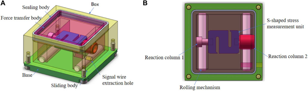
Figure 1. Three-dimensional structure diagram of the SFR sensor: (A) Three dimensional axonometry; (B) Cross-sectional view of the SFR sensor.

Since the SFR sensor was only sensitive to friction, it was not sensitive to positive pressure. Therefore, the key problem to be solved was the decoupling of the positive pressure and the SFR. To reduce the friction between the carrier and the base under the normal force, two decoupling methods, i.e., roller type and ball type, were designed in this study. Meanwhile, a gap was reserved between the carrier and the top of the box to prevent the contact between the force carrier and the box when the maximum shear force was applied.

3 Theory and simulation of the SFR sensor

3.1 Working principle

It was observed from Figure 2 that when the sensing surface was subjected to the SFR, the normal load was filtered by the sliding decoupling mechanism, and the force transfer body only transferred the SFR to the S-shaped stress measurement unit. Due to the constraint of the reaction pillar on the S-shaped stress measurement unit, the tension-and-compression stress sensor underwent a slight elastic deformation, causing strain recorded by the strain gauge. This in turn led to a change in the resistance of the strain gauge. The demodulation device detected the changes in the electrical signals and demodulated the corresponding side slip resistance value signals, thus achieving the measurement of the side slip resistance. However, there was an end effect at the contact point between the force transfer body and the sealing material under the influence of side slip resistance, which certainly affected the measured shear stress values. To elucidate the working mechanism of the sensor, it is necessary to study the structural mechanical characteristics of the S-shaped tension-and-compression sensor after taking into account the end effect generated by the sensor sealing.

Figure 2

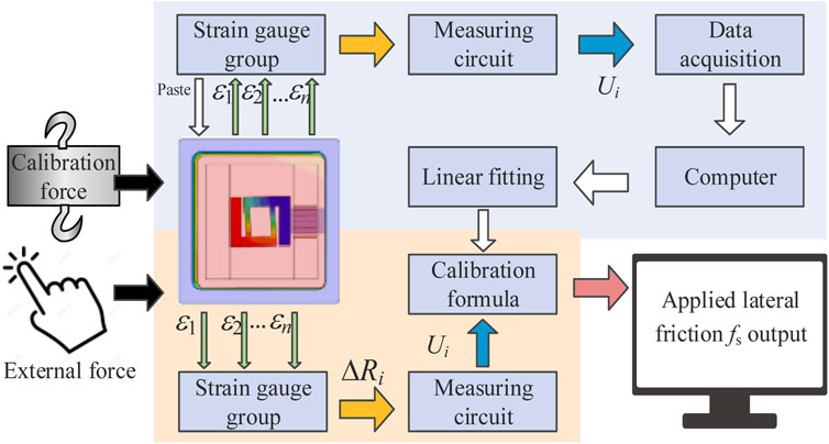
Figure 2. Schematic diagram of sensor working principle.

3.2 Analysis of elastic element forces

The elastic element in the side slip resistance sensor was a S-shaped load cell, with the upper strain gauges located in the same position as the cantilever beam structure (Figure 3A). For ease of calculation and analysis, the S-shaped load cell could be simplified to a closed framework structure with one end fixed and the other end acting as a cantilever (Geonea et al., 2020). In this simplified analysis, a concentrated force F and a counterclockwise bending moment of 0.5 FL were applied to the end of the upper balance beam. The structural mechanical model could be simplified to a single-span, three-degree-of-freedom statically indeterminated rigid framework, as indicated in Figure 3B.

Figure 3

Figure 3. S-shaped load cell and mechanical model: (A) S-shaped load cell and the placement of strain gauges; (B) Equivalent mechanical model.

To solve the three unknown forces, the following equations could be established (Hjelmstad, 2007):

$\left[\begin{array}{ccc}{\delta }_{11}& {\delta }_{12}& {\delta }_{13}\\ {\delta }_{21}& {\delta }_{22}& {\delta }_{23}\\ {\delta }_{31}& {\delta }_{32}& {\delta }_{33}\end{array}\right]\left[\begin{array}{c}{X}_1\\ X_2\\ X_3\end{array}\right]=-\left[\begin{array}{c}{\Delta }_{1\mathrm{P}}\\ {\Delta }_{2\mathrm{P}}\\ {\Delta }_{3\mathrm{P}}\end{array}\right](1)$

That was:

$\overline{\delta }\left\{X_i\right\}=-\left\{{\Delta }_{i\mathrm{P}}\right\}$

where δ_ij is the generalized displacement corresponding to X_i when X_i is the unit value; Δ_ip is the generalized displacement corresponding to X_i due to the load.

The displacement coefficients could be obtained using the method of graph multiplication:

$\overline{\delta }=\left[\begin{array}{ccc}\frac{H^{2}L}{2E{I}_{\mathrm{H}}}+\frac{H^3}{12E{I}_{\mathrm{V}}}& 0& 0\\ 0& \frac{2L^3}{3E{I}_{\mathrm{H}}}& -\frac{L^2}{E{I}_{\mathrm{H}}}\\ 0& -\frac{L^2}{E{I}_{\mathrm{H}}}& \frac{H}{E{I}_{\mathrm{V}}}+\frac{2L}{E{I}_{\mathrm{H}}}\end{array}\right](2)$

where I_H is the moment of inertia of the horizontal beam section; I_V is the moment of inertia of the vertical beam section, and E is the elastic modulus of the sensor material; L is the length of the horizontal balance beam; H is the length of the vertical beam.

$\left\{{\Delta }_{i\mathrm{P}}\right\}={\left[0,-\frac{F{L}^3}{12E{I}_{\mathrm{H}}},0\right]}^{\mathrm{T}}(3)$

By substituting Eqs 2, 3 into Eq. 1, the following equation could be obtained:

$\left\{X_i\right\}={\left[0,-\frac{F}{2}+\frac{3}{8+4K}F,-\frac{FL}{4}+\frac{2L}{8+4K}F\right]}^{\mathrm{T}}(4)$

where K = LI_V/HI_H.

By substituting the Eq. 4, the bending moment diagram of the S-shaped load cell could be solved. The bending moment at the ends of the parallel beam was given by:

$\begin{array}{l}{M}_1=M_3=\frac{FL}{4}+\frac{2FL}{8+4K}\\ M_2=M_4=-\frac{FL}{4}-\frac{FL}{8+4K}\end{array}(5)$

According to Eq. 5, the maximum bending stress and strain at the ends of the parallel beam were:

$\begin{array}{l}{\epsilon }_1={\epsilon }_3=-\frac{3FL}{2Eb{h}^2}-\frac{3FL}{\left(4+2K\right)Eb{h}^2}\\ {\epsilon }_2={\epsilon }_4=\frac{3FL}{2Eb{h}^2}+\frac{3FL}{\left(2+K\right)Eb{h}^2}\end{array}(6)$

The vertical beam I_V was much larger than the horizontal beam I_H, i.e., K was large. Eq. 6 was arranged as:

${\epsilon }_1={\epsilon }_3=-{\epsilon }_2=-{\epsilon }_4=-\frac{3FL}{2Eb{h}^2}(7)$

where b and h are the width and thickness of the horizontal balance beam, respectively.

The strain of the elastic element was converted into a change in the resistance to monitor the strain generated in the S-shaped load cell subjected to force. Also, to improve the sensitivity of the sensor and to eliminate the influence of temperature, four strain gauges were connected to form a resistance-strain full bridge (Arshak et al., 1997). The conversion principle of this sensor is displayed in Figure 4.

Figure 4

Figure 4. Schematic diagram of the SRF sensor strain gauge adhesive and circuit: (A) Sensor strain gauge adhesive; (B) Wheatstone bridge circuit.

The output voltage of the full bridge was given by:

$U_0=\frac{\left(R_1+\Delta R_1\right)\left(R_3+\Delta R_3\right)-\left(R_2-\Delta R_2\right)\left(R_4-\Delta R_4\right)}{\left(R_1+R_2+\Delta R_1-\Delta R_2\right)\left(R_3+R_4+\Delta R_3-\Delta R_4\right)}{U}_{\mathrm{S}}(8)$

where the U_s is the supply voltage; U₀ is the output voltage, R₁=R₂=R₃=R₄. By substituting the relation between resistance and strain into Eq. 8, U₀ can be rewritten as:

$U_0=\frac{1}{4}G\frac{{\epsilon }_1+{\epsilon }_3-{\epsilon }_2-{\epsilon }_4}{\left[1+\frac{1}{2}\left({\epsilon }_1+{\epsilon }_2+{\epsilon }_3+{\epsilon }_4\right)\right]}{U}_{\mathrm{S}}(9)$

where ε_j is the micro-strain of the strain gauge.

By rearranging the Eq. 9 the relationship between the SFR and the output voltage can be obtained:

$f_s=\alpha \frac{2Eb{h}^2}{3L}\frac{U_0}{AG{U}_S}(10)$

where the f_s is the SFR; A is the sensing area of the SFR sensor; and α is the end effect coefficient. The Eq. 10 reflects that the sensor sensitivity is related to the elastic beam size and material.

To verify the rationality of the derived formula for S-shaped load cell, this study utilized ABAQUE software to calculate and analyze the maximum strain at the end of the balanced beam with beam lengths of 12 mm, 14 mm, and 16 mm as well as different beam thicknesses h. The sensor chosen for analysis had a Young’s modulus of 200 GPa and a Poisson’s ratio of 0.3. A load of 1000 N was applied to the sensor. It was observed from Figure 5 that the theoretical calculation results of the maximum strain at the beam end matched well with the finite element simulation results, which verified the reasonableness of the derived theoretical formula.

Figure 5

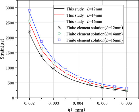
Figure 5. Comparison between theoretical solution and numerical simulation results.

4 Determination of sensor size and sealing material

4.1 Selection of sensor size

The sizes of sensor were selected with the main consideration of facilitating the convenient layout, so that it could be installed between the longitudinal main ribs. The spacing between the steel bars in the field typically ranged from 12 cm to 20 cm. Therefore, the sizes of the sensor were determined to be 10 cm (length)×10 cm (width) ×6 cm (height). The sensing area on the SFR surface were determined to be 7.0 cm long and 7.0 cm wide (Figure 6).

Figure 6

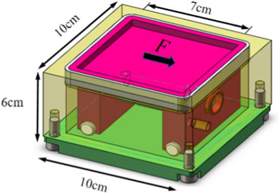
Figure 6. The SFR Sensor external profile dimensions.

To satisfy the range requirements for monitoring the SFR in large-scale sinking foundations, the maximum measurement range of the SFR device was set to 200 kPa. Based on the sensing area (49 cm²), the maximum tension and compression force on the strain gauge was calculated to be 980 N. According to Eq. 7, the relationships between the balanced beam length, thickness, and the strain as well as maximum stress at the end of beam under a SFR of 200 kPa are illustrated in Figure 7. It was observed that as the thickness of the parallel beam decreased and the length increased, the strain of the elastic element under the load increased, indicating a more sensitive sensor. However, the maximum tension and compression stress σ_max also increased, which might cause the sensor to reach the yielding state. To meet the high-precision requirements for the sensor with a large measurement range, the parameters of the elastic element were determined, as summarized in Table 1. The S-shaped stress measurement unit and the SFR sensor were made of stainless steel, and their physical appearances are displayed in Figure 8.

Figure 7

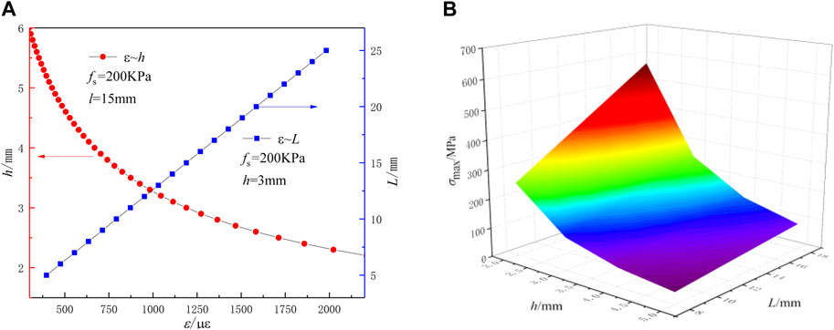
Figure 7. The relationship between strain and maximum stress of balance beam and h and L: (A) The relationship between ε and h, L; (B) The relationship between σ_max and h, L.

Table 1

Table 1. Dimension parameters of tension and pressure sensors.

Figure 8

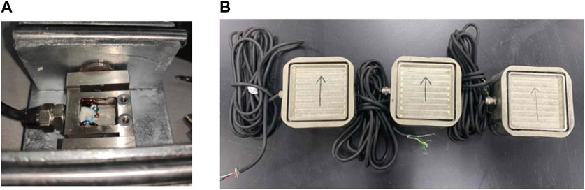
Figure 8. The S-shaped load cell and the SRF sensor: (A) S-shaped stress measurement unit; (B) The SRF sensor.

4.2 Selection of sealing material

The SFR sensor in geotechnical engineering is always exposed to the environment of high water and soil pressures that require sealing. However, the sealing will produce end effect on the force transfer body and affect the test results. In order to reduce the strain loss of the S-shaped stress measurement unit after the sealing of SFR sensor, it is necessary to analyze the force of the sensor to provide guidance for the selection of sealing material. Although the strain loss caused by the end effect can be compensated by the laboratory calibration test, the sensitivity of the sensor will be reduced if the strain loss is too large. Due to the constraint effect of the sealing body on the force transfer body after the sensor is sealed, the force of the sensor is relatively complicated and the traditional analytical algorithm cannot capture the mechanical characteristics of the elastomer well. Therefore, the finite element method was utilized to simulate the working condition of the sensor to make up for the shortage of theoretical analytical calculation.

In this section, the ABAQUS finite element software was employed to establish a finite element analysis model of the SFR sensor in Figure 9. The S-shaped load cell in the sensor was fixed inside the housing by a reaction column. Therefore, both the elastic body and the reaction column were constrained. In addition, the bottom of the force transfer body was a sliding mechanism that allows tangential displacement. Therefore, the bottom of the force transfer body was only constrained for normal displacement. Since the lateral force transfer was influenced by both the elastic body and the sealing material, the stress characteristics of the sensor were related to the ratio of the elastic modulus of the sealing material to the elastic modulus of the elastic body (E_g/E_s). In this case, the elastic body of the sensor was an elastic structure. Based on the principle of virtual work (Craig and Taleff, 2020), the formula for calculating the equivalent modulus, E_g of the sensor can be solved in Eqs 11a, b:

${\Delta }_{\mathrm{g}}=\int \frac{{\overline{M}}^{2}ds}{E{I}_{\mathrm{H}}}=\frac{L^3}{24E{I}_{\mathrm{H}}}(\mathrm{11a})$

$E_{\mathrm{g}}=\frac{1}{{\Delta }_{\mathrm{g}}}=\frac{2Eb{h}^3}{L^3}(\mathrm{11b})$

where Δ_g is the horizontal displacement of the SFR sensor under the action of unit force; $\overline{M}$ is the sectional bending moment of the S-shaped force measurement unit under a unit force. Six working conditions were numerically calculated to analyze the influence of the strain transfer coefficient of the sensor under different modulus ratios, as listed in Table 2.

Figure 9

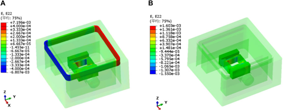
Figure 9. Finite element analysis results of SRF sensor with different modulus ratios at side friction resistance of 200 kPa: (A) Es/Eg = 0.25; (B) Es/Eg = 0.

Table 2

Table 2. Numerical calculation conditions.

Figure 10 displays the relationship between the modulus ratio of the elastic body and the sealing material as well as the strain ratio. It was observed that the strain at the beam end of the parallel beam of the S-shaped load cell without any sealing material was 1,216 uε. As the elastic modulus of the sealing material (E_s), i.e., the ratio E_s/E_g increased, the maximum strain at the beam end of the parallel beam gradually decreased. In case of E_s/E_g=0.0125 (i.e., E_s=0.5 MPa), the strain of the parallel beam was 0.9 times that without sealing material, demonstrating a 10% strain loss after sealing. In case of E_s/E_g=0.025 (i.e., E_s=1.0 MPa), the strain loss after sealing was 19%. This loss increased until E_s/E_g=0.25 (i.e., E_s=10 MPa), where the strain loss after sealing reached 65%. Therefore, it is crucial to select an appropriate sealing material to minimize the loss of sensitivity of the sensor.

Figure 10

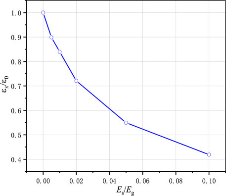
Figure 10. Relation curves of different stiffness ratios and strains.

The commonly used sealing materials and their parameters are illustrated in Table 3. It was observed from the numerical calculation results that the strain loss after sealing with a rubber ring (E_s=7.8 MPa) varied from 50% to 65%. However, the strain loss was only 10% when a silicone structural adhesive (E_s=0.5 MPa) was used for sealing. Hence, the selection of a silicone structural adhesive with a lower elastic modulus had the least impact on sensor sensitivity.

Table 3

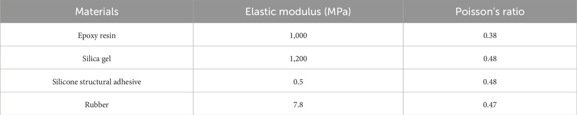
Table 3. Commonly used sealing materials and parameters.

5 Sensor calibration and stability analysis

5.1 Testing equipment and scheme

The calibration system was designed and modified on the basis of a large-scale direct shear apparatus to realize the graded loading calibration of the SFR sensor. As displayed in Figure 11A, the SFR sensor calibration system consisted of the large-scale direct shear apparatus, the SFR sensor, the sensor transmitter, the signal transmission line, the straight shear apparatus control system, and the signal acquisition system.

Figure 11

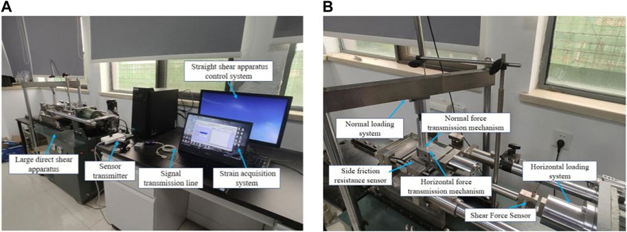
Figure 11. Calibration system of the SFR sensor: (A) Calibration system composition; (B) Calibration system force transmission mechanism.

Considering that the calibration of the SFR sensor needed to verify the validity of the decoupling of the positive pressure and the SFR of the sensor, the normal and horizontal force transfer mechanisms were designed on the basis of the large-scale direct shear instrument, and the force transfer ends were embedded in the sensor groove to realize the quantitative loading of normal and horizontal forces (Figure 11B). The loading was controlled by servo motor with constant shear force.

5.2 Analysis of test results

5.2.1 Comparison of decoupling methods

The sensors were calibrated using two methods to compare the effect and stability of the two decoupling methods. Three normal pressures of 50 kPa, 100 kPa, and 200 kPa were applied to each set of tests to obtain the corresponding sensitivity coefficients C₁, C₂, and C₃ for the SFR sensor.

As revealed in Figure 12, the calibration curves of both decoupling methods exhibited obvious linear characteristics, and the loading curves under different normal stresses were in good agreement. In addition, the sensitivity coefficient decreased with the increase of the normal force, indicating that the balls or rollers inside the sensor generated friction under the normal force.

Figure 12

Figure 12. Calibration curves of the SFR sensor under different normal forces: (A) Roller decoupling method; (B) Ball decoupling method.

The test results showed that the correlation coefficient of the sensor calibration curve obtained by the roller decoupling method was 0.995, and the average sensitivity coefficient of the sensor was 5.059 με/kPa. The correlation coefficient obtained by the ball decoupling method was 0.998, and the sensitivity coefficient was 5.267 με/kPa. Therefore, the calibration curve of the SFR sensor obtained using the ball decoupling method had better linear correlation and higher sensor sensitivity. The ball decoupling method would be used for the follow-up study.

In addition, to examine the filtering effectiveness of the SFR sensor against the normal load of the panel, the SFR of the sensor subjected only to vertical pressure was observed. As demonstrated in Figure 13, the normal force-SFR curves of the two SFR sensors were essentially parallel to the horizontal axis. The roller sensor was slightly more affected by the normal force compared with the ball sensor, but in general the SFR was close to 0 kPa for different vertical pressures. This indicated that both decoupling methods were effective in filtering the interference of the normal force perpendicular to the sensor panel.

Figure 13

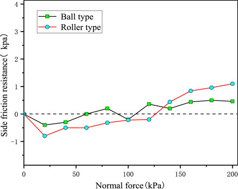
Figure 13. Curve of the SFR versus normal force under horizontal load of 0 kPa.

5.2.2 Comparison of performance before and after sealing

Figure 14 displays the sensor calibration curves before and after sealing. The cyclic loading and unloading process basically overlapped and exhibited obvious linear characteristics. The fitting sensitivity coefficients before and after sealing were 5.194 με/kPa (R² =0.997) and 4.836 με/kPa (R² =0.996), respectively. Comparison of the sensitivity coefficients before and after sealing revealed that some of the SFR would be lost when the sealing material was filled between the force transfer body of the SFR sensor and the box, resulting in a certain decrease in the sensitivity of the sensor.

Figure 14

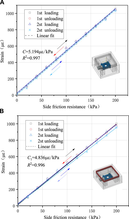
Figure 14. Calibration curves before and after sealing of the SFR sensor: (A) Sensor calibration curve before sealing; (B) Sensor calibration curve after sealing.

The loss rate of sensitivity after sealing was calculated to be 8.5% (numerically calculated to be 10%). Therefore, the SRF sensor response considering the sealing effect could be expressed as follows:

$f_s=\frac{\epsilon }{C}(12)$

where C is calibration factor after sealing, with a value of 4.836 με/kPa. According to Eq. 12, the sensor strain can be converted into the side friction resistance.

5.2.3 Sealing performance test

To test the sealing effect of the SFR sensor, the sensor was immersed in a sealed container filled with water (Figure 15A), then the pressure inside the container was increased to 0.7 MPa by an air compressor, and the sensor was continuously tested for 1 month at this pressure. Figure 15B displays the strain curve of the sensor during the 30-day sealing test. The test results confirmed that the sensor could work normally under high water pressure condition and had good sealing and waterproof performance.

Figure 15

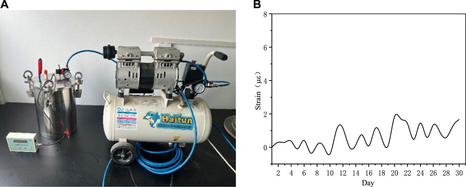
Figure 15. Sealing performance test of the SFR sensor: (A) Sensor sealing performance test; (B) Strain curve of the sensor during the sealing test.

6 Project application

6.1 Test condition and sensor position

To evaluate performance of the SFR sensor, a field test was conducted on the pipe-jacking receiving well of the No. 1 open caisson of a wastewater treatment plant in Harbin City. The open caisson had a diameter of 17 m, a height of 32.35 m, and a wall thickness of 1.5–1.8 m. A top-to-bottom distribution of soil layers is displayed in Table 4. The groundwater in the open caisson site was pore diving. The depths of the initial groundwater level and the static water level were 0.00–0.96 m and 0.00–0.69 m, respectively.

Table 4

Table 4. Distribution of engineering geological layer.

In the field test, two monitoring sections were selected from the side wall of the open caisson. Three earth pressure boxes (ET) and three SFR monitoring devices (FT) were installed in each monitoring section, and their distances from the edge of the open caisson were 1 m, 6 m, and 11 m, respectively, as displayed in Figure 16A. The earth pressure boxes and the SFR monitoring devices were installed at the same elevation of the shaft wall, with a transverse distance of 40 cm. The data from the two sensors were transmitted to the ground signal transmitting module via the acquisition module, and then they were uploaded to the cloud platform through the signal transmitting module to enable data monitoring and storage. In addition, the sinking depth and plane deviation of the caisson were regularly monitored by the total station. Abidemi Olujide Ilori et al. (Olujide Ilori et al., 2017) stated that the surface material and roughness of the structure were crucial factors affecting the friction coefficient of soil-structure interface. Therefore, the SFR sensors were embedded in the outer wall of the open caisson, and their sensing surface should be flush with the sunken wall. The groove of the sensing surface should be filled with cement mortar to ensure that the roughness of the contact interface of the sensors were consistent with that of the sunk wall. The field installation is presented in Figures 16B, C.

Figure 16

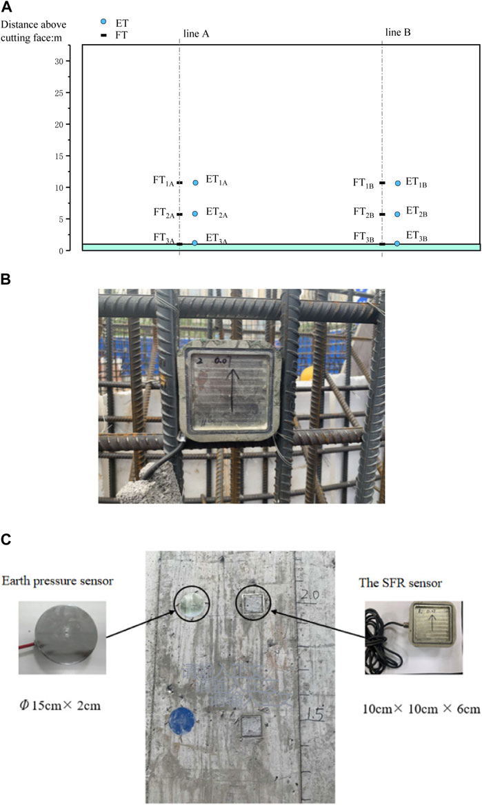
Figure 16. The SRF sensor deployed in the field: (A) Monitoring instrument layout diagram; (B) Sensor fixed to steel rebar prior to casting of the concrete walls; (C) Sensor exposed surface after casting.

6.2 Monitoring results

6.2.1 Overall sinking

As shown in Figure 17A, the sinking of the open caisson began on 28 April 2022 and reached the design elevation on 26 August 2022, with a cumulative sinking depth of 32.5 m. The average sinking speed was about 0.33 m/d, with the fastest sinking speed of 2 m/d. The sinking speed was faster in sandy soil layers and relatively slower in cohesive soil layers. As shown in Figure 17B, x-x and y-y were two mutually orthogonal coordinate axes. It was observed that the deviation of the open caisson during the initial sinking stage was quite drastic. However, as the depth of the open caisson increased, the surrounding soil provided a stronger constraint on the open caisson, and the inclination of the open caisson only changed slightly. This highlighted the importance of ensuring that the open caisson was in excellent condition during the initial sinking stage.

Figure 17

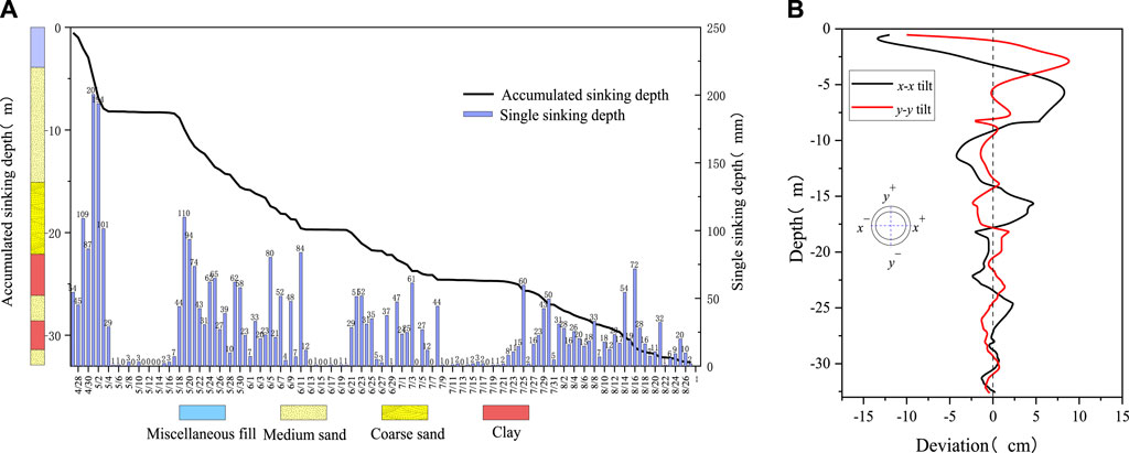
Figure 17. Overall sinking of the open caisson: (A) Sinking curve; (B) Deviation curve.

6.2.2 Sensor monitoring results

The lateral pure earth pressure ${\sigma }_{\mathrm{n}}^{\prime }$ on the side wall of open caisson is obtained by subtracting water pressure from the earth pressure sensors, which can be calculated from Eq. 13a.

${\sigma }_{\mathrm{n}}^{\prime }={\sigma }_{\mathrm{n}}-p(\mathrm{13a})$

where σ_n is the total normal stresses measured by individual ETs; and p is the fluid pressure.

The variation of lateral pure earth pressure with depth is shown in Figure 18, which indicated that the lateral earth pressure increased with the increase of depth. When the open caisson attitude changed greatly, the lateral earth pressure on the measured wall varied between the passive earth pressure and the active earth pressure, which led to drastic change of the lateral earth pressure. In the late sinking stage, the open caisson attitude tended to be stable, and the lateral earth pressure values from the earth pressure sensors at the same depth were close to each other.

Figure 18

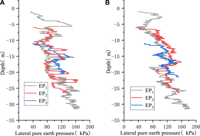
Figure 18. Lateral pure earth pressure vs. soil depth: (A) Results of monitoring line A; (B) Results of monitoring line B.

The SFR of the open caisson could be acquired by the monitoring device buried at the site. The monitoring results of the SFR in Figure 19 revealed that the SFR of the side wall of the open caisson varied between 0 and 60 kPa, which was the same as the fact that the earth pressure increases with the increasing soil depth. It was also observed that the fluctuation of the SFR test results was basically consistent with that of the soil pressure test results, which verified the reliability of the monitoring results of the SFR device.

Figure 19

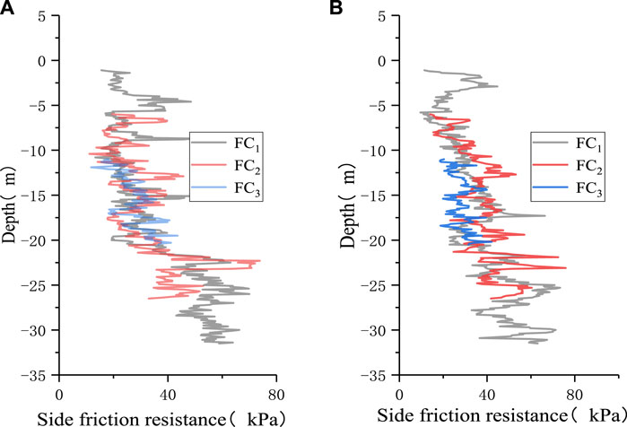
Figure 19. Curves of side friction vs. soil depth: (A) Results of monitoring line A; (B) Results of monitoring line AB.

The friction resistance between caisson and soil mainly depends on the friction coefficient δ at the soil-concrete interface, which can be calculated from Eq. 13b:

$\delta ={\tan }^{-1}\left(\frac{f_{\mathrm{s}}}{{\sigma }_{\mathrm{n}}^{\prime }}\right)(\mathrm{13b})$

where f_s is the shear stresses measured by individual FCs.

The variation of interface friction coefficient with depth is shown in Figure 20, where the tanδ at the concrete interface is also plotted for comparison (Potyondy, 1961). It was observed that the interface friction coefficient δ for sand-concrete and clay-concrete were 0.6 ${\phi }^{\prime }$-0.7 ${\phi }^{\prime }$ and 0.8 ${\phi }^{\prime }$-0.9 ${\phi }^{\prime }$, respectively. However, Potyondy conducted a large number of direct shear tests to study the shear tests between various soils and structural interfaces, and found that the interface friction coefficients for sand-concrete and clay-concrete were 0.9 ${\phi }^{\prime }$ and ${\phi }^{\prime }$, respectively. The reason for this is that the sinking of caisson causes the surrounding soil to become looser, and the friction interface of groundwater infiltration also leads to a decrease in the interface friction coefficient. Therefore, the friction coefficient from direct shear test for the construction of caisson will overestimate the side friction resistance. It is necessary to use direct test method to obtain the SFR for the design and construction of embedded foundation.

Figure 20

Figure 20. Variation of interface friction angle with depth: (A) Results of monitoring line A; (B) Results of monitoring line B.

7 Conclusion

A monitoring device that can directly collect the SFR was developed to address the problem of difficulty and low accuracy in capturing the SFR during the construction of sinking foundations. Sensitivity analysis was carried out on parameters such as sensor structure size and sealing material properties through sensing theory and numerical simulation analysis methods. A SFR test method was established through the sensing theory analysis and the laboratory calibration experiment, and field tests were carried out in caisson projects. The main work and research results carried out in this paper were as follows:

(1) A monitoring device for directly acquiring the SFR was proposed. The S-shaped force measurement unit was simplified into a closed frame structure, and the theoretical conversion formula for the strain and the SFR of the sensor was derived. The rationality of the theoretical derivation formula was verified by comparing with the numerical simulation results. Based on the sensitivity analysis of the sensor structure size parameters, the sizes of S-shaped stress measurement unit of L = 15 mm, b = 10 mm, h = 3 mm were determined.

(2) The ratio of the equivalent modulus of the S-shaped force measurement unit to the modulus of the sealing material affected the sensitivity of the SFR sensor. As the modulus ratio increased, the strain at the end of the balance beam gradually decreased, i.e., the strain loss increased. When a silicone structure (E_s=0.5 MPa) was utilized for sealing, the strain loss was 10%, which had a relatively small impact on the sensitivity of the sensor.

(3) The calibration results showed that the two decoupling methods could filter out the influence of normal stress on the test results, and the ball decoupling method exhibited higher sensitivity. After sealing the calibration results of the SFR sensor indicated that there was a good overlap during the loading and unloading processes within the measurement range, with a linear correlation coefficient R² greater than 0.996 and a sensitivity coefficient of 4.885 με/kPa. The SFR sensor was able to work continuously and stably under 0.7 MPa water pressure environments, which satisfied meeting the requirements of engineering applications.

(4) The high survival rate of the SFR sensor in field applications was corroborated by its monitoring results, which demonstrate that the SFR increases with the increase of soil depth and the fluctuation of SFR test values are basically consistent with that of earth pressure test values, thus verifying the reasonableness of the monitoring results from the SFR device.

(5) The friction coefficient from direct shear test for the construction of caisson will overestimate the side friction resistance. It is necessary to use direct test method to obtain the SFR for the design and construction of embedded foundation.

Data availability statement

The original contributions presented in the study are included in the article/Supplementary Material, further inquiries can be directed to the corresponding author.

Author contributions

WT: Writing–original draft, Funding acquisition. PC: Conceptualization, Writing–review and editing. JL: Conceptualization, Methodology, Writing–review and editing. FJ: Investigation, Supervision, Writing–review and editing.

Funding

The author(s) declare that financial support was received for the research, authorship, and/or publication of this article. National key Research and Development Program of China 2022YFB2302500.

Conflict of interest

Authors WT, PC, JL, and FJ were employed by CCCC Second Harbor Engineering Company, Ltd.

Publisher’s note

All claims expressed in this article are solely those of the authors and do not necessarily represent those of their affiliated organizations, or those of the publisher, the editors and the reviewers. Any product that may be evaluated in this article, or claim that may be made by its manufacturer, is not guaranteed or endorsed by the publisher.

References

Ali, J. S. M., and Madhav, M. R. (2013). Analysis of axially loaded short rigid composite caisson foundation based on continuum approach. Int. J. geomechanics 13 (5), 636–644. doi:10.1061/(asce)gm.1943-5622.0000185

CrossRef Full Text | Google Scholar

Allenby, D., Waley, G., and Kilburn, D. (2009). Examples of open caisson sinking in Scotland. Proc. Institution Civ. Engineers-Geotechnical Eng. 162 (1), 59–70. doi:10.1680/geng.2009.162.1.59

CrossRef Full Text | Google Scholar

Arshak, K. I., Ansari, F., McDonagh, D., and Collins, D. (1997). Development of a novel thick-film strain gauge sensor system. Meas. Sci. Technol. 8 (1), 58–70. doi:10.1088/0957-0233/8/1/009

CrossRef Full Text | Google Scholar

Cao-Jiong, L., Huang, R., and Yuan-Gang, M. (2022). Researchon caisson sinking resistance in clay-sand intersected stratum. Bridge Constr. 52 (04), 61–67. doi:10.3969/j.issn.1003-4722.2022.04.009

CrossRef Full Text | Google Scholar

Chakrabarti, S. K., Chakrabarti, P., and Krishna, M. S. (2006). Design, construction, and installation of a floating caisson used as a bridge pier. J. Waterw. port, Coast. ocean Eng. 132 (3), 143–156. doi:10.1061/(asce)0733-950x(2006)132:3(143)

CrossRef Full Text | Google Scholar

Craig, R. R., and Taleff, E. M. (2020). Mechanics of materials. John Wiley & Sons.

Google Scholar

Dong, X., Tu, J., Xu, J., Cai, L., Wu, B., and Cai, L. (2023). “Based on Abaqus finite element analysis software to assist the construction of super large caisson,” in 2023 international Seminar on computer Science and engineering Technology (SCSET) (IEEE), 627–631.

CrossRef Full Text | Google Scholar

Gan, F., Ye, X., Yin, K., Li, M., Yang, J., and Xiao, Y. (2018). Experimental study on progressive failure of soil-structure interfaces based on a new measuring method of local stress and displacement. Chin. J. Rock Mech. Eng. 37 (3), 734–742. doi:10.13722/j.cnki.jrme.2017.0781

CrossRef Full Text | Google Scholar

Geonea, I. D., Dumitru, N., Margine, A., Craciunoiu, N., and Copiluși, C. (2020). Design, manufacture and testing of a S type force transducer. Appl. Mech. Mater. 896, 255–262. doi:10.4028/scientific.net/amm.896.255

CrossRef Full Text | Google Scholar

Hjelmstad, K. D. (2007). Fundamentals of structural mechanics. Springer Science & Business Media.

Google Scholar

Houlsby, G. T., Kelly, R. B., Huxtable, J., and Byrne, B. W. (2006). Field trials of suction caissons in sand for offshore wind turbine foundations. Géotechnique 56 (1), 3–10. doi:10.1680/geot.2006.56.1.3

CrossRef Full Text | Google Scholar

Lai, F., Liu, S., and Deng, Y. (2022). Research progress on mechanical characteristics and environmental effects of Construction process of giant deep buried caisson. Chin. J. Basic Eng. Sci. 30 (03), 657–672. doi:10.16058/j.issn.1005-0930.2022.03.012

CrossRef Full Text | Google Scholar

Li, Z. L., Zhang, X., Dai, G., and Cao, S. (2023). Study on soil parameter evolution during ultra-large caisson sinking based on artificial neural network back analysis. Sustainability 15, 10627. doi:10.3390/su151310627

CrossRef Full Text | Google Scholar

Mitkina, G. V. (1996). Bearing capacity of hollow piles sunk in leader holes. Soil Mech. Found. Eng. 33 (3), 105–108. doi:10.1007/bf02361020

CrossRef Full Text | Google Scholar

Mu, B. G., Bie, Q., Zhao, X. L., and Gong, W. M. (2014). Meso-experiment on caisson load distribution characteristics during sinking. China J. Highw. Transp. 27 (09), 49–56. doi:10.19721/j.cnki.1001-7372.2014.09.007

CrossRef Full Text | Google Scholar

New, B. M., and Bowers, K. H. (1994). “Ground movement model validation at the Heathrow Express trial tunnel,” in Tunnelling’94 (Boston, MA: Springer), 310–329. Proceedings of the 7th International Symposium IMM and BTS, London.

CrossRef Full Text | Google Scholar

Olujide Ilori, A., Edem Udoh, N., and Umenge, J. I. (2017). Determination of soil shear properties on a soil to concrete interface using a direct shear box apparatus. Int. J. geo-engineering 8 (1), 17–14. doi:10.1186/s40703-017-0055-x

CrossRef Full Text | Google Scholar

Plecanos, L., Soga, K., Chunge, M. P. M., Ouyang, Y., Kwan, V., Kechavarzi, C., et al. (2017). Distributed fibre-optic monitoring of an Osterberg-cell pile test in London. Geotech. Lett. 7 (02), 152–160. doi:10.1680/jgele.16.00081

CrossRef Full Text | Google Scholar

Potyondy, J. G. (1961). Skin friction between various soils and construction materials. Géotechnique 11 (4), 339–353. doi:10.1680/geot.1961.11.4.339

CrossRef Full Text | Google Scholar

Sejia, L., Xu, W., and Zan-Yun, X. (2014). Earth pressure and frictional resistance analysis on open caisson during sinking. J. Tongji Univ. Nat. Sci. Ed. 42 (12), 1826–1832. doi:10.11908/j.issn.0253-374x.2014.12.007

CrossRef Full Text | Google Scholar

Stroud, M. A. (1971). The behavior of sand at low stress levels in the simple-shear apparatus. PhD thesis. Cambridge, UK: University of Cambridge.

Google Scholar

Tanimoto, K., and Takahashi, S. (1994). Design and construction of caisson breakwaters—the Japanese experience. Coast. Eng. 22 (1-2), 57–77. doi:10.1016/0378-3839(94)90048-5

CrossRef Full Text | Google Scholar

Tehrani, F. S., Han, F., Salgado, R., Prezzi, M., Tovar, R. D., and Castro, A. G. (2016). Effect of surface roughness on the shaft resistance of non-displacement piles embedded in sand. Geotechnique 66 (5), 386–400. doi:10.1680/jgeot.15.p.007

CrossRef Full Text | Google Scholar

Thermann, K., Gau, C., and Tiedemann, J. (2006). Shear strength parameters from direct shear tests–influencing factors and their significance. The Geological Society of London 484.

Google Scholar

Wang, J., Liu, Y., and Zhang, Y. (2013). Model test on sidewall friction of open caisson. Rock Soil Mech. 34 (03), 659–666. doi:10.16285/j.rsm.2013.03.039

CrossRef Full Text | Google Scholar

Wang, Y., Zhang, M., and Bai, X. (2019). Sinking resistance of jacked piles in clayey soil based on FBG sensing Technology. J. Vib. Meas. Diagnosis 39 (5), 1120–1125. doi:10.16450/j.cnki.issn.1004-6801.2019.05.030

CrossRef Full Text | Google Scholar

Yan, X., Zhan, W., Hu, Z., Xiao, D., Yu, Y., and Wang, J. (2021). Field study on deformation and stress characteristics of large open caisson during excavation in deep marine soft clay. Adv. Civ. Eng. 2021, 1–11. doi:10.1155/2021/7656068

CrossRef Full Text | Google Scholar

Yang, B., Shi, Q., Zhou, H., Qin, C., and Xiao, W. (2023). Study on distribution of sidewall earth pressure on open caissons considering soil arching effect. Sci. Rep. 13, 10657. doi:10.1038/s41598-023-37865-9

PubMed Abstract | CrossRef Full Text | Google Scholar

Zhou, H., Ma, J., Zhang, K., Li, J. T., and Yang, B. (2018). Experimental study of distribution characteristics of frictional resistanceon side wall of open caisson. Bridge Constr. 48 (05), 27–32. doi:10.3969/j.issn.1003-4722.2018.05.006

CrossRef Full Text | Google Scholar

Zhu, J., Qingling, M., Qi, H., and Huang, D. I. (2019). Distribution characteristics of side wall friction of large open caisson foundation. J. Southeast Univ. Nat. Sci. Ed. 49 (06), 1136–1143. doi:10.3969/j.issn.1001-0505.2019.06.017

CrossRef Full Text | Google Scholar