Near-surface velocity inversion and modeling method based on surface waves in petroleum exploration: a case study from Qaidam Basin, China

Surface waves are widely used in the study of underground structures at various scales because of their dispersion characteristics in layered media. Whether in natural seismology or engineering seismology, surface wave analysis methods have matured and developed for their respective fields. However, in oil and gas exploration, many data processors still tend to consider surface waves as noise that needs to be removed. To make more people pay attention to the application of surface waves and widely utilize surface waves carrying the near surface information in oil and gas exploration, this paper takes the data processing of LH site in Qinghai, China as an example to apply surface wave analysis methods to oil and gas exploration. We first preprocess and perform dispersion imaging method on the seismic record in the LH site to obtain frequency-phase velocity spectrum with good resolution and signal-to-noise ratio. Then, utilizing clustering algorithms, it automatically identifies and picks dispersion curves. Finally, through a simultaneous inversion algorithm of velocity and thickness, it inverts the dispersion curves and obtain S-wave velocity profiles in the depth range of 0–200 m. The near surface is divided into four zones based on velocity ranges and depth ranges. Additionally, we apply the surface waves inversion results as constraints to first-arrival tomography and obtain objectively accurate P-wave velocity profiles and Poisson’s ratio profiles. The results indicate that by applying surface wave analysis methods, the near surface velocity information carried by surface waves can be extracted, providing near surface velocity models for static correction and migration. At the same time, compared with the surface wave application in engineering seismology, the scale of oil and gas exploration is larger, so that the data processing of surface waves is particularly important, otherwise it will affect the picking of the dispersion curve and inversion.

1 Introduction

Since Rayleigh (1885) theoretically demonstrated the existence of Rayleigh surface waves, the theory and application value of surface waves have attracted researchers from various fields. Due to the characteristics of low frequency, low velocity, and strong amplitude of surface waves, combined with their dispersive nature in layered media, surface wave analysis techniques have been widely applied in the study of underground structures at various scales. In natural seismology, researchers utilize ultra-low-frequency surface waves excited by natural seismic events to study the structure of the earth’s crust and mantle (Petrova and Gabsatarova, 2020; Kim D et al., 2022). In engineering seismology, exploration professionals employ artificially excited or passive-source-excited surface waves to study near-surface features (Jones, 1962; Ballard, 1964; Xia et al., 1999; Xia et al., 2012; Li et al., 2020). Although the research scales and targets differ, the essence lies in utilizing the dispersive characteristics of surface waves to obtain the properties and important parameters of the medium. However, in the traditional seismic data processing workflow for petroleum exploration, since the primary goal is to extract geological information from deep subsurface target layers, surface waves with near-surface information are often considered as noise and filtered out as much as possible. This operation results in approximately 70% of the energy in seismic data being wasted.

In recent years, with the continuous development of seismic migration technology and the increasing demand for static correction accuracy, efficiently obtaining an accurate near-surface velocity model has become a highly regarded issue. At the scale of oil and gas exploration, although the thickness of near-surface media is not substantial, due to its distinctive properties such as free surface, low velocity, and high absorption, the received signals undergo distortion, significantly constraining the precision of seismic exploration. This is especially notable in the western regions of China, where extensive weathered surfaces contribute to a strong absorption of seismic signals. Current methods, such as micro-well logging and small-angle refraction, have been developed to acquire near-surface velocity information. Nevertheless, they exhibit drawbacks such as inefficiency and high subjectivity (Sun et al., 2010). While first arrival traveltime tomography demonstrate fine modeling and strong objectivity, they impose high requirements on the signal-to-noise ratio of seismic data. Furthermore, relying solely on tomography can only obtain near-surface compressional wave velocity (Wang et al., 2022). The currently popular surface wave full waveform inversion obtains accurate velocity models by solving wave equations and utilizing all amplitude and phase information of seismic waves. However, due to its large computational complexity, it is difficult to widely apply in industry (Liu et al., 2021). In such circumstances, the application of surface waves analysis method in engineering provides a new perspective for near-surface modeling in the field of oil and gas exploration. Surface waves typically concentrate their energy within approximately one wavelength depth of the near-surface, carrying a significant amount of information. Utilizing the dispersive characteristics of surface waves to extract dispersion curves and inversely determining both accurate near-surface shear wave velocity and layer thickness have proven to be a promising approach.

The introduction and popularization of high-density seismic acquisition provided the prerequisite for the practical use of surface waves. Major oil companies became highly interested in researching the inversion of surface waves to obtain near-surface shear wave velocity. Shell expert Ernst (2007) introduced guided waves into the inversion process to address the long-wavelength static correction issues. Strobbia et al. (2010) and Laake and Strobbia (2012) assisted Schlumberger in establishing a comprehensive surface waves exploration workflow. ExxonMobil experts led by Krohn and Routh (2010), Krohn and Routh (2017) developed the SWIPER (Surface Wave Impulse Estimation and Removal) surface waves technology module. Boiero et al. (2013) performed joint inversion of surface waves and guided waves in both onshore and offshore seismic data to obtain near-surface velocity structures. Askari et al. (2015) proposed a dispersion imaging method based on common midpoint cross-correlation gathers and obtained converted wave static corrections through inversion. Ikeda et al. (2017) jointly inverted Scholte waves and Love waves to derive the distribution of shear wave velocities in shallow seafloor layers. Mabrouk et al. (2017) compared two types of near-surface velocity models obtained through surface wave dispersion curves inversion and first-arrival traveltime tomography, finding that the dispersion curve inversion method yielded better results. Boué et al. (2019) conducted exploration in the White Pine area of Nevada, USA, using ambient noise surface waves tomography to determine potential locations for oil and gas reservoir development. The French geophysical company researched the joint inversion of surface waves and first arrivals for velocity field construction between 2016 and 2021.

The practical implementation process of the surface wave method consists of three steps: the acquisition of surface waves data, the processing of surface waves data, and the inversion of surface waves dispersion curves. Due to the characteristics of seismic acquisition in the reflection wave method, which involves low-frequency source excitation and long receiver arrays, it is conducive to the development and collection of surface waves. Considering the characteristics of seismic acquisition in oil and gas exploration, the MASW (Multichannel Analysis of Surface Waves) technology has been introduced for surface waves processing and subsequent dispersion curve inversion. MASW is a non-destructive testing technology based on surface waves that originated in the 1990s. It utilizes the unique dispersion characteristics of surface waves to invert the shear wave velocity structure near the surface. Due to its advantages of being non-destructive, efficient, cost-effective, and having high accuracy, MASW has experienced rapid development in the engineering field in recent years (Park et al., 1999).

The paper begins with a brief introduction to the process and underlying principles of surface waves analysis methods and the joint modeling of near-surface velocities using both surface waves and first arrivals. Considering the severe weathering of near-surface formations and rugged terrain in the oil and gas exploration areas of northwestern China, the practical application of surface waves in this region holds significant potential. This study focuses on the oil and gas seismic data in the LH site of western China to conduct practical research on surface waves utilization. Finally, the paper employs surface wave analysis methods to obtain a two-dimensional S-wave velocity structure profile. In addition, in order to utilize surface wave inversion to compensate for the insufficient vertical resolution of first arrival travel time tomography, this paper combines surface wave inversion with first arrival travel time tomography to construct a near surface velocity model.

2 Methods

The surface waves analysis method consists of two main parts: surface wave data processing and dispersion curves inversion. Surface wave data processing aims to extract surface waves dispersion curves efficiently and accurately from seismic surface waves data. In oil and gas geophysics, this process includes three steps: surface waves data preprocessing, dispersion imaging, and dispersion curves picking. Subsequently, the picked dispersion curves undergo inversion to obtain 1D inversion results. Interpolation of the S-wave velocities obtained from different groups leads to the final generation of a 2D S-wave velocity profile. Finally, the results from the surface waves inversion are used to constrain the first arrival tomography, enabling the modeling of near-surface P-wave velocities. The entire workflow is illustrated in Figure 1.

Figure 1

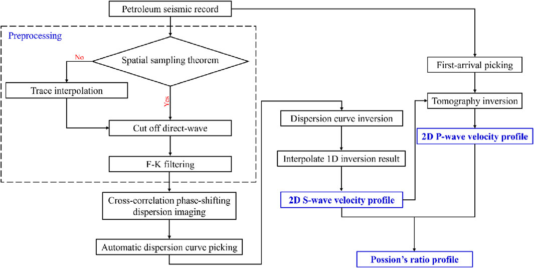
Figure 1. Flowchart of surface waves analysis method and surfaces wave and first-arrival joint velocity modeling.

2.1 Petroleum surface waves data analysis and preprocessing

As the energy of surface waves is primarily concentrated within approximately one wavelength depth near the earth’s surface and cannot directly carry deep subsurface information, in petroleum exploration, field instrument acquisition, observational system design, and subsequent processing and interpretation primarily focus on seismic reflection waves. In contrast, surface waves are considered interference and are suppressed. The information of surface waves acquisition in the field is often compromised, with incomplete recorded data and significant alias problem, making it challenging to be directly utilized. Therefore, necessary preprocessing is required for the recorded seismic surface waves, such as applying F-K filtering to eliminate the influence of other noise. In comparison to engineering exploration, petroleum exploration operates on a larger scale, introducing inevitable challenges like uneven topography and obstruction by buildings during seismic data acquisition. In such situations, field personnel may increase the spacing between receivers to overcome these obstacles. However, this results in the generation of significant spatial aliasing in surface waves dispersion imaging. Spatial aliasing diminishes the focusing capability of surface waves energy and can lead to misinterpretation during dispersion curves picking. Consequently, for these challenges, interpolation within traces becomes necessary (Li, 1987). Wang et al. (2019) proposed a method based on optimal wavelet bases for seismic surface waves interpolation, effectively eliminating spatial aliasing arising from excessive trace spacing. This section provides only a brief introduction to the method and detailed derivations can be found in the relevant literature.

As shown in Figure 2, using the first-level two-dimensional wavelet transform, the high-resolution seismic record c0 is decomposed into four low-resolution sub-bands: the low-frequency component a1 and the high-frequency components h1, v1, and d1 in the horizontal, vertical, and diagonal directions, respectively. Subsequently, a second-level two-dimensional wavelet transform is applied to the low-frequency component a1, resulting in four new sub-bands: a2, h2, v2, and d2. The wavelet inverse transform involves iteratively merging these four sub-bands through mathematical methods to reconstruct a large sub-band, ultimately obtaining the original record c0.

Figure 2

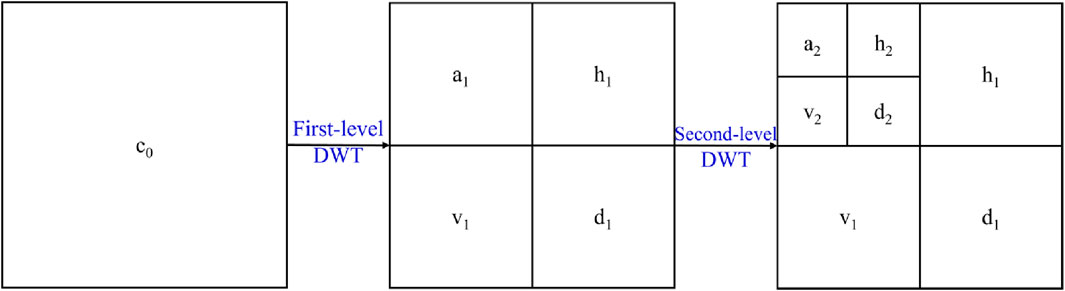
Figure 2. Sketch map of wavelet transform.

By analogy to the process of the wavelet inverse transform, the original seismic data can be viewed as the low-frequency component in the second-level wavelet transform sub-bands. Assuming that the original record shares the same structural information as the high-resolution seismic record, filtering and frequency modulation are applied to the original record to estimate the high-frequency details of the approximately high-resolution seismic record. Finally, interpolation is completed through a two-dimensional wavelet inverse transform. This approach of estimating high-frequency details of the high-resolution seismic record avoids the drawback of zeroing out high-frequency components in traditional interpolation methods, preventing information loss and compensating to some extent for high-frequency details. As surface waves have a relatively large phase velocity, direct interpolation of them may result in poor performance. Therefore, linear moveout correction can be applied to the phase velocity of surface waves before the interpolation process. After interpolation, a reverse moveout correction is then performed to restore the phase velocity of surface waves.

The interpolation results are shown in Figure 3. The original record, as depicted in Figure 3A, consists of 40 traces sampled every 2 ms, with a recording duration of 8 s. After interpolation, a total of 160 seismic traces are obtained, as depicted in Figure 3B. Dispersion imaging of the seismic data before and after interpolation is presented in Figure 3C,D. A comparison reveals that interpolation eliminates spatial aliasing and false high-order modes present in the original dispersion imaging, providing high signal-to-noise ratio dispersion imaging for subsequent dispersion curve picking.

Figure 3

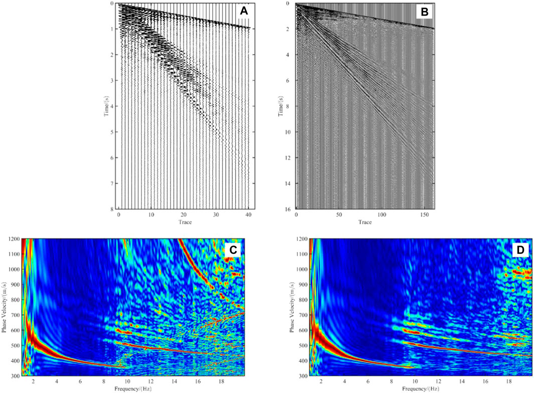
Figure 3. Comparison of seismic data and dispersion spectra before and after trace interpolation. (A) Seismic data before trace interpolation; (B) Seismic data after trace interpolation; (C) Dispersion spectra before trace interpolation; (D) Dispersion spectra after trace interpolation.

2.2 Dispersion imaging and dispersion curves picking

MASW (Multichannel Analysis of Surface Waves) technology identifies different frequency components of surface waves through the coherence of multi-channel records, providing high signal-to-noise ratio in surface waves dispersion imaging and enabling accurate picking of dispersion curves in subsequent steps. Over the course of more than 30 years of development, MASW has evolved various dispersion imaging methods, such as F-K transformation, τ-p transformation, phase-shift method, high-resolution linear Radon transformation, cross-correlation phase-shift method, and others (Gabriels et al., 1987; McMechan and Yedlin, 1981; Park et al., 1998; Luo et al., 2008; Liu et al., 2015; Wu et al., 2017). We utilize the cross-correlation phase-shift method (CCPS) proposed by Wu et al. (2017). Compared to conventional phase-shift methods, the cross-correlation phase-shift method exhibits stronger noise resistance, resulting in higher signal-to-noise ratio in the obtained dispersion imaging, as shown in Figure 4B. It is important to note that in petroleum exploration with long receiver arrays, near-field effects of surface waves (where surface waves have not yet developed into cylindrical waves near the receiver positions) need not be considered when applying surface wave analysis methods. However, the influence of far-field effects must be emphasized. If the receiver array distance is too long, surface wave energy sharply decreases. Dispersion imaging of seismic data in this part results in low signal-to-noise ratio, leading to misinterpretation in subsequent dispersion curves picking (Jiang et al., 2018). Additionally, dispersion imaging for thousands of receiver data simultaneously poses challenges to the computer’s processing power and memory. Therefore, it is essential to judiciously choose receiver positions and the number of receiver traces for dispersion imaging.

Figure 4

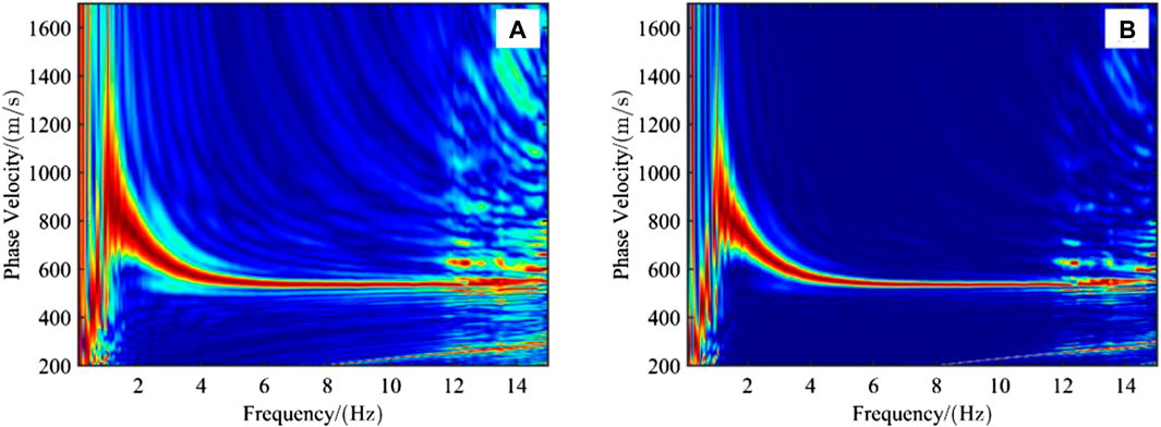
Figure 4. Comparison of phase-shifting method and cross-correlation phase-shifting method. (A) Phase-shifting method; (B) Cross-correlation phase-shifting method.

One of the distinctive features of petroleum exploration, different from natural seismology and engineering surveys, is the large volume of data. In a typical exploration area, there are often tens of thousands or even hundreds of thousands of shot points, with each shot point having thousands of receiver traces. Extracting dispersion curves using traditional manual identification and picking methods is inefficient and cannot guarantee accuracy. This limitation has been one of the reasons hindering the development of surface wave methods to the field of petroleum exploration. To address this problem, Wang et al. (2021) proposed a density-based DBSCAN (Density-Based Spatial Clustering of Applications with Noise) algorithm, which can identify and automatically pick dispersion curves of multi-mode surface waves based on density.

The automatic picking of multi-mode dispersion curves is a complex process that involves separating the dispersion energy from noise, identifying and classifying the dispersion energy of different modes. The process is shown in Figure 5. Initially, a three-dimensional Gaussian mixture model clustering (GMM clustering) method is employed to separate dispersion energy from background noise points. Subsequently, the DBSCAN algorithm is used to distinguish different dispersion energy modes. Finally, within different mode regions, Kalman filtering is applied to the dispersion energy to eliminate noise interference. The process involves searching for the maximum value at each frequency, resulting in the extraction of multi-mode dispersion curves of surface waves. The entire picking process, once parameters are initialized, does not require manual intervention and effectively enhances the accuracy and efficiency of surface wave data processing.

Figure 5

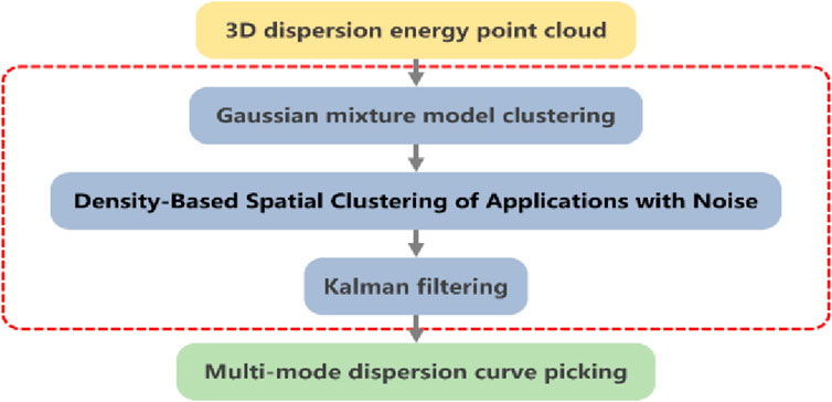
Figure 5. Automatic picking process of multi-mode dispersion curve.

2.3 Surface wave inversion and near surface velocity modeling

2.3.1 Inversion of dispersion curves for the simultaneous determination of velocity and thickness

The inversion of surface waves dispersion curves is an important section in surface waves analysis and a typical inverse problem in geophysics. Current main strategies for surface waves dispersion curves inversion can be categorized into linearized iterative inversion and global optimization inversion. Linearized iterative inversion typically focuses on inverting shear wave velocities of subsurface layers, while global optimization inversion aims to simultaneously invert both shear wave velocities and layer thicknesses. Considering the characteristics of petroleum exploration data, global optimization algorithms demand higher computational power, so may not be suitable for large-scale practical applications. Wu et al. (2017) innovatively drew inspiration from global optimization inversion, proposing a strategy that simultaneously regularizes linear inversion for both layer velocities and thicknesses. This approach effectively reduces dependency on initial models, enhancing the success rate of the inversion process.

In the context of the discussed surface wave dispersion curves inversion problem, the inversion objective function we have chosen can be specifically expressed as:

$\mathrm{\Phi }\left(\mathit{m}\right)={‖\mathit{W}\left[\mathit{d}-\mathit{f}\left(\mathit{m}\right)\right]‖}_2^2+\lambda {‖\mathit{L}\left(\mathit{m}-{\mathit{m}}_0\right)‖}_2^2(1)$

Here, ${‖\cdot ‖}_2^2$ denotes the square of the L-2 norm; d is the observed data vector, i.e., the surface waves dispersion curve data; f(m) is the theoretical predicted value vector, i.e., the dispersion curves data obtained through forward modeling; m0 is the initial model vector, including compressional wave velocity, density, and layer thicknesses; W is a diagonal matrix with elements composed of the standard deviation of the observed data; L is the roughness matrix; $\lambda$ is the regularization parameter used to balance the data fitting and model regularization terms.

Due to the simultaneous inversion of velocity and thickness, which introduces two physically distinct quantities with different dimensions, we learn from the experience of electromagnetic inversion and take the logarithm of both the inversion model parameters and observed data of Eq. 1 before solving:

$\begin{array}{l}\mathit{m}=\left[\ln \mathit{\beta },\ln \mathit{h}\right]=\left[\ln {\beta }_1,\ln {\beta }_2,\cdots ,\ln {\beta }_{\mathrm{M}},\ln h_1,\ln h_2,\cdots ,\ln h_{\mathrm{M}-1}\right]\\ \mathit{d}=\ln \mathit{c}=\left[\ln c_1,\ln c_2,\cdots ,\ln c_{\mathrm{N}}\right]\end{array}(2)$

Here, M represents the number of layers, $\mathit{\beta }=\left[{\beta }_1,{\beta }_2,\cdots ,{\beta }_{\mathrm{M}}\right]$ is the vector of layer shear wave velocities, $\mathit{h}=\left[h_1,h_2,\cdots ,h_{\mathrm{M}-1}\right]$ is the vector of thicknesses of each layer in the upper half-space, and $\mathit{c}=\left[c_1,c_2,\cdots ,c_{\mathrm{N}}\right]$ is the observed data consisting of N extracted surface wave dispersion curves. When the inversion process concludes when the modification of model parameters in consecutive iterations is less than the predefined threshold, indicating that the optimal model has been found.

In the multi-channel surface wave analysis method, Park et al. (1999) suggested that inverting dispersion curves using the MASW method would result in an averaging effect, yielding a one-dimensional shear wave velocity structure beneath the midpoint of the receiver array. Therefore, influenced by this concept, the processing is performed on multi-shot records, and all obtained one-dimensional inversion results are subjected to distance-reversed weighted interpolation to obtain a two-dimensional shear wave velocity profile along the entire receiver array.

2.3.2 Joint modeling of surface waves and first arrival

Based on the propagation mechanism of seismic waves near the earth’s surface (Wang, et al., 2022), both surface waves and first arrivals carry a significant amount of near-surface information. While first arrival tomography has developed over the years and is a mature technology with objective inversion results, capable of obtaining high-precision near-surface P-wave velocity models, it still has inherent limitations such as the inability to accurately identify velocity inversion interfaces and low-velocity zones, as shown in Figure 6. Additionally, it is challenging to acquire the shear wave velocity model (Liu et al., 2009). On the other hand, surface wave inversion methods not only compensate for the shortcomings of first arrival tomography in obtaining shear wave velocity models but also provide a way to address the limitations of first arrivals in the presence of a “Shadow Zone” by utilizing S-wave velocity information.

Figure 6

Figure 6. First-arrival travel time tomography inversion with low-velocity interlayer model. (A) Model with low-velocity interlayer; (B) Forward modeling of first-arrival travel time; (C) P-wave velocity in tomography inversion.

Wang et al. (2022) proposed a near-surface site characterization method based on Joint Iterative Analysis of First Arrival and Surface Waves (JIAFS). This method combines the advantages of First Arrival Travel Time (FATT) tomography and Multichannel Analysis of Surface Waves (MASW). Initially, the shear wave velocity (VS) model obtained from MASW is converted into a reference compressional wave velocity (VP) model based on the initial Poisson’s ratio. This model is then used to constrain the progress of FATT, helping overcome the inherent limitations of FATT in accurately identifying velocity inversion interfaces and low-velocity zones. Subsequently, the VP and VS models obtained from constrained FATT and MASW are used to update the Poisson’s ratio model. Moreover, these VP and Vs. models can serve as initial models for the next iteration of analysis. Through this iterative process, the two inversion methods can fully leverage their respective advantages.

3 Real case study

3.1 Circumstances of the site LH

The earth surface is extensively covered by the unconsolidated weathered strata in the northwest of China. This type of near surface circumstances poses challenges in seismic data processing, particularly for the static correction and seismic imaging as the accurate near-surface velocity model is fundamental for both procedures.

The LH site is located on the northwestern fringe of Qaidam Basin. According to the field geological surveys, the area is characterized by acute topographic undulation and complicated subsurface structures. In addition, due to the long-term weathering and denudation, older strata expose leading to higher shallow velocity in some sections. As the well-log data shown in Figure 7C, this well is located at an altitude of 1750 m, the P-wave velocities vary dramatically between 2000 m/s and 5,000 m/s, especially in the shallow strata which reach up to about 4,500 m/s.

Figure 7

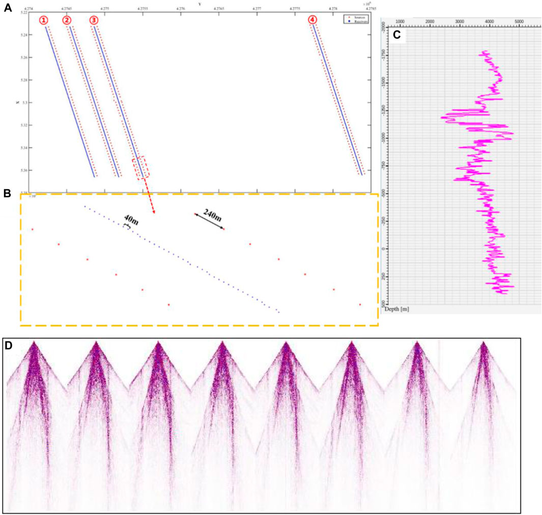
Figure 7. Geometry, logging data and seismic data. (A) Relative position of measuring line; (B) Geometry information; (C) Logging data; (D) Raw seismic data.

The seismic layout is shown in Figure 7A, which consist of four geophone receiver lines (blue dots) and seven explosive source lines (red dots). The data was extracted from a real 3D seismic survey for the method validation and denoted by ①, ②, ③, and ④ from left to right. Figure 7B is the enlarged view of red rectangular area in Figure 7A. It indicates that the inter-spacing of the receiver-points is 40 m and the inter-spacing of the source-points is 240 m. The recording time is 6 seconds and the sampling interval is 4 milliseconds. Eight typical shot records are shown in Figure 7D, from which we can see the well-developed first arrivals and surface waves (even higher modes).

3.2 Surface-wave processing of field data

3.2.1 Preprocessing

In order to obtain the reliable dispersion characteristics of surface waves, it is essential to preprocess the surface-wave data, otherwise the noises and the spatial aliasing would have adverse effects on the subsequent mode identification and picking in dispersion spectra. Figures 8A,C show one typical shot record and its original dispersion spectrum, respectively. Serious spatial aliasing occurs between 8 Hz and 20 Hz, as indicated in the red rectangular box. A similar situation happens between 16 Hz and 20 Hz due to the spatial aliasing of the first arrival of the body wave (Cheng et al., 2023), as shown in the yellow box. Hence, we cut off the first arrivals and conduct trace interpolation to resolve the problems.

Figure 8

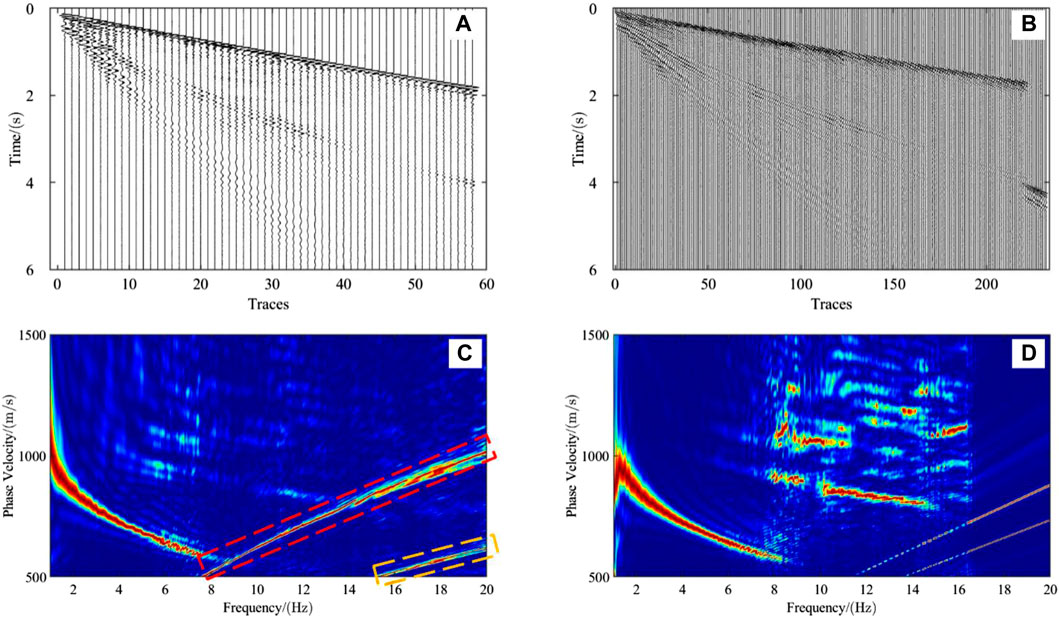
Figure 8. Comparison of seismic records and dispersion spectra before and after preprocessing. (A) Seismic records before channel interpolation; (B) Seismic records after channel interpolation; (C) Dispersion spectra before preprocessing; (D) Dispersion spectra after preprocessing.

Figure 8B shows the record after trace interpolation by the two-level wavelet inverse transformation, the channel number of which quadruples and the receiver spacing becomes a quarter of the initial value. The surface waves have been retained completely. Next, the first arrivals are removed and the F-K filtering are used to attenuate the noises. Finally, the surface-wave dispersion spectrum is acquired as shown in Figure 8D. Because the energy of spatial aliasing is strong, it has suppressed the energy of surface waves (Figure 8C). In Figure 8D, the spatial aliasing is removed and thus the higher-mode surface waves also appear apparently, which illustrates the validity of our interpolation method. Overall the preprocessing is applicable and effective in field data processing.

3.2.2 CCPS method and the dispersion-curve auto-picking by DBSCAN

The left 50 traces of the 30th shot and the right 50 traces of the 64th shot were selected on line ③ and dispersion imaging was performed using the CCPS method. As can be seen from Figure 9A, the surface wave in the 30th shot are very developed, with both fundamental and high-order modes. The events of the surface waves show a continuous, clearly recognizable “broom” shape. The surface wave energy on the right side of the 64th shot is relatively weakened, but higher-order modes can still be seen in the record. Overall, the reflected waves of these two sets of records are very weak and the surface wave development is uneven, which reflects the complexity of the subsurface structure and surface morphology. Figures 9C,D show the dispersion imaging of the above two gathers. Compared with the higher-order mode, the imaging quality of the fundamental-order mode is higher, and the resolution and continuity are better. However, the resolution of dispersive energy clusters is not good when frequencies less than 1 Hz, which is a common problem in the application of dispersive imaging to field data.

Figure 9

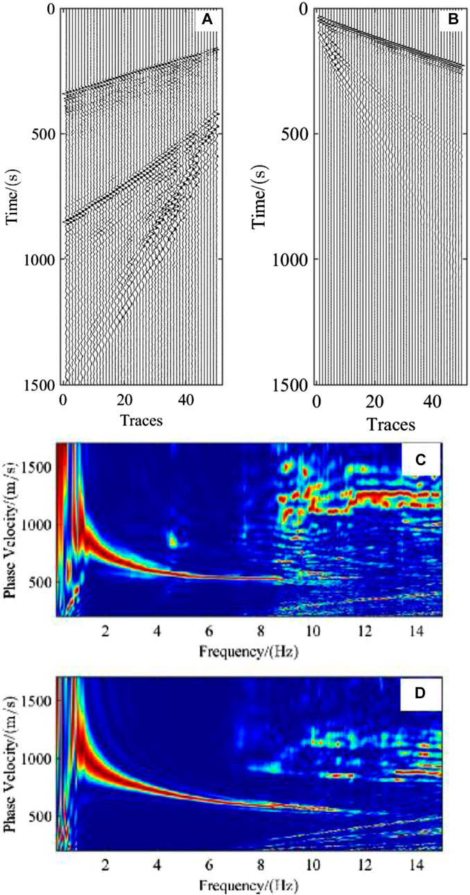
Figure 9. Partial gather of the 30th and 64th shots of Line 3. (A) Record of 50 tracks on the left side of the 30th shot; (B) Record of 50 tracks on the right side of the 64th shot; (C) Dispersion imaging of (A); (D) Dispersion imaging of (B).

In order to demonstrate the stability and accuracy of the DBSCAN automatic pickup algorithm in the face of multi-order modes, the first 50 traces of the 70th shot of line ② are selected for demonstration. As shown in Figure 10A, there are fundamental, higher first and higher second order dispersion energies in the frequency-phase velocity spectrum, but there are also strong noises at high frequencies.

Figure 10

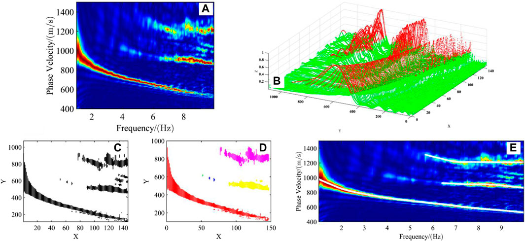
Figure 10. The automatic picking process of the dispersion curve of the 70th shot seismic record. (A) Dispersion imaging; (B) Energy threshold 3D map; (C) GMM clustering result; (D) DBSCAN clustering result; (E) Dispersion curve picking result.

Figure 10B shows a 3D comparison of energy thresholds for 70th shot frequency dispersion imaging, where the red region represents dispersive energy and the green region represents background noise. Applying the 3D GMM clustering algorithm to Figure 10B in the separation, we can obtain the dispersive energy and noise shown in Figure 10C. The dispersive energy is then subjected to DBSCAN clustering to identify and separate the different surface wave modes. The separation results are shown in Figure 10D, and it can be seen that the energy of the fundamental order, the first higher order, and the second higher order of the surface wave are accurately separated. In order to eliminate local outlier interference, Kalman filtering is applied to the regions with strong energy. Finally a reasonable energy maximum is picked up to obtain the dispersion curve, as shown by the white dot connection in Figure 10E. The same method was used to pick up the energy of the fundamental order of the 100th shot, and the results were also more accurate. The test of the DBSCAN automatic dispersion curve picking algorithm with this set of data found that each dispersion curve only takes about 0.42s. Compared with the manual picking, it greatly improves the efficiency.

3.3 Inversion of shear wave velocity and formation thickness using surface wave

In this section, the simultaneous inversion algorithm for velocity and thickness is used to invert the dispersion curve. The algorithm utilities two distinct physical parameters, velocity of shear wave and formation thickness, and exhibits reduced dependence on the initial model compared to other linear Jacobi iterative inversion algorithms. During the inversion process, an empirical approach is employed to set the initial model as 11 layers with each layer having a thickness of 10 m, while the 11th layer is half space. Figures 11A,B show the inversion results of two sets of dispersion curves in the survey line ④, whose geodetic coordinates X are 529,250 and 532,140, respectively. The left subgraph is the comparison between the actual picked dispersion curve points (green) and the dispersion curve points (red) obtained after the forward modeling of the final inversion model, and the right subgraph is the final 1-dimensional inversion results. By comparison, it is found that the dispersion curve obtained by inversion can match the actual dispersion curve well. The variation of 1-D inversion results in shallow layer is drastic, which accords with the geological characteristics of the working area.

Figure 11

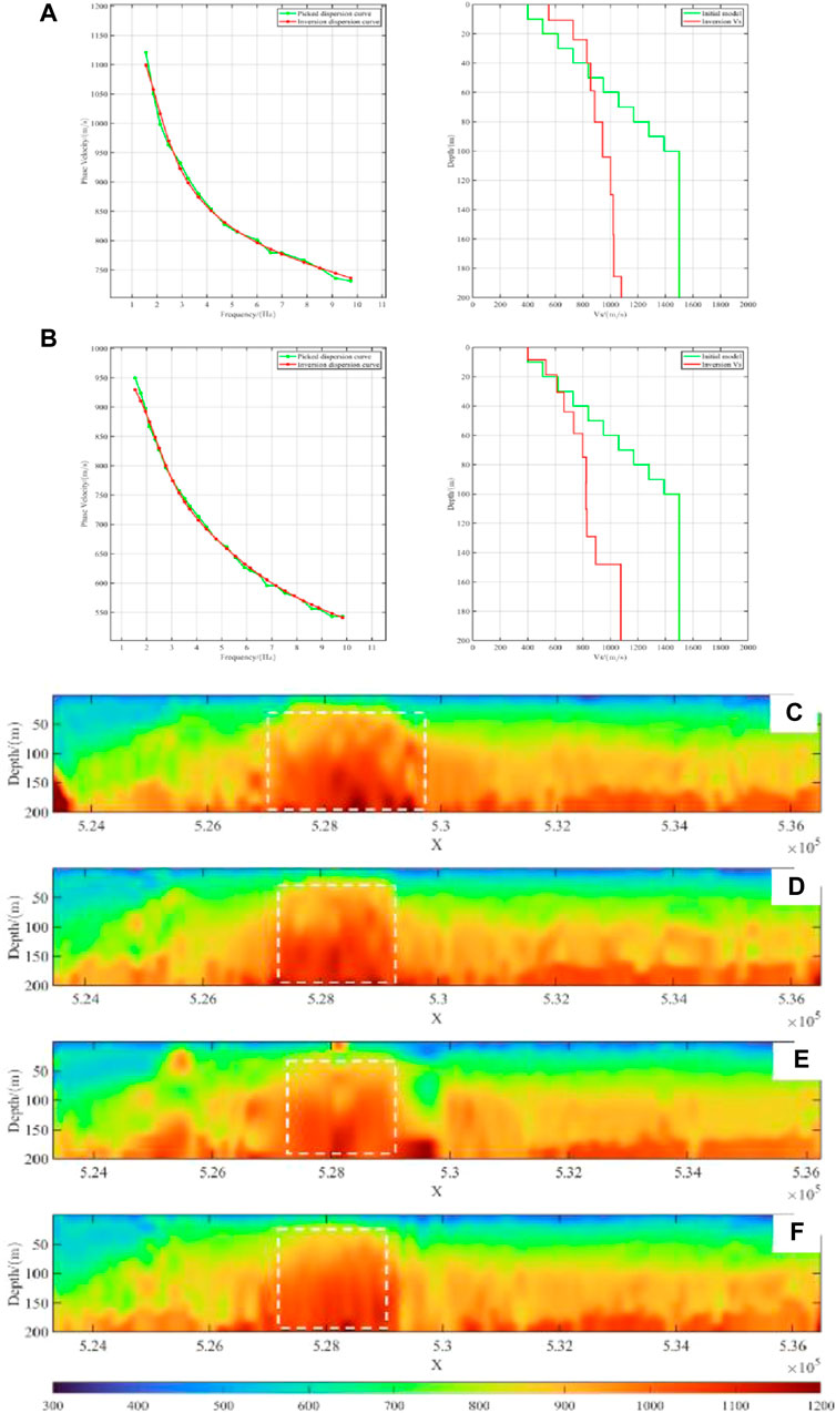
Figure 11. Results obtained from simultaneous inversion of velocity and thickness. (A) 1-Dimensional Inversion Results at Geodetic Coordinate X=529,250 of line 4; (B) 1-Dimensional Inversion Results at Geodetic Coordinate X=532,140 of line 4; (C) 2D inversion results of line 1; (D) 2D inversion results of line 2; (E) 2D inversion results of line 3; (F) 2D inversion results of line 4.

The inverted S-wave velocities in different geodetic coordinates for each survey line are interpolated with distance inverse weighting, and four 2D S-wave velocity profiles can be obtained (from Figure 11C to Figure 11F). By comparing and combining local micro-logging information, the S-wave velocity can be roughly divided into four zones. The first zone is a weathered zone with a depth range of approximately 1–20 m and S-wave velocities of 350–400 m/s, with the potential for deeper stratigraphic outcrops in this depth range. The second zone is the low-velocity zone, the depth ranges from 21 to 80 m, and the S-wave velocity is 600–800 m/s. High-velocity anomalies (shown in the white dashed box) begin to appear in this layer, and the geological interpretation is that the stratigraphy here have been uplifted because of the strong stratigraphic opposing extrusion within the range of X=528,000 ± 1,000, which resulted in the emergence of anticlinal structure. Because of the strong weathering, the low-velocity zone, which should be at the surface location, was weathered and eroded into a weathering zone, but the buffer zone and the high-velocity zone underneath were still preserved. The third zone is a buffer zone with a depth range of about 81–160 m and an S-wave velocity of 900–1,000 m/s. The fourth is a high-velocity zone, with depths below 160 m and S-wave velocities reaching over 1100 m/s.

3.4 Near-surface modeling by surface wave and first-arrival joint inversion

Before first-arrival tomography, it is necessary to pick up the first-arrival of the actual seismic data. Based on the characteristic that the amplitude of the first-arrival signal is larger than that of the noise signal, a modified energy-ratio method is used here (Zuo et al., 2004). The method normalizes the energy in the region near the first-arrival signal and then picks up the first-arrival travel time according to the signal energy ratio and amplitude threshold criteria. The pickup process and effect are shown in Figure 12, the red solid line is the first-arrival picked up, and the blue and green dashed lines are the delineated energy identification range. Overall the energy ratio method is effective and the pickup result is accurate.

Figure 12

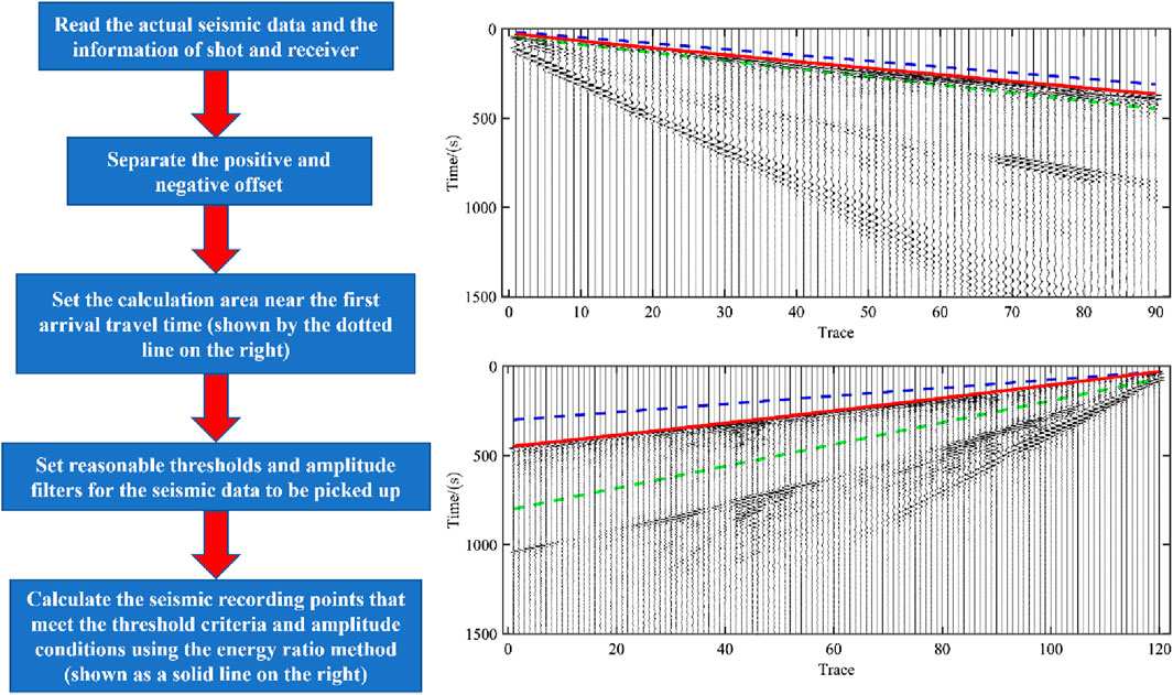
Figure 12. Display of the first-arrival and flowchart of first-arrival picking using the energy ratio method.

Due to the complex geological conditions in the LH site, it is impossible to carry out the first-arrival tomography technique alone. As shown in Figure 13, taking the first-arrival tomography of survey line ② as an example, the first-arrival tomography demonstrates a more objective lateral resolution. However, the high-velocity uplift region affects a portion of the ray tracing, resulting in missing information and making the inversion of the right part of the profile poor. Compared to the surface wave inversion results (shown in Figure 11D), the vertical resolution of the first-arrival tomography is poor. It is impossible to distinguish the weathered layer from the low-velocity zone in the shallow layers, which is an inherent defect of the first-arrival tomography. In addition, the details of the intrusion of the high-velocity body are also not as fine as they could be. Therefore, the joint near-surface modeling technique of surface waves and first-arrival can be applied to the actual data in this area to improve the inversion accuracy of first-arrival tomography as well as to improve the detail portrayal.

Figure 13

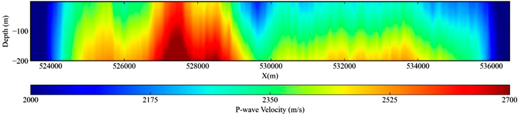
Figure 13. First-arrival tomography inversion profile of line 2.

As shown in Figures 14A,B P-wave velocity profiles with a depth of 500 m were obtained for survey line ③ using FATT and JIAFS, respectively. The inversion profile shows that the subsurface transverse velocity of the line is very strong, and the low-velocity stratum is thin. The high-velocity strata are developed and very thick, and at some depths the high-velocity strata have intruded into the shallow low-velocity strata. The stratigraphy is basically horizontal except in the range of X=528,000 ± 1,000, where the stratigraphy shows anticlinal structure due to extrusion. The velocity increases from shallow to deep, which can coincide with the conclusion of the geological interpretation obtained by MASW. The comparison reveals that when the surface wave inversion results are used to constrain the stratigraphic inversion, it improves the detail of the P-wave velocity profiles, especially in the shallow, low-velocity regions with little ray coverage, as shown by the white dashed ellipse in Figure 14B. In order to further illustrate the effect of JIAFS, the inversion results of JIAFS and FATT are selected in the same shallow area for comparison. As shown in Figures 14C,D, the joint inversion “pulls up” the trend of the inversion velocity interface, which effectively improves the correspondence between the inversion results and the micro-logging.

Figure 14

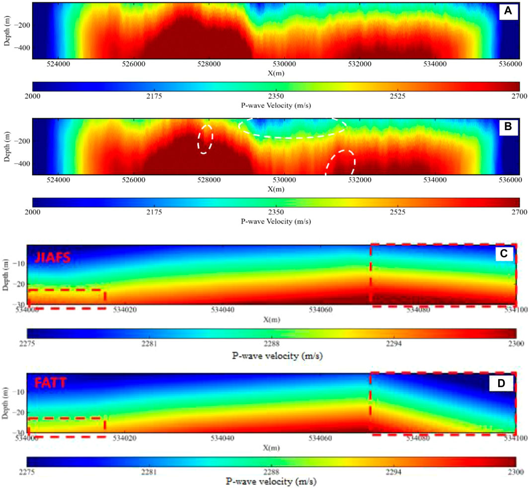
Figure 14. First-arrival tomography inversion profile and surface wave and first break joint inversion profile of Line 3. (A) FATT; (B) JIAFS; (C) shallow area of (A); (D) shallow area of (B).

JIAFS is capable of obtaining Poisson’s ratio profiles using wave velocity information from MASW and FATT, in addition to P-wave velocity profiles with high accuracy. The Poisson’s ratio profiles of the four survey lines obtained by JIAFS are shown in Figure 15. As can be seen in Figure 15, the shallow Poisson’s ratio is very high, indicating extremely severe surface weathering in this area. The Poisson’s ratio decreases with depth, indicating that the stratigraphic rocks are getting denser with depth. There is a region of very low Poisson’s ratio in the range X = 528,000 ± 1,000, which has been explained earlier when analyzing the velocity profiles and will not be repeated here.

Figure 15

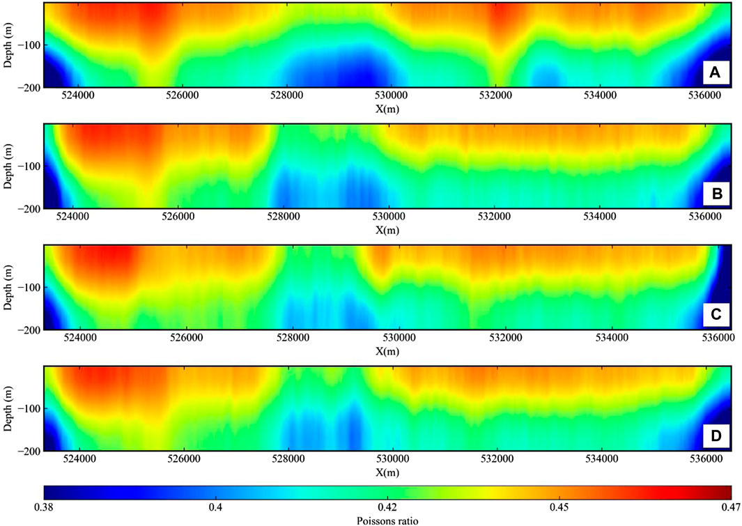
Figure 15. Poisson’s ratio profile obtained by JIAFS. (A) Line 1; (B) Line 2; (C) Line 3; (D) Line 4.

4 Discussions and conclusions

With the development of oil and gas exploration, accurate modeling of near surface velocity has become a prerequisite for determining the accuracy of some imaging techniques. Although near surface velocity modeling methods such as micro logging, refracted wave method, first-arrival tomography, and full waveform inversion have been developed, they all encounter some constraints. Micro logging has the problem of high cost and low efficiency. Refracted wave method relies on the quality of seismic data and the stability of underground refractive interfaces. Although first-arrival tomography can obtain objective and reliable P-wave velocity profiles, it is difficult to obtain S-wave velocity profiles. And high-velocity anticlines can affect the accuracy of ray tracing. Due to computational limitations, full waveform inversion is currently difficult to apply on a large scale in the petroleum exploration.

As a type of seismic wave grown near the surface, surface waves carry a large amount of near surface S-wave velocity information. Therefore, surface wave analysis methods in the engineering exploration can be used to guide the application of surface waves in petroleum seismic data. Obtaining near-surface S-wave velocity profiles with good vertical resolution through surface waves data processing and dispersion curve inversion. At the same time, the use of Poisson’s ratio can link surface wave analysis methods with first-arrival tomography, which can take advantage of each other’s strengths and improve the accuracy of near surface velocity modeling.

This paper successfully applied surface wave analysis methods to extract the near-surface shear wave velocity profile from petroleum seismic data in the LH site of Qinghai, China. The underground depth range of 0–200 m was divided into four geological zones, and the presence of subsurface anticlinal structures was identified. Subsequently, a joint modeling approach combining surface waves and first arrivals was employed to obtain the compressional wave velocity profile and Poisson’s ratio profile at a depth of 500 m. This approach addressed the limitations of using first arrival tomography alone and validated the geological interpretation obtained from surface wave inversion.

The research findings indicate that surface wave analysis methods can be effectively applied to petroleum seismic data, and their combination with first arrival tomography provides a more objective and accurate characterization of near-surface velocity models. However, it is essential to emphasize the importance of surface wave data processing in petroleum exploration. Preprocessing and high signal-to-noise ratio dispersion imaging are crucial for handling low-quality data. Otherwise, spatial aliasing or noise generated during the process may suppress the energy of surface waves at various orders, leading to misinterpretations during subsequent dispersion curve picking.

In summary, this research expands the application scope of surface wave analysis methods, demonstrating their utility in petroleum exploration. It transforms surface wave data in petroleum exploration into valuable information, providing theoretical and technical support for practical data processing and inversion in future petroleum exploration endeavors.

Data availability statement

The datasets presented in this article are not readily available because Data is confidential and cannot be copied or transmitted. Requests to access the datasets should be directed to YT, 632856428@qq.com.

Author contributions

XX: Methodology, Writing–original draft, Writing–review and editing. YT: Writing–review and editing. DW: Methodology, Software, Writing–original draft. JX: Investigation, Writing–review and editing. ZW: Writing–original draft. TZ: Writing–review and editing.

Funding

The author(s) declare financial support was received for the research, authorship, and/or publication of this article. This work is supported by the Scientific Research and Technology Development Project of PetroChina Co., LTD, under Grant No. 2022KT1503.

Conflict of interest

Authors XX, YT, DW, JX, and TZ were employed by PetroChina.

Author ZW was employed by Huabei Oilfield Company.

Publisher’s note

All claims expressed in this article are solely those of the authors and do not necessarily represent those of their affiliated organizations, or those of the publisher, the editors and the reviewers. Any product that may be evaluated in this article, or claim that may be made by its manufacturer, is not guaranteed or endorsed by the publisher.

Supplementary material

The Supplementary Material for this article can be found online at: https://www.frontiersin.org/articles/10.3389/feart.2024.1379668/full#supplementary-material

References

Askari, R., Ferguson, R. J., Isaac, J. H., and Hejazi, S. H. (2015). Estimation of S-wave static corrections using CMP cross-correlation of surface waves. J. Appl. Geophys. 121, 42–53. doi:10.1016/j.jappgeo.2015.07.004

CrossRef Full Text | Google Scholar

Ballard, R. F. (1964). Determination of soil shear moduli at depths by in-situ vibratory techniques. Waterways Experiment Station. Misc. Pap., 4–691. doi:10.1016/0022-4898(70)90136-9

CrossRef Full Text | Google Scholar

Boiero, D., Wiarda, E., and Vermeer, P. (2013). Surface- and guided-wave inversion for near-surface modeling in land and shallow marine seismic data. Lead. Edge 32 (6), 638–646. doi:10.1190/TLE32060638.1

CrossRef Full Text | Google Scholar

Boué, A., Courbis, R., Chmiel, M., Arndr, M., and Gradon, C. (2019). Vs imaging from ambient noise Rayleigh wave tomography for oil exploration. Nevada, United States: SEG Technical Program Expanded Abstracts, 5382–5385. doi:10.1190/segam2019-w21-01.1

CrossRef Full Text | Google Scholar

Cheng, F., Xia, J., and Xi, C. (2023). Artifacts in high-frequency passive surface wave dispersion imaging: toward the linear receiver array. Surv. Geophys. 44, 1009–1039. doi:10.1007/s10712-023-09772-1

CrossRef Full Text | Google Scholar

Ernst, F. E. (2007). “Long-wavelength statics estimation from guided waves,” in EAGE 69th conference and exhibition incorporating SPE EUROPEC, cp-27-00194. doi:10.3997/2214-4609.201401612

CrossRef Full Text | Google Scholar

Gabriels, P., Snieder, R., and Nolet, G. (1987). In situ measurements of shear-wave velocity in sediments with higher-mode Rayleigh waves. Geophys. Prospect. 35 (2), 187–196. doi:10.1111/j.1365-2478.1987.tb00812.x

CrossRef Full Text | Google Scholar

Ikeda, T., Tsuji, T., Takanashi, M., Kurosawa, I., Nakatsukasa, M., Kato, A., et al. (2017). Temporal variation of the shallow subsurface at the Aquistore CO2 storage site associated with environmental influences using a continuous and controlled seismic source. J. Geophys. Res. Solid Earth 122 (4), 2859–2872. doi:10.1002/2016JB013691

CrossRef Full Text | Google Scholar

Jiang, F. H., Li, P. M., Zhang, Y. M., Yan, Z. H., and Dong, L. Q. (2018). Frequency dispersion analysis of MASW in real seismic data. Oil Geophys. Prospect. (in Chin.) 53 (1), 17–24. doi:10.13810/j.cnki.issn.1000-7210.2018.01.003

CrossRef Full Text | Google Scholar

Jones, R. (1962). Surface wave technique for measuring the elastic properties and thickness of roads: theoretical development. Br. J. Appl. Phys. 13 (1), 21–29. doi:10.1088/0508-3443/13/1/306

CrossRef Full Text | Google Scholar

Kim, D., Banerdt, W. B., Ceylan, S., Giardini, D., Lekić, V., Lognonné, P., et al. (2022). Surface waves and crustal structure on Mars. Science 378 (6618), 417–421. doi:10.1126/science.abq7157

PubMed Abstract | CrossRef Full Text | Google Scholar

Krohn, C. E., and Routh, R. S. (2010). Exploiting surface consistency for ground-roll characterization and mitigation. Seg. Tech. Program Expand. Abstr. 1, 1892–1896. doi:10.1190/1.3513211

CrossRef Full Text | Google Scholar

Krohn, C. E., and Routh, R. S. (2017). Exploiting surface consistency for surface-wave characterization and mitigation — Part 1: theory and 2D examples. Geophysics 82 (1), V21–V37. doi:10.1190/geo2016-0019.1

CrossRef Full Text | Google Scholar

Laake, A., and Strobbia, C. (2012). Multi-measurement integration for near-surface geological characterization. Near Surf. Geophys. 10 (6), 591–600. doi:10.3997/1873-0604.2012008

CrossRef Full Text | Google Scholar

Li, Q. Z. (1987). Seismic signal interpolation and noise deletion (1). Chin. J. Geophys. (in Chinese) 30 (5), 514–531

Google Scholar

Li, X. Y., Chen, X. F., Yang, Z. T., Wang, B., and Yang, B. (2020). Application of high-order surface waves in shallow exploration: an example of the Suzhou river, Shanghai. Chinese Journal of Geophysics (in Chinese) 63 (1), 247–255. doi:10.6038/cjg2020N0202

CrossRef Full Text | Google Scholar

Liu, Q. H., Lu, L. Y., and Wang, K. M. (2015). Review on the active and passive surface wave exploration method for the near-surface structure. Progress in Geophysics (in Chinese) 30 (6), 2906–2922. doi:10.6038/pg20150660

CrossRef Full Text | Google Scholar

Liu, Y., Dong, L., Wang, Y., Zhu, J., and Ma, Z. (2009). Sensitivity kernels for seismic Fresnel volume tomography. Geophysics 74 (5), U35–U46. doi:10.1190/1.3169600

CrossRef Full Text | Google Scholar

Liu, Y. H., Enhedelihai, H., Zhang, Y. H., and Yang, P. (2021). Application of surface wave based full waveform inversion on detection of shallow-buried obstruction. Progress in Geophysics (in Chinese) 36 (4), 1702–1710. doi:10.6038/pg2021EE0320

CrossRef Full Text | Google Scholar

Luo, Y., Xia, J., Miller, R. D., Xu, Y., Liu, J., and Liu, Q. (2008). Rayleigh-wave dispersive energy imaging using a high-resolution linear Radon transform. Pure and Applied Geophysics 165, 903–922. doi:10.1007/s00024-008-0338-4

CrossRef Full Text | Google Scholar

Mabrouk, W. M., Saleh, A. A., Ghanem, K. G., and Sharafeldin, S. M. (2017). A comparative study of near-surface velocity model building derived by 3D travel time tomography and dispersion curves inversion techniques. Journal of Petroleum Science and Engineering 154, 126–138. doi:10.1016/j.petrol.2017.04.023

CrossRef Full Text | Google Scholar

McMechan, G. A., and Yedlin, M. J. (1981). Analysis of dispersive waves by wave field transformation. Geophysics 46 (6), 869–874. doi:10.1190/1.1441225

CrossRef Full Text | Google Scholar

Park, C. B., Miller, R. D., and Xia, J. (1998) “Imaging dispersion curves of surface waves on multi-channel record,” in SEG technical program expanded abstracts 1998. New Orleans: Society of Exploration Geophysicists, 1377–1380. doi:10.1190/1.1820161

CrossRef Full Text | Google Scholar

Park, C. B., Miller, R. D., and Xia, J. (1999). Multichannel analysis of surface waves. Geophysics 64 (3), 800–808. doi:10.1190/1.1444590

CrossRef Full Text | Google Scholar

Petrova, N. V., and Gabsatarova, I. P. (2020). Depth corrections to surface-wave magnitudes for intermediate and deep earthquakes in the regions of North Eurasia. Journal of Seismology 24 (1), 203–219. doi:10.1007/s10950-019-09900-8

CrossRef Full Text | Google Scholar

Rayleigh, L. (1885). On waves propagated along the plane surface of an elastic solid. Proceedings of the London Mathematical Society 17, 4–11. doi:10.1112/plms/s1-17.1.4

CrossRef Full Text | Google Scholar

Strobbia, C., Vermeer, P., Laake, A., Glushchenko, A., and Re, S. (2010). Surface waves: processing inversion and removal. First Break 28, 85–91. doi:10.3997/1365-2397.28.8.40748

CrossRef Full Text | Google Scholar

Sun, Z. W., Gu, Y. M., Xu, G., Zhao, J. Z., and Zhang, J. D. (2010). Reconstruction of the high-resolution near-surface velocity model and its application to the static correction under complex surface conditions. Progress in Geophysics (in Chinese) 25 (5), 1757–1762. doi:10.3724/SP.J.1231.2010.06586

CrossRef Full Text | Google Scholar

Wang, Z., Sun, C., and Wu, D. (2019). Seismic surface wave interpolation method based on optimistic wavelet basis. Geophysical and Geochemical Exploration 43 (1), 189–198. doi:10.11720/wtyht.2019.1216

CrossRef Full Text | Google Scholar

Wang, Z., Sun, C., and Wu, D. (2021). Automatic picking of multi-mode surface-wave dispersion curves based on machine learning clustering methods. Computers & Geosciences 153, 104809. doi:10.1016/j.cageo.2021.104809

CrossRef Full Text | Google Scholar

Wang, Z., Sun, C., and Wu, D. (2022). Near-surface site characterization based on joint iterative analysis of first-arrival and surface-wave data. Surveys in Geophysics 44 (2), 357–386. doi:10.1007/s10712-022-09747-8

CrossRef Full Text | Google Scholar

Wu, D., Sun, C., and Lin, M. (2017). Activeseismic surface wave dispersion imaging method based on cross-correlation and phase-shifting. Progress in Geophysics (in Chinese) 32 (4), 1693–1700. doi:10.6038/pg20170437

CrossRef Full Text | Google Scholar

Xia, J., Miller, R. D., and Park, C. B. (1999). Estimation of near-surface shear-wave velocity by inversion of Rayleigh waves. Geophysics 64 (3), 691–700. doi:10.1190/1.1444578

CrossRef Full Text | Google Scholar

Xia, J. H., Xu, Y. X., Luo, Y. H., Richard, D. M., Recep, C., and Chong, Z. (2012). Advantages of using Multichannel analysis of Love waves (MALW) to estimate near-surface shear-wave velocity. Survey in Geophysics 33 (5), 841–860. doi:10.1007/s10712-012-9174-2

CrossRef Full Text | Google Scholar

Zuo, G. P., Wang, Y. C., and Sui, R. L. (2004). An improved method for first arrival pickup using energy ratio. Geophysical Prospecting for Petroleum (in Chinese) 43 (4), 345–347. doi:10.3969/j.issn.1000-1441.2004.04.008

CrossRef Full Text | Google Scholar