
94% of researchers rate our articles as excellent or good
Learn more about the work of our research integrity team to safeguard the quality of each article we publish.
Find out more
ORIGINAL RESEARCH article
Front. Earth Sci. , 09 May 2024
Sec. Atmospheric Science
Volume 12 - 2024 | https://doi.org/10.3389/feart.2024.1379069
This article is part of the Research Topic Tropical Cyclone Modeling and Prediction: Advances in Model Development and Its Applications View all 13 articles
 Weiguo Wang1*Jongil Han2Junghoon Shin3Xiaomin Chen4Andrew Hazelton5,6Lin Zhu1Hyun-Sook Kim6Xu Li3Bin Liu3Qingfu Liu2John Steffen1Ruiyu Sun2Weizhong Zheng3Zhan Zhang2Fanglin Yang2
This document summarizes the physics schemes used in two configurations of the first version of the operational Hurricane Analysis and Forecast System (HAFSv1) at NOAA NCEP. The physics package in HAFSv1 is the same as that used in NCEP global forecast system (GFS) version 16 except for an additional microphysics scheme and modifications to sea surface roughness lengths, boundary layer scheme, and the entrainment rate in the deep convection scheme. Those modifications are specifically designed for improving the simulation of tropical cyclones (TCs). The two configurations of HAFSv1 mainly differ in the adopted microphysics schemes and TC-specific modifications in addition to model initialization. Experiments are made to highlight the impacts of TC-specific modifications and different microphysics schemes on HAFSv1 performance. Challenges and developmental plans of physics schemes for future versions of operational HAFS are discussed.
Based on NOAA’s unified forecast system (UFS) framework, Hurricane Analysis and Forecast System (HAFS) is a UFS application specialized in tropical cyclone (TC) research and forecasting, which has been under active development with collaborative efforts among multiple agencies as well as the broader research communities. The first operational implementation of HAFS (HAFSv1) at NCEP occurred in June 2023 as a planned replacement for operational Hurricane Weather Research and Forecasting (HWRF) model (Tallapragada, 2016) and the Hurricane Multi-scale Ocean-coupled Non-hydrostatic (HMON) model (Mehra et al., 2018; Wang et al., 2019). The newly-developed HAFS was highlighted in the 10th WMO international workshop for TCs held in December 2022 as one of the most important developments of TC dynamic modeling during the last 4 years because it has shown the capability to further improve dynamic model guidance for TC track and intensity (Zhang et al., 2023). Multiple configurations of HAFS have been used in real-time experiments since 2019 to improve model performance. Before 2021, all experiments, including a HAFS-based ensemble system (Zhang et al., 2021), were based on a fixed basin-scale domain with high resolution (3 km) and without a vortex initialization process (Dong et al., 2020; Hazelton et al., 2021; Chen et al., 2023). The moving nest capability and a combined vortex modification and data assimilation system was developed and added to HAFS in late 2021; these additions were tested in the 2022 real-time experiment (Hazelton et al., 2023a).
The operational HAFSv1 is configured as a convection-allowing high resolution atmosphere-ocean-wave coupled TC forecasting system with one storm-following moving nest, advanced vortex initialization, data assimilation, and physics suite that is specially calibrated for hurricane predictions taking into account multiscale interactions (Zhang et al., 2023). The atmospheric model dynamics is based on the fully compressible Finite-Volume Cubed-Sphere (FV3) dynamical core (Lin and Rood, 1996; Lin, 1997; Lin and Rood, 1997; Lin, 2004; Harris et al., 2020) with a Lagrangian vertical coordinate (Chen et al., 2013). The ocean model implemented in HAFS is HYbrid Coordinate Ocean Model (HYCOM) (Bleck, 2002; Bleck et al., 2002). HAFSv1 has two configurations (HFSA and HFSB) to maintain the current operational capability of dynamical model diversity, with the former replacing HWRF and the latter replacing HMON. Like the HWRF and HMON models, both HFSA and HFSB are configured with one movable and two-way interactive nested horizontal grid that follows the projected path of a storm. Both HFSA and HFSB use an Extended Schmidt Gnomonic (ESG) horizontal grid system (Purser et al., 2020), with spatial resolutions of 6 km in the parent domain and 2 km in the nested domain. In addition, both configurations use 81 vertical levels on a sigma-pressure hybrid system with a model top of 10 hPa and the lowest level approximately at 20 m above the surface. There are 23 levels below 1.5 km, with vertical grid spacing varying approximately from 20 m near the surface to 130 m near 1.5 km, to reasonably resolve physical processes in the planetary boundary layer (PBL). A major difference between HFSA and HFSB is in microphysics schemes they used. The single-moment GFDL (Geophysical Fluid Dynamics Laboratory) microphysics scheme (Lin et al., 1983; Lord et al., 1984; Krueger et al., 1995; Chen and Lin, 2013) is used in HFSA, while the double-moment Thompson microphysics scheme (Thompson and Eidhammer, 2014) is used in HFSB. Because the double-moment Thompson scheme is more computationally costly than the single-moment GFDL scheme, HFSB uses a slightly smaller parent domain and lower calling frequency of the radiation scheme than HFSA to guarantee the running time of HFSB forecast jobs fit within the operational time window. Other differences include adjustments in the PBL and convection schemes and the thresholds used in the vortex initialization process. Zhang et al. (2023) gives the details of HFSA and HFSB as well as the development history of HAFS.
In this paper, we will describe the physics schemes used in both HFSA and HFSB, with a focus on TC-specific modifications and microphysics schemes. Section 2 summarizes individual physics schemes. Section 3 describes HAFS experiments used to highlight the impacts of different microphysics schemes and TC-specific modifications on the performance of HAFSv1. Challenges and future developmental plans of HAFS physics schemes are discussed in Section 4. A summary is provided in Section 5.
In general, HAFSv1 uses the same physics schemes as in the NCEP Global Forecast System version 16 (GFSv16), except for a few TC-specific modifications for better TC intensity forecasts and different microphysics schemes for diversity of the configurations. Table 1 summarizes the physics schemes used in both configurations of operational HAFSv1. The main differences in physics schemes between HAFSv1 and the legacy HWRF and HMON are in the selection of surface layer, PBL, and microphysics schemes. HWRF and HMON use the GFDL surface layer scheme (Bender et al., 2007), GFS hybrid K-based Eddy-Diffusivity Mass-Flux (EDMF) PBL scheme with TC-specific modifications (Han et al., 2016; Wang et al., 2018), and the Ferrier-Aligo microphysics scheme (Ferrier et al., 2002; Aligo et al., 2018). In this section, the physics schemes and modifications in HAFSv1 are briefly described.
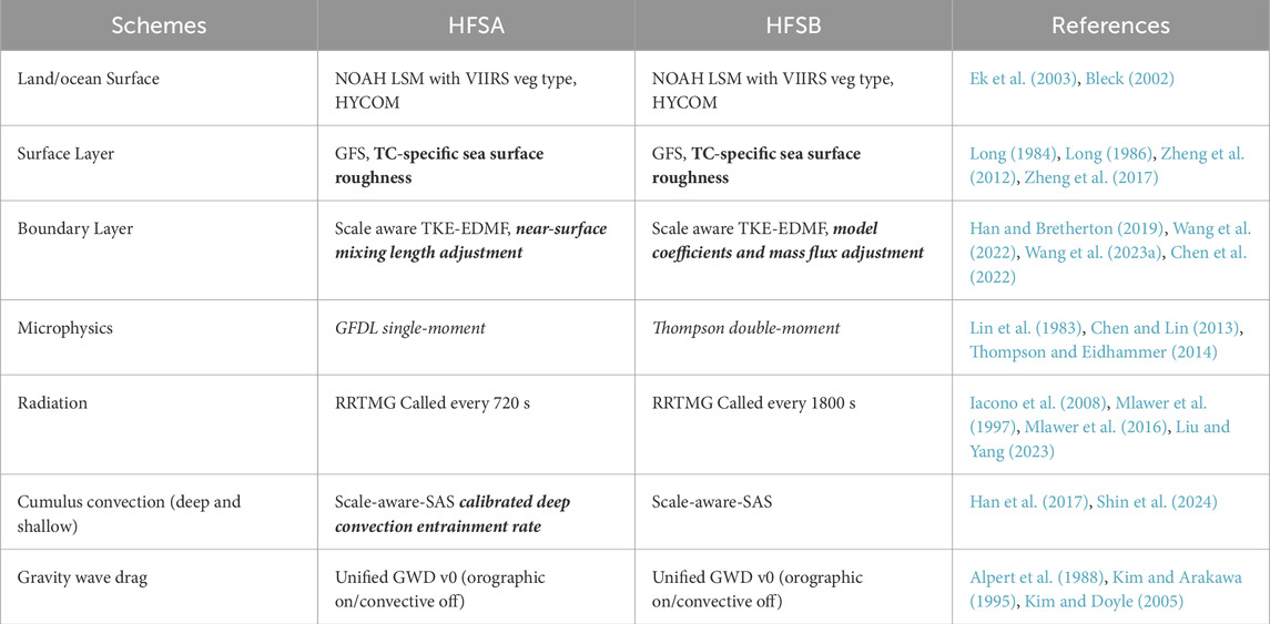
Table 1. Physics schemes used in HFSA and HFSB. (TC-specific modifications are marked in bold and differences between HFSA and HFSB are marked in italics).
The Noah land surface model (LSM) is used in HAFSv1 to characterize hydrological processes over land. The model is derived originally from the Oregon State University land surface model and has a long history of development. It provides surface sensible and latent heat fluxes, skin temperature, albedo, and other quantities to the atmospheric model. The Noah LSM includes a four-layer soil model, with the thickness of 0.1, 0.3, 0.6, and 1 m, respectively, from top to bottom. It solves the prognostic equations for soil temperature and moisture with the parameterized physical processes of surface energy and water budgets, including precipitation, surface runoff and infiltration, canopy evaporation and transpiration, soil evaporation, sublimation from snowpack, and more. The model uses a few look-up tables to prescribe soil, vegetation, and other general parameters in addition to key input datasets including land-use/vegetation type, soil texture, and slope. The NASA Visible Infrared Imaging Radiometer Suite (VIIRS) vegetation type is used in HAFSv1. Ek et al. (2003) gives a detailed description of the Noah model, its evolution, refinements, as well as key references of the schemes for various physical processes.
HYCOM solves three-dimensional hydrostatic primitive equations without tides at 1/12-degree resolution on the Arakawa C grid and 41 hybrid-z vertical coordinates (Bleck, 2002; Chassignet et al., 2003; Wallcraft et al., 2009). HYCOM in HAFSv1 uses the same solver and model grids as in the NCEP global Real-Time Ocean Forecast System (RTOFS), except it is a regional application (Kim et al., 2014; Kim et al., 2022). The regional domain covers the Atlantic, eastern Pacific, and central Pacific basins from 23.03oS to 47.0oN in latitude and from 182oE to 15.0oE in longitude. The lateral boundaries are closed with a buffer zone with 10 horizontal grid spacings, to relax the interior solutions to the climatology. The initial conditions (ICs) for each cycle are provided by subsets of daily nowcast and forecast products of the global RTOFS. The global nowcasts are analyses produced from a flow-dependent three-dimensional variational data assimilation system with 6 hourly incremental analysis updates. The K-Profile Parameterization (KPP) scheme is used to represent sub-grid turbulent momentum and scalar fluxes via diffusivity and viscosity profiles from the sea surface to the bottom of the boundary layer.
Time integration uses the time-split method to apply a longer time step to solve the slow internal mode and a shorter time step to resolve the fast external barotropic mode. The momentum and scalar advection schemes are for second-order and second-order flux-corrected transport (Zalesak, 1979), respectively. HYCOM dynamically remaps the vertical layers in response to density changes at a given time step, using a weighted Arbitrary Lpositive definiteness for falling hydrometeors.agrangian-Eulerian (ALE) approach (Boscheri and Dumbser, 2014). Coupling variables between HYCOM and FV3 are atmospheric surface momentum flux, heat flux, precipitation rates and mean sea level pressures to force HYCOM (Kim et al., 2014). HYCOM provides sea surface temperature to the atmospheric model. More details are found in Kim et al. (2024)1.
As the lowest part of the atmospheric boundary layer, the surface layer is the region at the bottom 10% of the boundary layer depth and links the atmosphere and the surface (Stull, 1988). The atmosphere and the surface interact through the exchange of surface fluxes of heat, moisture and momentum (Olson et al., 2021).
The surface layer parameterization scheme used in the NCEP GFSv16 was originally developed by Long (1984) and Long (1986). This scheme utilizes the Monin–Obukhov (MO) similarity theory to describe the vertical behavior of nondimensionalized mean flow and turbulence properties within the surface layer (Monin and Obukhov, 1954), with an alternative flux-profile formulation which has no limitation of a finite critical bulk Richardson number throughout a continuous range of the stable regime. Moreover, under stable conditions, a stability parameter constraint proposed by Zheng et al. (2017) is used to prevent the land-atmosphere system from fully decoupling. This constraint yields a more proper downward heat transport between the land and the atmosphere in very stable surface layer conditions, and thus largely mitigates the systematic deficiencies and substantial errors in NCEP GFS near-surface 2-m air temperature forecasts. Momentum and thermal roughness lengths (z0m and z0t) are prescribed to estimate the surface fluxes from the surface-layer MO similarity theory. Moisture roughness length z0q is equal to z0t. Over the land, the vegetation-dependent formulations of momentum and thermal roughness lengths were proposed by Zheng et al. (2012) in the GFSv16 model to reduce the substantial cold bias in land surface skin temperature over arid and semiarid regions during daytime in warm seasons. Over the water, the GFSv16 surface layer scheme’s default z0m and z0t (with the namelist option z0_type = 0) were derived by Zeng et al. (1998), which is valid for the wind speed range from 0 to 18 m·s−1 and limited by the values at 18 m·s−1. Over open ocean, the momentum roughness length is based on a Charnock relation (Charnock, 1955), capped by a constant (0.0317 m). In 2021, surface-layer physics parameterization has been updated, including the calculations of the maximum z/L (L is the obukhov length), thermal and momentum roughness lengths, canopy storage, and sea spray effects (Han et al., 2021).
HAFSv1 uses the same surface layer scheme as GFSv16, except for the parameterizations of the roughness lengths over ocean. The sea surface roughness lengths (z0m and z0t) used in HWRF and HMON (Biswas et al., 2018) were implemented in UFS and adopted in both HFSA and HFSB configurations (with the namelist option z0_type = 6). With this option, the relationships between air-sea surface exchange coefficients and 10-m winds are consistent with those supported by observations, despite large uncertainty for high-wind conditions. The sea surface momentum exchange coefficient (Cd) under low-to-moderate winds is consistent with the COARE algorithm V3.5 (Edson et al., 2013), which is supported by numerous observations. Under high-wind conditions, the momentum roughness length is obtained by fitting Cd to available field measurements from various observations (Powell et al., 2003; French et al., 2007; Jarosz et al., 2007; Bell et al., 2012; Holthuijsen et al., 2012; Bi et al., 2015; Potter et al., 2015; Zhao et al., 2015; Richter et al., 2016). The sea-surface scalar roughness length from the COARE algorithm V3.0 (Fairall et al., 2003), which was obtained from various field measurements under low-to-moderate winds, is used to calculate sea-surface heat fluxes. Under high wind conditions, z0t-wind relation is fitted so that the sea-surface enthalpy exchange coefficient (Ck) is capped around 0.00135 with little variation with wind speed, despite large uncertainty based on field measurements (e.g., Bell et al., 2012; Jeong et al., 2012) and laboratory studies (e.g., Komori et al., 2018; Troitskaya et al., 2018). More discussions about the variations of Cd and Ck with 10-m wind used in HAFS are given in Section 3.2.1.
For vertical turbulent mixing in the PBL, the scale-aware TKE (turbulent kinetic energy)-based moist EDMF scheme (Han and Bretherton, 2019) from NCEP GFS is used. In the scheme, the sub-grid scale turbulent flux is represented by contributions from large eddies and local small eddies parameterized using a mass-flux (MF) scheme and an eddy-diffusivity (ED) scheme, respectively. The nonlocal flux includes the contribution of the stratocumulus-top-driven downdraft as well as for the thermal in the unstable boundary layer during the daytime. In addition, the scheme also considers the effect of enhanced buoyancy during the moist adiabatic process. The contribution of sub-grid scale cumulus convection to TKE is estimated by parameterized cumulus mass flux. Entrainment rates in cumulus convection schemes are proportional to sub-cloud mean TKE. The scale-aware parameterization is based on the scale-aware cumulus convection parameterization (Han et al., 2017), where the mass flux for the updraft decreases with increasing the updraft area fraction for the horizontal grid spacing where the large turbulent eddies are partially resolved. The scheme also includes a TKE dissipative heating proportional to the TKE dissipation rate.
In a recent update (Han et al., 2022), the mass-flux scheme was modified to eliminate negative values for tracers such as water vapor, cloud condensate, TKE, and all other scalar variables. To reduce the excessive vertical turbulence mixing in strongly sheared environments such as in hurricanes, the turbulent mixing length was modified to decrease in larger environmental wind shear. To better predict surface inversion as well as capping inversion near the PBL top, the background turbulent eddy diffusivity was also modified to be reduced in the inversion layers.
There are two modifications in the PBL scheme used in HFSA and HFSB, respectively, for improving TC intensity forecasts.
The sfc_rlm = 1 option is used in HFSA, which forces the mixing length near the surface follows the MO similarity theory so that the near-surface mixing length scale used in the PBL scheme is consistent with that in the surface-layer scheme. This modification improves the intensity bias and wind profiles at low levels near the eyewall (Wang et al., 2022; Wang et al., 2023a). The maximum allowable mixing length (Lmax) is set to 300 m and 250 m, respectively in parent and nest domains. The default Lmax value in NCEP GFSv16 is 300 m.
The tc_pbl = 1 option is used in HFSB. The tc_pbl option uses a recently developed modeling framework tailored to hurricane boundary layers (Chen et al., 2021). It refers to four major changes to the TKE-EDMF scheme based on boundary layer theories and large-eddy simulations (Chen et al., 2022). These changes include 1) determining values of two coefficients in the eddy viscosity and TKE dissipation term to match the surface layer and PBL parameterizations (discussions in Chen et al., 2022), 2). reducing Lmax from 300 to 75 m over the nest domain (which agrees with the upper end of the observational values, see Figure 3 in Chen et al., 2022), while Lmax is still 300 m in the parent domain, 3) implementing a different bulk-Richardson-number-based PBL height (Vogelezang and Holtslag, 1996) that performs better in high-wind conditions, and 4) reducing mass fluxes from the nonlocal portion of the PBL scheme in high-wind conditions (Chen and Marks, 2024). These changes effectively reduce the excessive vertical mixing in hurricane conditions as seen from the original TKE-EDMF scheme, and have been shown to lead to improved forecasts of TC structure and rapid intensification in HFSB (Gopalakrishnan et al., 2021; Hazelton et al., 2021).
The deep cumulus con.vection scheme in both configurations of HAFSv1 is the same as that used in NCEP GFSv16 (Han and Pan, 2011; Han et al., 2017). It uses a bulk mass-flux scheme for well-organized updraft and complementary environments such as cumulus convection. The parcel property is calculated by a single entraining and detraining plume model. The lateral entrainment and detrainment are formulated in proportion to environmental relative humidity to suppress convection in a drier environment. The cloud base mass flux is determined with a quasi-equilibrium assumption for horizontal grid spacing larger than 8 km, while it is determined by a mean updraft velocity for horizontal grid spacing smaller than 8 km. Convection triggering conditions include the distance between the convection starting level and the level of free convection, sub-cloud convective inhibition, and sub-cloud mean relative humidity. The distance threshold is proportion to the grid-scale vertical velocity, ranging from 120 to 180 hPa. The scheme also includes the effects of the convection-induced pressure gradient force on convective momentum transport. The cloud condensate in the upper cloud layers is detrained into the grid-scale condensate. The scale- and aerosol-aware parameterizations are based on Han et al. (2017). In the current version, the scale-aware parameterization considered the ratio of advection time scale to convective turnover time scale. The convective turnover time scale is used as the convective adjustment time scale. The rain conversion rate is a function of air temperature above the freezing level, decreasing with decreasing air temperature. The scheme also considers the mutual interaction between convection and TKE (Han and Bretherton, 2019; Han et al., 2021). TKE is transported and contributed by parameterized convection. As a simple parameterization, the TKE contribution due to convection is calculated by cloud mass fluxes. The entrainment rates in convection updrafts are proportional to sub-cloud mean TKE.
The shallow cumulus convection scheme in HAFSv1 is also based on that in NCEP GFSv16 (Han and Pan, 2011; Han et al., 2017). There are three major differences from the deep convection scheme. Firstly, the shallow cloud base mass flux is calculated as the updraft velocity averaged in a cloud layer, rather than with a quasi-equilibrium assumption. Secondly, only convection updrafts are considered in the shallow scheme. Thirdly, the entrainment rate is larger than that in deep convection. In a horizontal grid, only either deep or shallow convection is allowed. Separation of deep and shallow convection is determined by cloud depth (currently set to 200 hPa).
There is one modification to the deep convection scheme in HFSA, where the entrainment rate is increased. Experiments indicate that this adjustment can improve intensity forecasts (see Section 3.2.3).
The GFDL and Thompson microphysics schemes are used, respectively, in HFSA and HFSB to increase model diversity. The former is used in NCEP GFSv16.
GFDL microphysics scheme is a single-moment scheme. It predicts five hydrometeors (cloud water, cloud ice, rain, snow and graupel). The scheme was developed based on the Lin-Lord-Krueger cloud microphysics scheme (Lin et al., 1983; Lord et al., 1984; Krueger et al., 1995) and was substantially revised and redesigned at GFDL for the GFDL global high-resolution model HiRAM (High- Resolution Atmospheric Model) in the early 2000s (Zhao et al., 2009; Chen and Lin, 2011; 2013; Harris et al., 2016). The scheme was updated by Zhou et al. (2019), and was named GFDL MP v1. The GFDL MP v1 was implemented into the NCEP GFS in 2019. The GFDL microphysics scheme is formulated with a strict moist energy conservation during phase changes, and maintains heat and momentum budgets for all condensates. A part of the scheme is in-core fast saturation adjustment which is called after the “Lagrangian-to-Eulerian” remapping in the code. The scheme uses time-splitting between warm-rain and ice-phase processes. Scale awareness is achieved by an assumed horizontal sub-grid variability and a second-order finite-volume-type vertical reconstruction for autoconversion processes.
The Thompson microphysics scheme predicts the mixing ratios of cloud water (qc), rain (qr), cloud ice (qi), snow (qs), and graupel (qg), plus the number concentration of ice (Ni) (Thompson et al., 2004; Thompson et al., 2008). In a later version, the number concentration of rain is added as a prognostic variable, and, therefore, the scheme becomes a double moment for both ice and rain. In 2014, the scheme was updated with an option to explicitly incorporate aerosols in a simple and cost-effective manner (Thompson and Eidhammer, 2014). The scheme nucleates water and ice from their dominant nuclei and tracks and predicts the number of available aerosols. In the 2014’s update, three new prognostic variables were added: the number concentration of cloud water, as well as the number concentrations of the two new aerosol variables. This scheme adopts a generalized gamma particle size distribution assumption for all hydrometer species except for snow. The snow distribution is based on Field et al. (2005). The method by Srivastava and Coen (1992) is used in the calculations of the evaporation of cloud rain and the sublimations of cloud ice, snow, and graupel. An explicit bin method in the Stochastic Collection Equation (SCE) is used to represent the effects of collisions between hydrometeors. The conversion of cloud ice to snow is represented by an explicit and non ad hoc method. To reduce the numerical instability when using this scheme with large time steps in weather forecast application, a smaller time step than the FV3 physics time step can be used though an option of inner loop through FV3 namelist or setting a sub-cycle loop in the physics suite definition file controlled by the common community physics package (CCPP, https://dtcenter.ucar.edu/gmtb/users/ccpp/docs/sci_doc_v2/) framework. Another namelist option to reduce the instability is to use the Semi-Lagrangian sedimentation of rain and graupel proposed by Juang and Hong (2010), in which a sub-time step is only applied to sedimentation computation (Sun et al., 2023).
The radiation scheme used in HAFS is the Rapid Radiative Transfer Model for GCMs (RRTMG). The RRTMG calculates shortwave (SW) flux, longwave (LW) flux and the radiative heating/cooling rates of all model levels at any given location. Details for the implantation of RRTMG in NCEP GFSv16 can be found in Liu and Yang (2023). For computational efficiency, the correlated K-method is used in RRTMG. The accuracy of this method is consistent with the computationally more expensive line-by-line radiative transfer models. The SW algorithm includes 112 g-points in 14 bands, while 140 unevenly distributed g-points (quadrature points) in 16 broad spectral bands are included in the LW algorithm. Key atmospheric absorbing gases include ozone, water vapor, and carbon dioxide. RRTMG also considers the effects of minor absorbing species including methane, nitrous oxide, oxygen, and halocarbons (CFCs). Aerosol optical properties, cloud liquid water and ice paths and effective radius are used to represent the radiative effects of aerosols and clouds in the calculation. The effects of sub-grid scale clouds are treated by a Monte-Carlo Independent Column Approximation (McICA) method, with a decorrelation length overlap assumption for multi layered clouds.
The CCPP Suite shared by GFS and HAFSv1 is the Unified Gravity Wave Physics (UGWP), developed within the framework of NOAA’s UFS. HAFSv1 uses an orographic drag suite and a non-stationary gravity wave drag parameterization.
Some of the topographic effects can be resolved explicitly in atmospheric model’s dynamic core, however, its sub-grid scale impact needs to be parameterized, which is done in the UGWP orographic drag suite, including four orographic physical parameterizations: (1) Mesoscale Orographic gravity wave drag (MSOGWD), developed by Kim and Arakawa (1995), and later modified by Kim and Doyle (2005) and Choi and Hong (2015). (2) Low-level flow blocking by subgrid-scale orography in the UGWP suite follows the scheme of Kim and Arakawa (1995). (3) The small-scale GWD (SSGWD) scheme of Steeneveld et al. (2008) and Tsiringakis et al. (2017), captures the effects of gravity waves produced by horizontal terrain variations on scales down to about 1 km in length. Just as MSOGWD, such small-scale waves can propagate vertically under highly stable conditions. The scheme is active for all horizontal grid spacings. (4) The turbulent orographic form drag (TOFD) parameterization is based on Beljaars et al. (2004), and accounts for drag due to horizontal topographic variations on scales of 5 km and smaller. Note that TOFD is not a gravity wave phenomenon, as it does not involve the vertical transport of momentum and energy. The effects of the horizontal grid resolution on the strength of the parameterized GWD is accounted for. These parameterizations are essential to accurately forecasting the near-surface winds, the zonal circulation in global models and alleviating the high westerly wind speed biases and associated “cold pole” problems that develop without parameterized GWD.
The non-topographic, sub-grid-scale gravity wave sources, including deep convection, frontal instability, and stratified shear instability associated with the tropospheric jet, must be parameterized in order to provide realistic forecasts of winds in the middle atmosphere (Scinocca and Ford, 2000; Scinocca, 2003).
A scheme to move from a single-wavenumber representation of sub-grid topography to a Fourier series of two-dimensional ridges approach has been proposed. Particular consideration for HAFS, which has a very high horizontal resolution, is clearly necessary in the future.
Experiments were designed to highlight the impact of TC-specific modifications and different physics options on HAFS performance. The HAFS system using the NCEP GFSv16 physics package (Table 2) without any modifications was first run to illustrate the necessity of modifications, referred to as HGFS. Then, two sets of experiments were run based on the HFSA and HFSB configurations, respectively, as summarized in Tables 2, 3, to analyze the impact of each modification on HAFS performance. Note that TC intensity in the following analyses refers to the maximum 10-m wind speed (Vmax) unless otherwise specified.
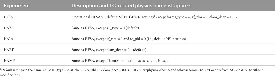
Table 2. Summary of HFSA-based experiments.
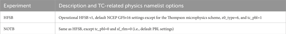
Table 3. Summary of HFSB-based experiments.
Since there are three TC-specific modifications used in the HFSA configuration, three HFSA-based experiments, referred to as HAZ0, HAL0, and HAET, were run, where the respective modifications were not adopted. The HAZ0 experiment uses the default roughness length formulations over open ocean as used in NCEP GFSv16 (default z0_type = 0 in the model namelist) to assess the impact of the TC-specific roughness length formulations on HAFS performance. The HAL0 experiment uses the default settings of the TKE-EDMF PBL scheme as used in NCEP GFSv16 (i.e., sf_rlm = 0 and tc_pbl = 0) to assess the impact of the adjustment of near-surface mixing length in the PBL scheme (sf_rlm = 1) on HAFS performance. The HAET experiment uses the default value of the entrainment rate coefficient (clam_deep = 0.1), which is smaller than that used in the operational HFSA, to assess the impact of the increased entrainment rate. The fourth experiment (HAMP) runs HFSA with the Thompson microphysics scheme instead of the GFDL microphysics scheme to assess the impact of different microphysics schemes on HAFS, although different microphysics schemes were originally intended to add model diversity to HAFS forecasts.
Two TC-specific modifications are used in the HFSB configuration. One is the TC-specific roughness length (z0_type=6) like in HFSA. The other is the TCPBL adjustment in the PBL scheme (tc_pbl = 1). To assess the impact of the TCPBL adjustment in the PBL scheme on HFSB performance, a HFSB-based experiment was run, referred to as NOTB, where the default PBL settings are used, to highlight the impact of the TCPBL adjustment.
For all experiments, the HAFS system is initialized every 6 h with a combined vortex initialization and data assimilation system using data from the NCEP GFSv16 analysis and global data assimilation system. HAFS’s 6-h forecasts from the previous cycle are also used in the initialization for warm cycling (a first-guess of vortex) when the initial Vmax is greater than a threshold (50 kt in HFSA and 40 kt in HFSB). HGFS and each HFSA-based experiment simulated most of the TCs with life cycles longer than 2 days in 2021 and 2022 over the North Atlantic (NATL) basin as listed in Table 4, producing 618 forecast cycles. The HFSB-based experiment simulated the same storms, but also included five NATL storms in 2020 (Table 4), adding 147 cycles to the sample.
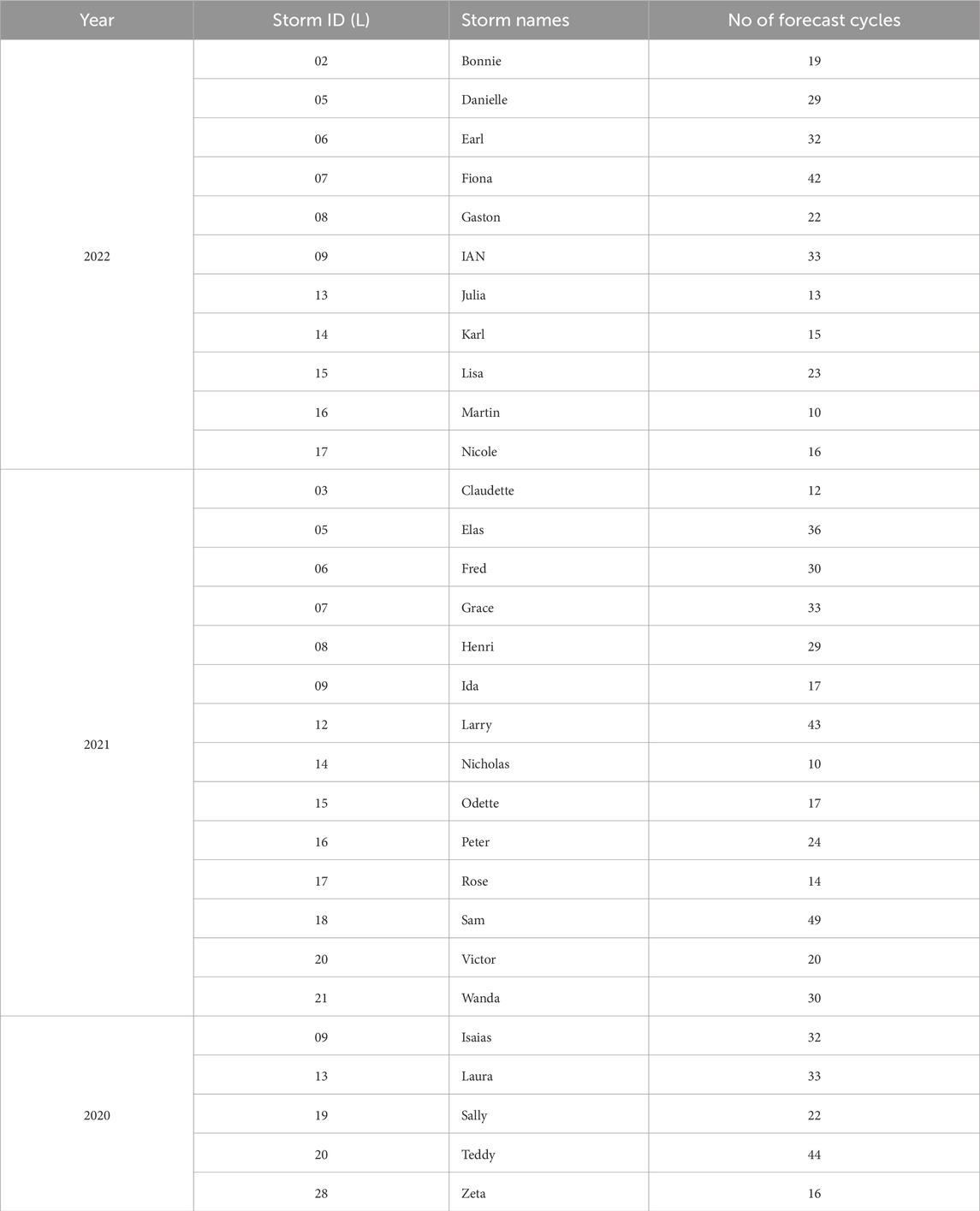
Table 4. List of NATL storms simulated in retrospective HAFS experiments.
The evaluation below focuses on the performance of track, Vmax, and vortex size forecasts by the HAFS experimental runs. NHC’s verification package is used to assess the statistical performance of each experiment against the best-track analysis data.
Figure 1 compares the performance of the HAFS experiments using the NCEP GFSv16 physics package (HGFS, blue lines) and the legacy HWRF (red lines), along with operational configurations (HFSA in purple lines and HFSB in green lines). There are 543 verifiable cycles for this set of 4-run comparison. Compared with HWRF, HGFS has noticeably improved the forecasts of track (Figure 1A) and the radius of 64-kt wind (R64) (Figure 1F) as well as comparable performance in the forecasts of the radii of 34-kt wind (R34) (Figure 1D) and 50-kt wind (R50) (Figure 1E). However, HGFS generates larger root-mean-squared (RMS) errors and biases in Vmax than the legacy HWRF does, with the mean Vmax of HGFS approximately 10 kt weaker than HWRF and the best-track analysis (Figure 1B). In addition, HGFS has degraded the performance in the forecasts of the radius of the surface maximum wind (RMW) (Figure 1C), with larger RMS errors and positive biases than HWRF. This comparison indicates that modifications are needed so that the performance of HAFS is comparable to or better than the then-operational HWRF model at NCEP. As a result, TC-specific modifications are introduced to the two configurations (i.e., HFSA and HFSB) of the operational HAFSv1. Figure 1 shows that the performance of HFSA and HFSB is close to or better than that of HWRF, except for RMW forecasts. Next, we will analyze the impact of each modification on HAFS performance.
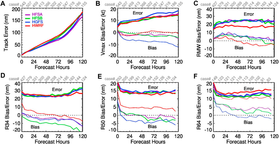
Figure 1. (A) RMS errors of track simulated by HFSA, HFSB, HGFS, and legacy HWRF. RMS errors and biases of (B) Vmax, (C) RMW, (D) R34, (E) R50, and (F) R64.
This section compares the simulated track and Vmax of Hurricane Ian (09 L) from different HAFS experiments to illustrate the impact of the TC-specific modifications or different microphysics schemes on HAFS forecasts.
Hurricane Ian (09 L) was a major Category five hurricane over the NATL basin in 2022. The maximum sustained 10-m wind speed of this hurricane reaches 160 mph, with the central pressure of 937 hPa, just before making landfall in Southwest Florida, United States around 12 UTC on 28 September 2022. Ian originated from a tropical wave. It becomes a numbered storm (09 L) at 12 UTC on 23 September 2022. After that, Ian nearly kept intensifying till 12 UTC on 28 September 2022, with the maximum 10-m wind speed increase reaching 30 kt during 12 h before it reaches peak wind. Ian made three major landfalls during its life cycle. It made its first landfall on the western Cuba as a category three hurricane on 27 September 2022, and its final landfall in South Carolina on 30 September 2022. It was completely dissipated by 12 UTC on 1 October 2022.
The HAFS cycling system in each experiment simulating Hurricane Ian starts from cycle 2022092306 through 2023100106 UTC, initialized every 6 h. Each experiment produced 31 5-day forecasts of track, Vmax, and other atmospheric and oceanic fields.
Figures 2A–E compare the spaghetti plots of the simulated tracks of Hurricane Ian (09 L) from all forecast cycles by different HFSA-based runs, along with the best-track analysis (black solid line). In general, the track forecasts of all runs at lead times beyond 72 h exhibit westward biases, except that some track forecasts initialized on September 23 and 24, 2022 are biased to the east (red lines). Comparing HAZ0, HAL0, and HAET with HFSA shows that the TC-specific modifications do not have major impacts on track forecasts, despite improved track biases in some cycles. Using the Thompson microphysics scheme improves the track forecasts at lead times less than 72 h or 96 h of the cycles initialized on September 23 and 24, 2022 (i.e., less eastward biases) but it degrades the track forecasts at lead times beyond 72 h of the cycles initialized on September 25–28, 2022 (i.e., more westward biases, see red, green, and blue lines). Figures 2F–J compare the spaghetti plots of Vmax forecasts for all cycles. It shows that the modified roughness lengths and mixing length as well as the entertainment rate adjustment do improve the rapid intensification (RI) forecasts initialized on September 23–26, 2022 (red and green lines). HFSA with the Thompson microphysics scheme (HAMP) produces not only stronger Vmax forecasts but also better RI forecasts than that with the GFDL scheme. Figure 3 quantitatively compares the RMS errors and mean biases of track, Vmax, and vortex sizes at different forecast lead times. HAZ0 and HAL0 do not have major changes in the track RMS errors, compared with HFSA, while increasing the entrainment rate (HAET vs. HFSA) does reduce the track RMS errors for lead times beyond 96 h. The run with the Thompson microphysics scheme (HAMP) degrades the track forecast for Hurricane Ian, due to large westward bias as shown in Figure 2. HFSA has smaller RMS errors and biases in Vmax than HAZ0, HAL0, and HAET, indicating improvements by those TC-specific modifications. Noticeably, HAMP has the smallest Vmax biases, although RMS errors are close to those of HFSA. For TC structure verifications, all RMS errors in vortex sizes are very close among the experiments, but differences in the mean sizes from the different experiments are noticeable. For lead times beyond 48 h, using the modified roughness length in HAFS reduces the mean RMW, while adjusting the mixing length and entrainment rate increases the mean RMW, leading to positive RMW bias. The mean R34 decreases with lead time for all experiments, resulting in large negative R34 bias for lead times beyond 96 h. Overall, using the modified roughness length and increasing the entrainment decreases the mean sizes of R34, R50, and R64, respectively. Both adjusting the mixing length and using the Thompson microphysics scheme increase the vortex size.
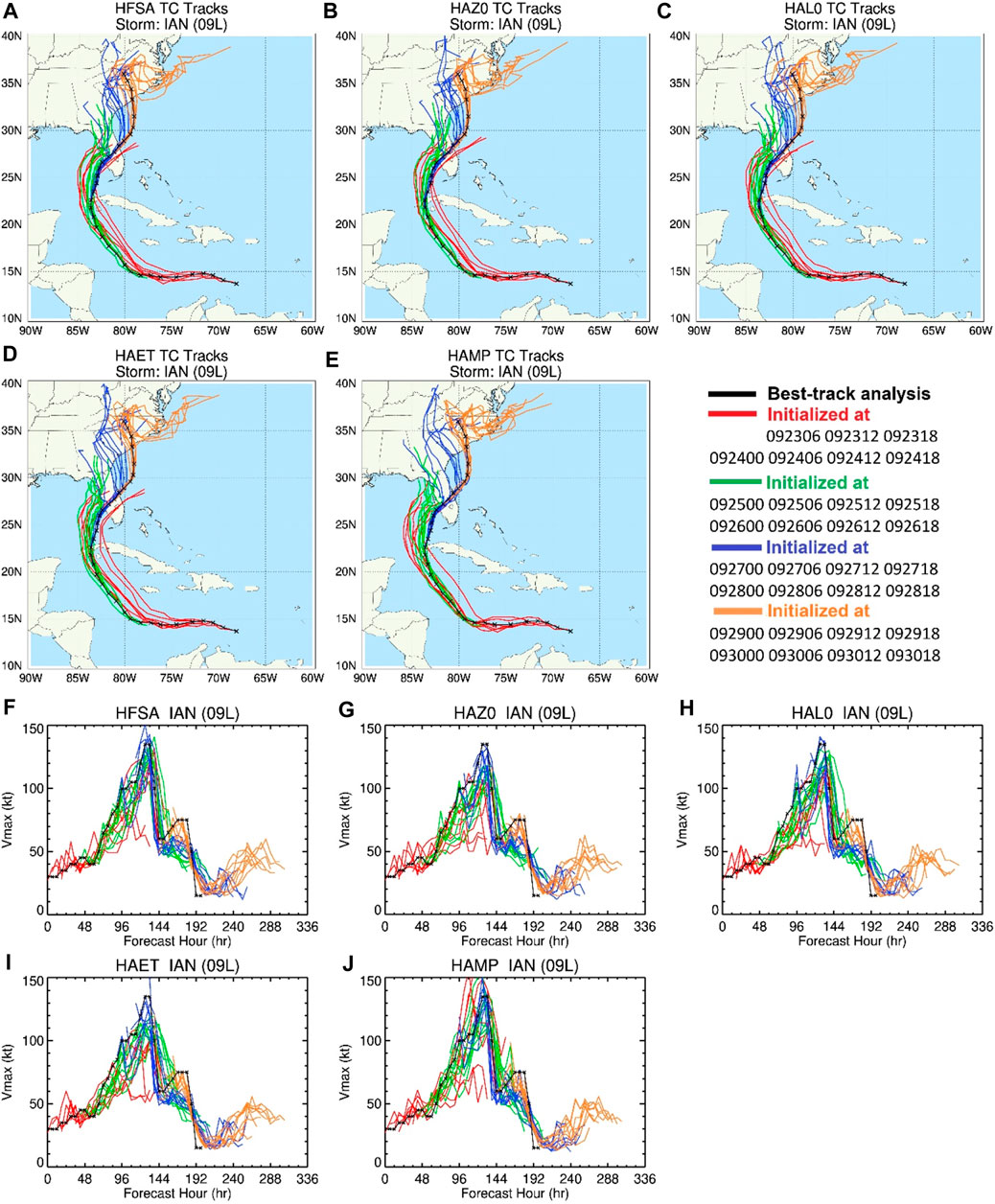
Figure 2. Spaghetti plots of the simulated tracks of Hurricane Ian (09 L) from all forecast cycles (2022092306–093018) of different HFSA-based experiments. (A) HFSA, (B) HAZ0, (C) HAL0, (D) HAET, and (E) HAMP. The black line denotes the best track analysis. Colored lines are for the tracks of different cycles initialized at different days. (F–J) same as (A–E) except for Vmax.
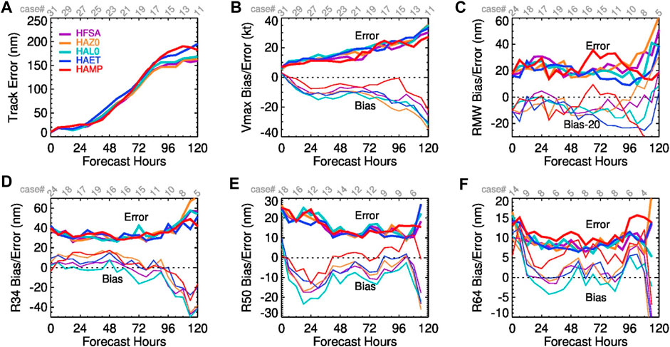
Figure 3. (A) RMS errors of track from the simulated IAN (09 L) cycles from HFSA-based experimental runs, RMS errors and biases of (B) Vmax, (C) RMW, (D) R34, (E) R50, and (F) R64. Note that the bias of RMW minus 20 is shown in (C).
Similarly, Figure 4 shows the spaghetti plots of track and Vmax from all cycles of Hurricane Ian (09 L) in the HFSB and NOTB experiments. Overall, the track forecasts of HFSB and NOTB have westward biases at lead times beyond 72 h, with the former slightly more westward than the latter (Figures 4A, B). Applying the tc_pbl option improves RI in the cycles initialized on September 23–26 (red and green lines in Figures 4C, D). From the analyses of errors and biases, a notable difference is the improvement of Vmax bias with the tc_pbl option (Figure 5B), although track is slightly degraded on day 5 (Figure 5A). There are no major differences in the RMS errors in RMW, R34, R50, and R64. The TCPBL adjustment in HFSB reduces mean R34, but increases mean R50 and R64 sizes; this degrades the R34 and R64 biases, compared with NOTB. This issue could be due to the impact of the reduced value of Lmax in the nest domain as well as zeroing surface-driven mass fluxes for nearly neutral conditions (Chen and Marks, 2024) in HFSB on vortex size.
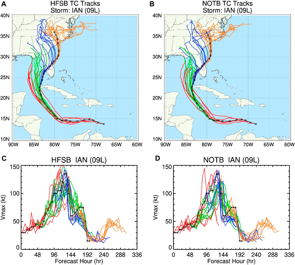
Figure 4. Spaghetti plots of track from all cycles of Hurricane Ian (09 L) simulated by (A) HFSB and (B) NOTB. (C, D) are the same as (A, B) except for Vmax. Same color legend as in Figure 2.
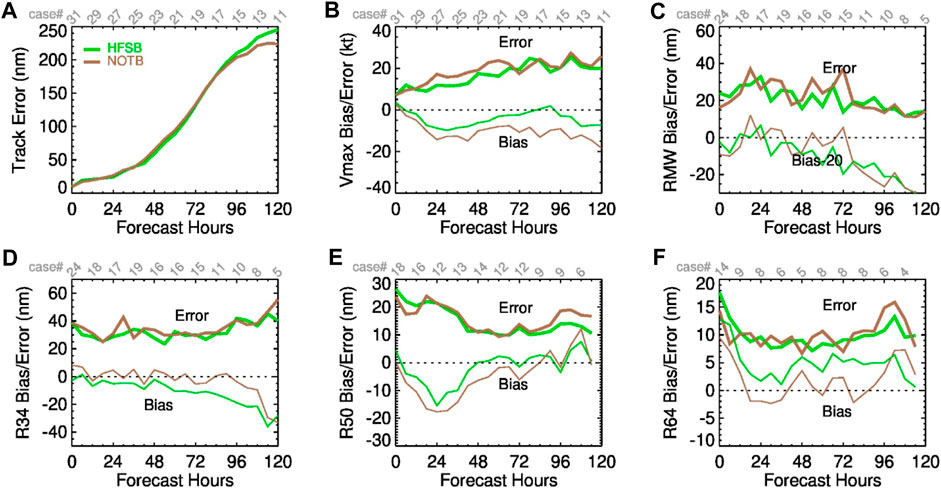
Figure 5. Same as Figure 3 except for HFSB and NOTB.
Based on the criteria of the NHC’s verification package, there are 548 verifiable cycles from all 618 forecast cycles of each HFSA-based experiment. To assess the HAFS performance of weak and strong cycles, a stratified verification analysis is conducted by grouping all verifiable cycles into 367 strong (≥64 kt) and 181 weak (<64 kt) cycles of each HFSA-based experiment based on the maximum Vmax of the best-track analysis during the same 5 days of each cycle. For HFSB-based experiments, there are 684 verifiable cycles from all 765 cycles for each experiment. The verifiable cycles are grouped into 497 strong cycles and 187 weak cycles.
Many investigations have shown that the intensity and structure of a TC simulated by numerical models are sensitive to surface drag coefficients (i.e., Cd and Ck) (e.g., Montgomery et al., 2010; Bryan, 2012; Smith et al., 2014). Ck and Cd characterize the turbulent exchanges of heat and momentum between the ocean and atmosphere in numerical models, respectively. In the atmospheric model of HAFS, the surface fluxes are calculated through the MO similarity theory by specifying the momentum and thermal roughness lengths, rather than directly specifying Cd and Ck values. To compare with observations, we calculate Cd and Ck at 10-m level using the output of HFSA and HAZ0 simulations and display them as a function of 10-m wind speed in Figure 6. The default momentum roughness length over the open ocean in the NCEP GFSv16 model is based on a Charnock relation (Charnock, 1955), capped by a constant (0.0317 m). This relation results in a nearly constant drag coefficient (approximately 0.0025) when 10-m winds are stronger than 30 m/s (Figure 6A). With the modified roughness length described in Section 2.2, the drag coefficient increases generally with 10-m wind speed to approximately 0.0025 from 5 m/s to approximately 30 m/s, then decreases to 0.0016 until 50 m/s, and levels off afterward. This variation is more consistent with the observations (symbols in Figure 6A) than that of the drag coefficient derived from the default momentum roughness length, despite large uncertainty in Cd under strong wind conditions. The values of Ck, derived from the MO similarly theory respectively with the default and modified thermal roughness lengths, are close and much less variable than Cd when 10-m wind speeds are stronger than 5 m/s. For strong winds, Ck is approximately 0.0013–0.0014, despite large uncertainty from observations (Figure 6B).
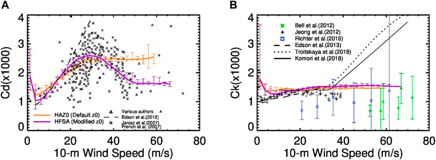
Figure 6. (A) Momentum drag coefficient (Cd) at 10 m as a function of 10-m wind speed used in HAFS experiments and derived from various field or laboratory studies (symbols and black line). Error bars on the purple and orange lines denote the 5th and 95th percentiles in each bin of wind speed of 2 m/s. Triangles represent Cd values from several studies (Bell et al., 2012; Holthuijsen et al., 2012; Bi et al., 2015; Potter et al., 2015; Zhao et al., 2015; Richter et al., 2016); (B) enthalpy exchange coefficient (Ck). Cd and Ck in HAFS are calculated from the HFSA and HAZ0 simulations of Hurricane IAN (09 L), initialized at 2022092806.
Figure 7 compares the HAFS performance using the default (HAZ0) and modified (HFSA) roughness lengths, showing that the modification to the sea surface roughness lengths is necessary for simulating strong TCs. For strong cycles, the largest improvement with the modified roughness lengths is in the Vmax bias, without degrading RMS errors in track (Figure 7A) and Vmax (Figure 7B). While the mean intensities of both HAZ0 and HFSA at all lead times are weaker than those from the best-track analysis, the negative bias on day 5 of HFSA is reduced by 60%, compared with HAZ0. In regard to vortex size, RMS errors and biases in RMW, R34, R50, and R64 near the surface of HFSA are close to those of HAZ0 except that the mean R34 and R50 values of HFSA are reduced. For weak cycles, using the modified roughness lengths does not change the overall performance of HAFS, except for slightly improved track and reduced mean in R34 and R50. This is expected because Cd and Ck in HFSA are very close to those in HAZ0 for weak winds (Figure 6).
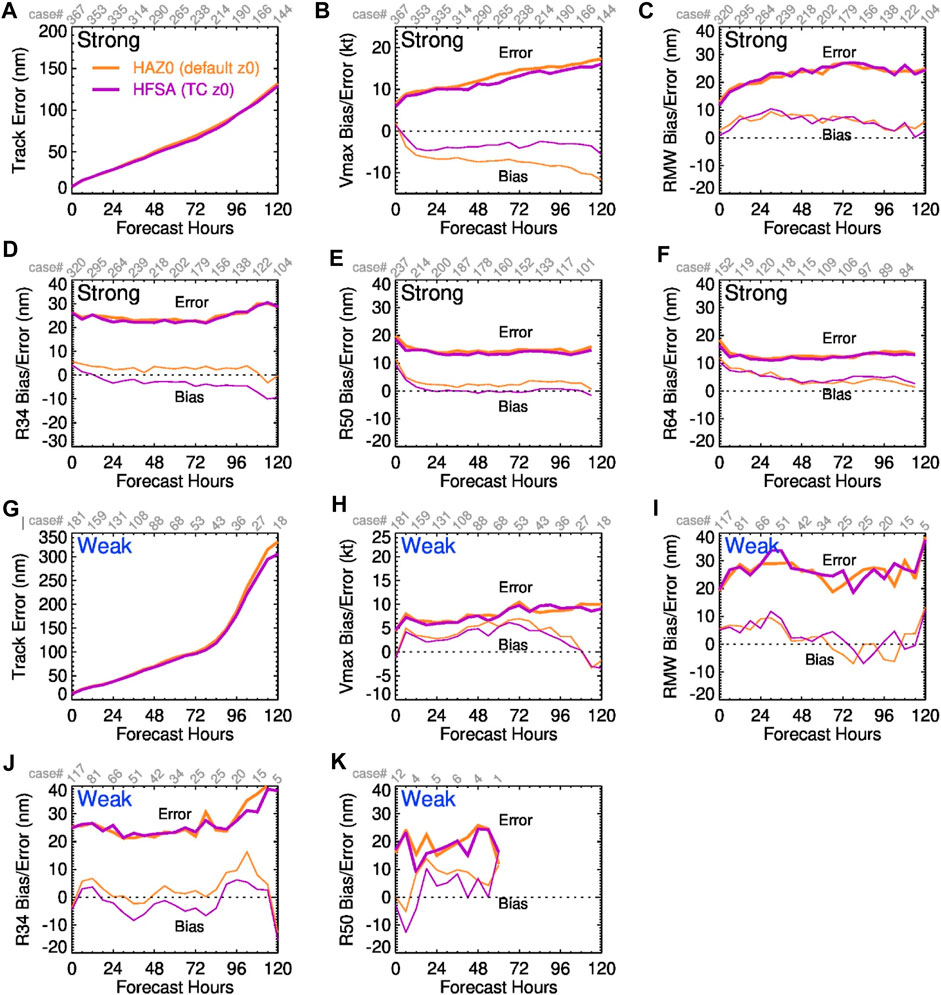
Figure 7. (A) Comparisons of RMS track errors for strong cycles simulated in HFSA and HAZ0 experiments, and RMS errors and biases of (B) Vmax, (C) RMW, (D) R34, (E) R50, (F) R64. (G–K) are the same as (A–E), except for weak cycles. Case count is shown in gray in the upper x-axis.
HFSA and HAL0 experiments are identical except that the options of sf_rlm = 1 and 0 are used in HFSA and HAL0, respectively. With sf_rlm = 1, the vertical mixing length in the TKE-EDMF PBL scheme is modified to make sure it is consistent with the MO similarity theory near the surface (within the level of 5% of PBL height). HAL0 uses the original TKE-EDMF PBL scheme (i.e., sf_rlm = 0). Wang et al. (2023a) described and analyzed the modification and the sensitivity of HAFS performance to different formulations of vertical mixing length. They also showed that the modification improves the vertical profiles of near-surface wind in the eyewall area.
Figure 8 compares the HAFS performance with and without the modification. Compared with HAL0, the RMS errors in track and Vmax of HFSA are slightly reduced for both weak and strong cycles. A more notable improvement is that the negative Vmax bias is reduced by 40%–50% for strong cycles (Figure 8B). The increased mixing length near the surface enhances the downward momentum mixing, and hence strengthens the radial wind to maintain dynamic balance, in favor of vortex intensification. The RMS errors in the vortex sizes of HAL0 and HFSA are close. However, the mean sizes of R34, R50, and R64 in HFSA are increased with the modification; this makes R34 and R50 of HFSA closer to the best-track analysis at all lead times than those of HAL0 (Figures 8C, D) but produces too large R64 (Figure 8F). Despite the differences in mean R34, R50, and R64, the modification does not noticeably change the mean RMW values. For weak cycles, the performances of HAL0 and HFSA are close except that HFSA slightly increases the positive bias of Vmax and reduces the negative R34 bias (Figures 8H, J). As the number of strong cycles is approximately twice that of weak cycles, the modification improves the operational HFSA in general but more efforts are still needed to reduce the positive Vmax bias of weak cycles and positive R64 bias of strong cycles. The detailed analyses on the impact of the modification on storm structure can be found in Wang et al. (2023a).
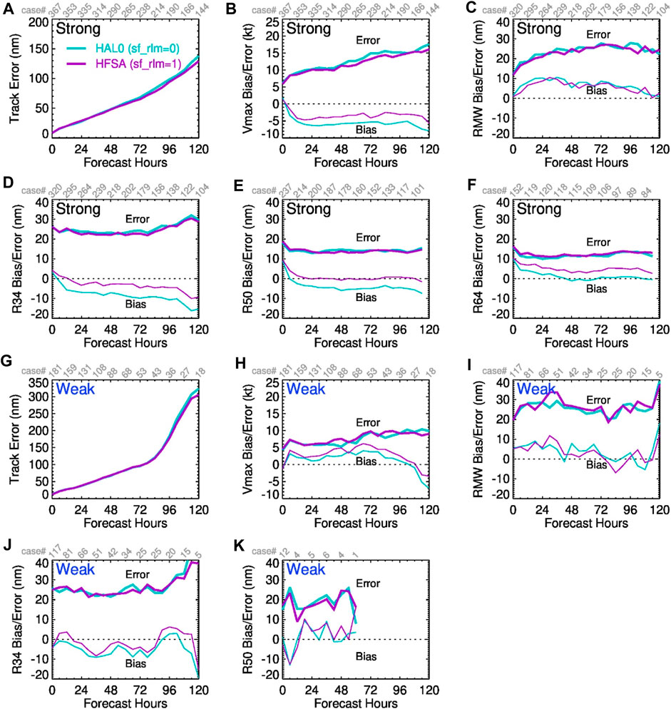
Figure 8. Same as Figure 7, except for HAL0 and HFSA to assess the impact of sf_rlm = 1 option.
The deep convection entrainment rate (Ꜫ) of the scale-aware Simplified Arakawa-Schubert (SAS) convection scheme is formulated as (Han and Pan, 2011; Han et al., 2017),
where z is the height; c a tunable parameter (called clam_deep in the model namelist) whose default value is set to be 0.1 (Han and Pan, 2011; Han et al., 2017); qs and qsb the saturation specific humidity values at the parcel level and the cloud base, respectively; d1 a tunable parameter of O (10−4); RH the environmental relative humidity. Shin et al. (2022) have showed that the storm Vmax is sensitive to this parameter and the overall Vmax forecast can be improved when the c value is increased based on the previous real-time HAFS experiments conducted in the 2020–2022 hurricane seasons. They also found that the simulated storms can respond differently to changes in the entrainment rate of the SAS deep convection scheme. Figure 9 compares the 60 h forecasts of 850-hPa radar reflectivity distributions from HAFS simulations using the c values of 0.1 (C010) and 0.13 (C013), respectively, for Hurricane Teddy initialized at 2020091600 and Hurricane Danielle initialized at 2022090300. For Hurricane Teddy, both C010 and C013 experimental runs produce well-developed strong vortices and do not produce large differences in Vmax and convective structure (Figures 9A–C). However, this is different for Hurricane Danielle simulation (Figure 9D). The storm generated by the C010 experiment exhibits a compact structure with a well-defined eyewall while the C013 experiment produces a relatively weaker and larger storm with more diffusive convective patterns (Figures 9E, F). As described in Shin et al. (2022), changing c and hence different storm environments could cause large differences in the Vmax forecast. Details about the influence of c on the Vmax forecast will be analyzed in a separate paper.
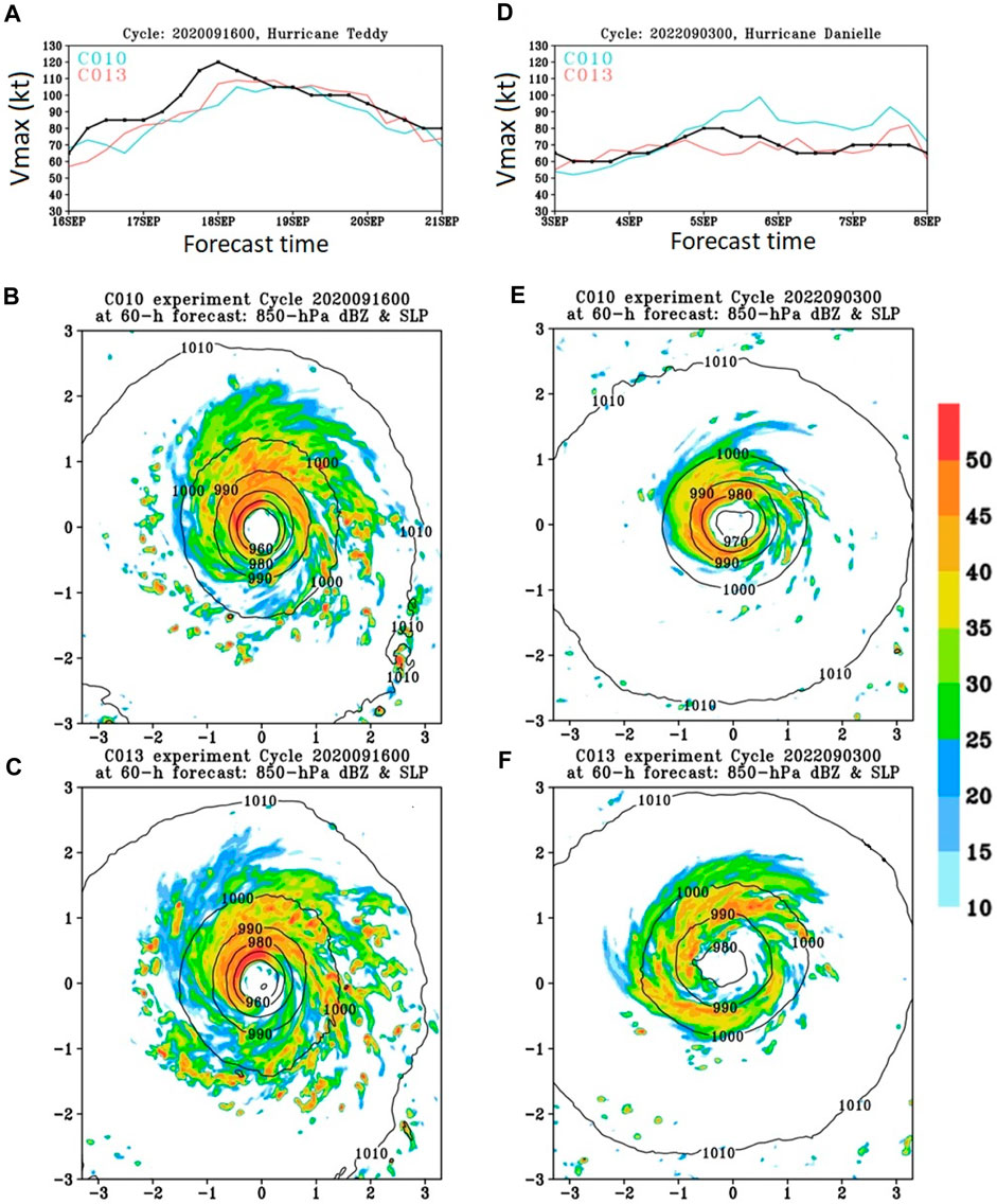
Figure 9. (A) Vmax time series from two HFSA-based experiments (cyan: C010 and red: C013) and from NHC best-track analysis (black) for the Hurricane Teddy simulation initialized at 2020091600. (B) 850-hPa radar reflectivity (shaded: dBZ) and isobar (black contours with 10-hPa interval) from the 60 h forecast of the C010 experiment for the Hurricane Teddy simulation shown in (A). (C) is the same as (B) but from the C013 experiment; (D), (E, F) are the same as (A–C), respectively, but for the Hurricane Danielle simulation initialized at cycle 2022090300. The horizontal and vertical axes are the distance (unit: degree) from the storm center in (B, C, E, F).
Given that increasing c appears to be beneficial for the Vmax forecast, a slightly higher c (clam_deep) value of 0.15 is adopted in the first version of operational HFSA. Figure 10 demonstrates that the operational version of HFSA predicts the storm Vmax better for both strong and weak cycles in terms of RMS errors and biases when 0.15 is used instead of the default value of 0.1. Track RMS errors are also improved. The RMS errors and biases in vortex sizes are nearly unchanged except that the mean R34 of HFSA is slightly smaller than that of HAET.
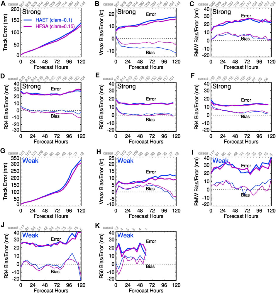
Figure 10. Same as Figure 7, except for HAET (clam_deep = 0.1) and HFSA (clam_deep = 0.15) to assess the impact of the increased entertainment rate.
Given the uncertainty in physics schemes, the purpose of using different microphysics schemes in HFSA and HFSB configurations is to increase the forecast diversity in addition to other differences in both configurations (Section 2). To highlight the impact of different microphysics schemes on HAFS performance, we run HFSA with the Thompson microphysics scheme (HAMP) replacing the GFDL microphysics scheme. In the literature, numerous studies have reported that varying cloud microphysics assumptions, resulting in different thermal and dynamical effects induced by phase changes, can have major impacts on the intensity of TCs simulated by mesoscale models with different microphysics schemes (see a review paper by Tao et al. (2011), and references therein). Fovell et al. (2009) showed that TC track forecast may also be influenced by different microphysics assumptions via cloud–radiative interaction.
Figure 11 shows the statistical errors in track, Vmax, and vortex size of TCs simulated by the HAFS model with GFDL (HFSA, purple lines) and Thompson (HAMP, red lines) microphysics schemes. The simulations with the two microphysics schemes have noticeable impacts on track and Vmax. For strong cycles, it appears that HAMP produces larger track errors for lead times beyond 48 h than HFSA, while it produces smaller Vmax RMS errors for nearly all lead times with larger mean intensities (and smaller negative biases) within 48 h. The RMW errors and biases of HAMP are generally close to those of HFSA, except that HAMP has slightly smaller RMW errors and smaller mean RMW for the lead times beyond 72 h. The RMS errors in R34, R50, and R64 from both runs are also close, but HAMP produces smaller mean values of R34 and R50 than HFSA. The mean R64 values of HAMP are larger than those of HFSA for the lead times within 60 h, and smaller afterward. For weak cycles, HAMP has smaller track errors for nearly all lead times, especially for the lead times beyond 84 h. The RMS errors and biases in Vmax and vortex size of HAMP are generally close to those of HFSA.
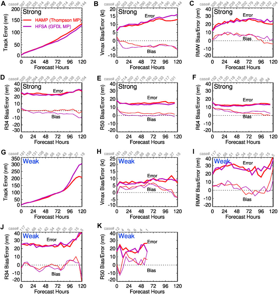
Figure 11. Same as Figure 7, except for HAMP and HFSA to assess the impact of different microphysics schemes.
As described in Section 2, major differences in the two microphysics schemes are in the treatments of ice processes and the number concentrations of hydrometeors. In-depth comparisons of the impact of the two schemes are beyond the scope of this document. Here we only show the vertical distributions of azimuthally-averaged mixing ratios of hydrometeors from the two schemes in one cycle simulation of Hurricane Fiona (07 L) as an example to highlight differences in hydrometeors simulated by the two schemes (Figure 12). An apparent difference in the distributions of hydrometeors is that the Thompson microphysics scheme produces much more snow than the GFDL microphysics scheme and less cloud ice and graupel, although we do not have sufficient observational data to verify those results. Different treatments of the conversion of water vapor and hydrometeors are likely to generate different condensational heating rates and cloud-radiative interactions, affecting the simulations of the Vmax and track of TCs. Some case studies also showed that using the Thompson microphysics scheme in HAFS tends to produce a slightly taller vortex than using the GFDL microphysics scheme. The Thompson scheme has notably weaker reflectivity than the GFDL microphysics scheme aloft probably due to the larger bias of snow and lack of small ice particles being lifted far above the freezing level. In addition, HAFS with the GFDL microphysics scheme has slightly higher vertical velocity maxima aloft. For detailed analyses, see Hazelton et al. (2023b).
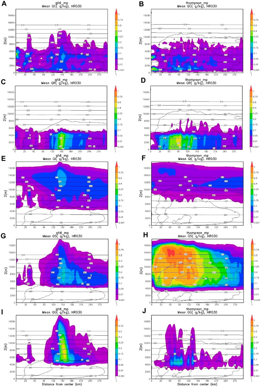
Figure 12. Vertical distributions of azimuthally-averaged mixing ratios (g/kg) of hydrometeors at the forecast time of 30 h for Hurricane Fiona (07 L) simulated by HAFS using the GFDL (left column) and Thompson (right column) microphysics schemes with the same initial conditions at 2022092106. (A,B) liquid cloud, (C,D) rain, (E,F) cloud ice, (G,H) snow, and (I,J) graupel. Horizontal lines are the contours of temperature (K) and curved lines are the contours of tangential winds.
The configuration of the NOTB run is identical to that of the HFSB run except that the default PBL scheme (tc_pbl=0) is used in NOTB, while the TCPBL adjustment in the PBL scheme (tc_pbl = 1) is used in HFSB. For strong cycles, the TCPBL adjustment improves the Vmax bias by 50% (Figure 13B), despite a slight increase in track errors for lead times beyond 96 h (Figure 13A). It does not have major impacts on the RMS errors in vortex sizes (RMW, R34, R50, and R64), but results in some improvements to mean biases in RMW, R50, and R64. One noticeable impact is on the mean R34 bias, as shown in Figure 13D. Both HFSB and NOTB have negative biases in R34. Using the TCPBL adjustment increases the negative R34 bias with forecast time. This issue is primarily attributable to the setting of turning off surface-driven mass fluxes (Mu) where the surface stability parameter is greater than −0.5 (Chen and Marks, 2024). The objective of this setting is to retain Mu only in convective boundary layers, as Mu essentially represents buoyant thermal plumes in convective boundary layers. Exploring a suitable threshold of surface stability parameter differentiating buoyancy-driven and shear-driven boundary layers is currently underway. For weak cycles, the impact of the TCPBL adjustment is small as expected, except that track errors are increased for the lead times beyond 72 h.
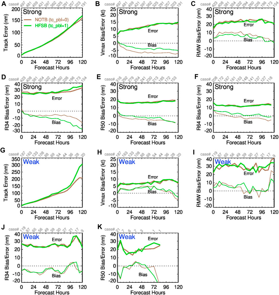
Figure 13. Same as Figure 7, except for NOTB and HFSB to assess the impact of tc_pbl=1 option in HFSB.
Other testing has also shown that the TCPBL adjustment improves the simulated structure of TCs in HAFS (Chen et al., 2022; Chen et al., 2023). An examination of the relative impacts of TCPBL adjustment and the Thompson microphysics scheme in HFSB retrospective forecasts has also demonstrated that the TCPBL adjustment was critical to the improved detection of RI in HFSB (Hazelton et al., 2023a; Hazelton et al., 2023b). Composite structures have shown that the TCPBL adjustment increases the boundary layer inflow strength, leading to more compact and robust vortices that spin up more quickly (Hazelton et al., 2023a; Hazelton et al., 2023b).
Numerous early investigations have shown that the Vmax of a TC is closely related to its minimum central pressure (e.g., Holland, 2008 and references therein), called pressure-wind relation. Near the TC center, the horizontal pressure gradient and centrifugal forces are approximately balanced. The pressure-wind relation is a useful metric to evaluate the model performance. Figure 14 presents the fitted pressure-wind relationships from all the experiments and the best-track analysis, respectively. It is seen that all HAFS experiments generally produce a weaker Vmax than the best-track analysis does under a given central pressure. This is consistent with the general negative biases in Vmax of HAFS runs as shown in Section 3.2. In the HFSA-based experiments, using the Thompson microphysics scheme (HAMP) and the modified mixing length near the surface (HAL0) do not significantly change the pressure-wind relation, as compared with that of HFSA. However, using the modified roughness length and increased entrainment rate can noticeably improve the pressure-wind relation for intensities stronger than 80 kt, with an increased Vmax at a given central pressure lower than 960 hPa, respectively (HFSA vs. HAZ0, and HFSA vs. HAET). For intensities weaker than 80 kt, all experimental runs produce nearly the same pressure-wind relation. In the HFSB-based experiment, the TCPBL adjustment in the PBL scheme (HFSB) improves the pressure-wind relation, compared with that without the adjustment (NOTB). Specifically, the TCPBL allows greater Vmax at a given central pressure when the central pressure is lower than 980 hPa (or for Vmax stronger than 60 kt).
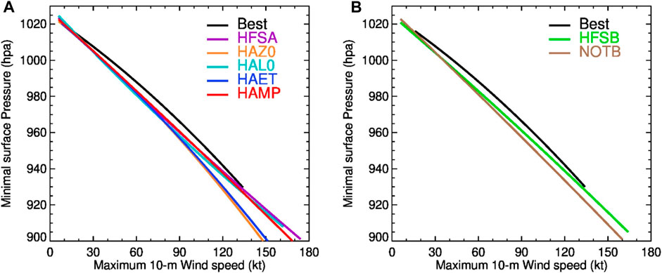
Figure 14. Fitted Pressure-wind relations of (A) HFSA-based experiments and (B) HFSB-based experiments. Black lines are fitted from the best track analysis.
The probability of detection (POD) index of the observed RI events and false alarm ratio (FAR) index of the forecasted RI events are used to characterize the model performance in predicting RI events. We calculated POD and FAR indices for the observed and forecasted RI events, respectively, by aggregating the forecasts at all lead times of all cycles in each experiment. Figure 15A shows the performance diagram summarizing POD, success ratio (SR = 1-FAR), and critical success index (CSI, also known as threat score) of each experiment. The POD values of all HAFS experiments are smaller than their respective SR values, although both POD and SR are not high. Compared with HAZ0, using the modified roughness lengths in HFSA increases POD by 15% and reduces FAR by 5%. Likewise, the increased entrainment rate leads to an increased POD by 12% and a reduced FAR by 3% (HAET vs. HFSA). Adjusting the near-surface mixing length increases POD by 9% without increasing FAR (HAL0 vs. HFSA). Using the Thompson microphysics scheme in HFSA further increases POD by 7% and reduces FAR by 14% (HAMP vs. HFSA), improving FAR more than POD. In the HFSB-based experiment, using the TCPBL adjustment increases POD by 8% without increasing FAR (NOTB vs. HFSB). All TC-specific modifications increase POD and reduce or do not increase FAR in both HFSA and HFSB; this improves the CSI values of RI forecasts. The improvement of POD is more noticeable than that of FAR. Nevertheless, the POD is still low for both HFSA and HFSB; this needs to be addressed in future upgrades.
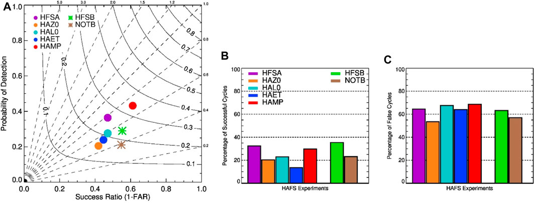
Figure 15. (A) Performance diagram of RI forecasts by different experimental runs. The critical intensity increase for RI is 30 kt per 24 h. Dashed lines are bias scores. Solid labeled contours are critical success indexes (also known as threat score). (B) The percentage of the cycles in each HAFS experiment successfully detecting the observed RI events during individual 5-day forecasts. (C) Same as (B), except for the cycles falsely predicting RI events.
In addition, we analyzed POD and FAR during each single 5-day forecast period, referred to as POD5 and FAR5, respectively, to assess the performance of RI forecasts of each cycle (Wang et al., 2023c). A forecast cycle is thought to successfully detect the observed RI events if POD5 is larger than 0.5, and falsely predicts RI events if FAR5 is larger than 0.5. Figures 15B, C show the percentages of the cycles successfully detecting the observed RI events and falsely predicting RI events during 5-day forecasts in each experiment. All TC-specific modifications do improve the ratio of the cycles successfully detecting the observed RI events. They also slightly reduce the ratio of the cycles falsely predicting RI events except for the modified roughness lengths and the TCPBL adjustment increasing the number of false RI prediction cycles. Comparing HAMP with HFSA, using the Thompson microphysics scheme slightly decreases the percentage of successful cycles and increases the percentage of false cycles.
Future HAFS upgrades focus mainly on increasing the diversity between HFSA and HFSB, improving the forecasts of rapid changes in intensity, particularly for NATL basin, reducing intensity forecast errors at long lead times, and improving vortex structure forecasts. Both HFSA and HFSB are capable of forecasting rapid changes in Vmax, but they still suffer from high biases in Vmax, false prediction of RI, underpredicting Vmax changes, and the timing of onset of rapid intensity changes. These forecasting challenges also remain for other regional dynamic models as summarized by Zhang et al. (2023). These are one of the major challenges for the further development of HAFS. For example, both HFSA and HFSB predicted RI of hurricane Lee (13 L) 12–24 h later than the best-track analysis for the cycles initialized earlier than 2023090706, and struggled to predict rapid weakening after the intensification period. This led to large intensity errors and biases for lead times beyond 24 h, resulting in underperformance compared to the legacy HWRF model. Although the reasons for the underperforming forecast of rapid intensity changes are not clear yet, preliminary experimental studies suggested that it could be related to model dynamics and physics (Liu et al., 2023; Zhang and Zhang, 2023). Another challenge is to improve the structure of the forecasted vortex. As shown in Figure 1, RMW errors and biases of HAFS are still lager than those of the legacy HWRF.
To further improve physics schemes in the operational HAFS, we will continue to explore the upgraded physics schemes for NCEP GFS in TC simulations using HAFS, including the improved PBL and convection schemes in strong shear environment conditions (Han et al., 2021; Han et al., 2024) as well as the next version of the GFDL microphysics scheme. Given the critical role of the PBL in TC forecasts, the MYNN-EDMF PBL scheme (Olson et al., 2019), which has been extensively tested in the regional Rapid Refresh Forecast System at NCEP and can be well performed in simulating hurricane boundary layers (Chen and Bryan, 2021; Chen, 2022), is also worth testing in HAFS with some modifications for strong wind conditions. Despite the high horizontal resolution used in HAFS, convection schemes still play an important role in modulating both intensity and track of TCs in HAFS. Therefore, other convection schemes such as Tiedtke cumulus scheme (Tiedtke, 1989) and Grell-Freitas scheme (Freitas et al., 2021) are being tested in HAFS. Other upgrade plans include the use of NOAH-MP (Niu et al., 2011) in HAFS, testing different options in the advection scheme, and testing the physics-dynamics interaction.
Research efforts should be made to further improve the capability of a single physics scheme applied to multiple scales, i.e., scale-awareness, and to test model parameters such as the entrainment rate in convection schemes and diffusivity in PBL schemes as well as different treatments of microphysical processes for TC scenarios. It is worth mentioning that the entrainment rate is an important parameter in convection schemes and has noticeable impacts on TC intensity forecasts as shown in Section 3.2.3. There are many studies on how to improve the entrainment parameterization (e.g., Zhang et al., 2016; Xu et al., 2021; Villalba-Pradas and Tapiador, 2022). It is warranted to test the impact of different entrainment rate parameterizations on TC forecasts of HAFS. In addition, the role of microphysical processes in TC simulations should be further investigated, given that the performance of HAFS is sensitive to microphysics schemes it chooses. It is beneficial for HAFS to test the sensitivity of TC simulations in HAFS to different treatments of microphysical processes such as mixing evaporation and autoconversion processes and their relationships (Liu et al., 2023; Lu et al., 2023).
This paper describes the physics schemes used in the first version of operational HAFS. The physics schemes are the same as those used in NCEP GFS version 16, with the exception of four TC-specific modifications and a different microphysics scheme in one of the two HAFSv1 configurations. The four modifications include (1) the observation-based sea-surface roughness lengths, (2) increased near-surface mixing length in the PBL, (3) increased entrainment rate in the SAS deep convection scheme, and (4) adjustments for TC PBL including reduced maximum allowable mixing length, the adjusted two coefficients in the eddy viscosity and TKE dissipation term, and tapering nonlocal mass fluxes in high-wind conditions. Experiments show that all of the modifications improve Vmax forecasts, particularly for mean Vmax biases of strong cycles, without degrading track forecasts. The modifications have nearly negligible impacts on RMS errors in R34, R50, and R64, but have noticeable impacts on mean biases, with the largest impact on mean R34 bias. RMW errors and biases are not affected by the modifications. All modifications improve the POD of the observed RI events and FAR of the forecast RI events. The improvement of the POD is larger than that of the FAR, although the POD is still low and the FAR is still high. The use of the Thomspson microphysics scheme in one HAFSv1 configuration was originally intended to increase the diversity of HAFS forecasts between the two configurations. However, the experiment indicates that using the Thompson microphysics scheme can greatly improve HFSA intensity forecasts for both strong and weak cycles as well as POD and FAR of RI forecasts.
In addition to the analyses of track and intensity as presented in this paper, it is worth further investigating the impact of physics schemes and their modifications on the structure of TCs simulated by HAFS. This is needed to identify issues common for all models or specific to HAFS. Priority issues to be addressed include the over prediction of intensity in low shear environment, RI onset timing, large cycle-to-cycle variability, and other common issues of regional dynamic models identified by forecasters (Wang et al., 2023b; Zhang et al., 2023). Future work on the HAFS physics package includes:
(1) Testing the upgraded GFS physics schemes in HAFS configurations and making adjustments if necessary.
(2) Exploring other existing PBL and convection schemes in UFS suitable for TC simulations.
(3) Developing new modifications or schemes tailored to HAFS based on research efforts such as improving scale-awareness and sensitivities of HAFS simulations to model parameters (e.g., entrainment rate, diffusivity, and others) and to different treatments of microphysical processes.
The raw data supporting the conclusion of this article will be made available by the authors, without undue reservation.
WW: Conceptualization, Formal Analysis, Investigation, Methodology, Visualization, Writing–original draft, Writing–review and editing. JH: Conceptualization, Writing–original draft, Writing–review and editing. JuS: Conceptualization, Formal Analysis, Investigation, Writing–original draft, Writing–review and editing. XC: Conceptualization, Formal Analysis, Investigation, Writing–original draft, Writing–review and editing. AH: Formal Analysis, Investigation, Methodology, Writing–original draft, Writing–review and editing. LZ: Formal Analysis, Investigation, Writing–original draft, Writing–review and editing. H-SK: Investigation, Methodology, Writing–original draft, Writing–review and editing. XL: Investigation, Writing–original draft, Writing–review and editing. BL: Formal Analysis, Investigation, Methodology, Writing–original draft, Writing–review and editing. QL: Formal Analysis, Investigation, Writing–original draft, Writing–review and editing. JoS: Investigation, Writing–original draft, Writing–review and editing. RS: Investigation, Writing–original draft, Writing–review and editing. WZ: Formal Analysis, Investigation, Writing–original draft, Writing–review and editing. ZZ: Conceptualization, Formal Analysis, Funding acquisition, Investigation, Methodology, Project administration, Resources, Supervision, Writing–original draft, Writing–review and editing. FY: Conceptualization, Formal Analysis, Funding acquisition, Investigation, Methodology, Project administration, Resources, Supervision, Writing–review and editing, Writing–original draft.
The author(s) declare that financial support was received for the research, authorship, and/or publication of this article. XC was supported by the National Oceanic and Atmospheric Administration Grants NA23OAR4590380 and NA21OAR4320190. AH was supported by NOAA grants NA19OAR0220187 and NA22OAR4050668D.
The authors thank Mary Hart, Drs. Jiayi Peng, and Lydia Stefanova providing comments and suggestions on the manuscript during EMC internal review.
The authors declare that the research was conducted in the absence of any commercial or financial relationships that could be construed as a potential conflict of interest.
All claims expressed in this article are solely those of the authors and do not necessarily represent those of their affiliated organizations, or those of the publisher, the editors and the reviewers. Any product that may be evaluated in this article, or claim that may be made by its manufacturer, is not guaranteed or endorsed by the publisher.
1Kim, H.-S., Liu, B., Thomas, B., Rosen, D., Wang, W., Hazelton, A., et al. (2024). Ocean component of the first operational version of hurricane analysis and forecast system: HYbrid coordinate Ocean model (HYCOM). Front. Earth Sci. in review.
Aligo, E. A., Ferrier, B., and Carley, J. R. (2018). Modified NAM microphysics for forecasts of deep convective storms. Mon. Weather Rev. 146 (12), 4115–4153. doi:10.1175/MWR-D-17-0277.1
Alpert, J., Kanamitsu, M., Caplan, P. M., Sela, J. G., White, G. H., and Kalnay, E. (1988). “Mountain induced gravity wave drag parameterization in the nmc medium-range forecast model,” in Eighth conf. On numerical weather prediction (Baltimore, MD: Amer. Meteor. Soc.).
Beljaars, A. C. M., Brown, A. R., and Wood, N. (2004). A new parametrization of turbulent orographic form drag. Q. J. R. Meteorological Soc. 130, 1327–1347. doi:10.1256/qj.03.73
Bell, M. M., Montgomery, M. T., and Emanuel, K. A. (2012). Air–Sea enthalpy and momentum exchange at major hurricane wind speeds observed during CBLAST. J. Atmos. Sci. 69 (11), 3197–3222. doi:10.1175/JAS-D-11-0276.1
Bender, M. A., Ginis, I., Tuleya, R., Thomas, B., and Marchok, T. (2007). The operational GFDL coupled hurricane–ocean prediction system and a summary of its performance. Mon. Weather Rev. 135 (12), 3965–3989. doi:10.1175/2007MWR2032.1
Bi, X., Gao, Z., Liu, Y., Liu, F., Song, Q., Huang, J., et al. (2015). Observed drag coefficients in high winds in the near offshore of the South China Sea. J. Geophys. Res. Atmos. 120 (13), 6444–6459. doi:10.1002/2015JD023172
Biswas, M. K., Abarca, S., Bernardet, L., Ginis, I., Grell, E., Iacono, M., et al. (2018). Hurricane weather research and forecasting (HWRF) model: 2018 scientific documentation. Available at: https://dtcenter.org/sites/default/files/community-code/hwrf/docs/scientific_documents/HWRFv4.0a_ScientificDoc.pdf.
Bleck, R. (2002). An oceanic general circulation model framed in hybrid isopycnic-Cartesian coordinates. Ocean. Model. 4 (1), 55–88. doi:10.1016/S1463-5003(01)00012-9
Bleck, R., Halliwell, G. R., Wallcraft, A. J., Carroll, S., Kelly, K., and Rushing, K. (2002). HYbrid Coordinate Ocean Model (HYCOM) user's manual: details of the numerical code. HYCOM, version 2, 1–211.
Boscheri, W., and Dumbser, M. (2014). A direct Arbitrary-Lagrangian–Eulerian ADER-WENO finite volume scheme on unstructured tetrahedral meshes for conservative and non-conservative hyperbolic systems in 3D. J. Comput. Phys. 275, 484–523. doi:10.1016/j.jcp.2014.06.059
Bryan, G. H. (2012). Effects of surface exchange coefficients and turbulence length scales on the intensity and structure of numerically simulated hurricanes. Mon. Weather Rev. 140 (4), 1125–1143. doi:10.1175/MWR-D-11-00231.1
Charnock, H. (1955). Wind stress on a water surface. Q. J. R. Meteorological Soc. 81 (350), 639–640. doi:10.1002/qj.49708135027
Chassignet, E. P., Smith, L. T., Halliwell, G. R., and Bleck, R. (2003). North atlantic simulations with the hybrid coordinate Ocean Model (HYCOM): impact of the vertical coordinate choice, reference pressure, and thermobaricity. J. Phys. Oceanogr. 33 (12), 2504–2526. doi:10.1175/1520-0485(2003)033<2504:NASWTH>2.0.CO;2
Chen, J.-H., and Lin, S.-J. (2011). The remarkable predictability of inter-annual variability of Atlantic hurricanes during the past decade. Geophys. Res. Lett. 38 (11). doi:10.1029/2011GL047629
Chen, J.-H., and Lin, S.-J. (2013). Seasonal predictions of tropical cyclones using a 25-km-Resolution general circulation model. J. Clim. 26 (2), 380–398. doi:10.1175/jcli-d-12-00061.1
Chen, X. (2022). How do planetary boundary layer schemes perform in hurricane conditions: a comparison with large-eddy simulations. J. Adv. Model. Earth Syst. 14 (10), e2022MS003088. doi:10.1029/2022MS003088
Chen, X., Andronova, N., Van Leer, B., Penner, J. E., Boyd, J. P., Jablonowski, C., et al. (2013). A control-volume model of the compressible euler equations with a vertical Lagrangian coordinate. Mon. Weather Rev. 141 (7), 2526–2544. doi:10.1175/mwr-d-12-00129.1
Chen, X., and Bryan, G. H. (2021). Role of advection of parameterized turbulence kinetic energy in idealized tropical cyclone simulations. J. Atmos. Sci. 78 (11), 3593–3611. doi:10.1175/JAS-D-21-0088.1
Chen, X., Bryan, G. H., Hazelton, A., Marks, F. D., and Fitzpatrick, P. (2022). Evaluation and improvement of a TKE-based eddy-diffusivity mass-flux (EDMF) planetary boundary layer scheme in hurricane conditions. Weather Forecast. 37 (6), 935–951. doi:10.1175/waf-d-21-0168.1
Chen, X., Bryan, G. H., Zhang, J. A., Cione, J. J., and Marks, F. D. (2021). A framework for simulating the tropical cyclone boundary layer using large-eddy simulation and its use in evaluating PBL parameterizations. J. Atmos. Sci. 78 (11), 3559–3574. doi:10.1175/jas-d-20-0227.1
Chen, X., Hazelton, A., Marks, F. D., Alaka, G. J., and Zhang, C. (2023). Performance of an improved TKE-based eddy-diffusivity mass-flux (EDMF) PBL scheme in 2021 hurricane forecasts from the hurricane analysis and forecast system. Weather Forecast. 38 (2), 321–336. doi:10.1175/WAF-D-22-0140.1
Chen, X., and Marks, F. D. (2024). Parameterizations of boundary layer mass fluxes in high-wind conditions for tropical cyclone simulations. J. Atmos. Sci. 81, 77–91. doi:10.1175/jas-d-23-0086.1
Choi, H.-J., and Hong, S.-Y. (2015). An updated subgrid orographic parameterization for global atmospheric forecast models. J. Geophys. Res. Atmos. 120 (24), 12445–12457. doi:10.1002/2015JD024230
Dong, J., Liu, B., Zhang, Z., Wang, W., Mehra, A., Hazelton, A. T., et al. (2020). The evaluation of real-time hurricane analysis and forecast system (HAFS) stand-alone regional (SAR) model performance for the 2019 atlantic hurricane season. Atmosphere 11 (6), 617. doi:10.3390/atmos11060617
Edson, J. B., Jampana, V., Weller, R. A., Bigorre, S. P., Plueddemann, A. J., Fairall, C. W., et al. (2013). On the exchange of momentum over the open ocean. J. Phys. Oceanogr. 43 (8), 1589–1610. doi:10.1175/JPO-D-12-0173.1
Ek, M. B., Mitchell, K. E., Lin, Y., Rogers, E., Grunmann, P., Koren, V., et al. (2003). Implementation of Noah land surface model advances in the National Centers for Environmental Prediction operational mesoscale Eta model. J. Geophys. Res. Atmos. 108 (D22). doi:10.1029/2002JD003296
Fairall, C. W., Bradley, E. F., Hare, J. E., Grachev, A. A., and Edson, J. B. (2003). Bulk parameterization of air–sea fluxes: updates and verification for the COARE algorithm. J. Clim. 16 (4), 571–591. doi:10.1175/1520-0442(2003)016<0571:BPOASF>2.0.CO;2
Ferrier, B. S., Jin, Y., Lin, Y., Black, T., Rogers, E., and DiMego, G. (2002). Implementation of a new grid-scale cloud and precipitation scheme in the NCEP Eta model. 19th conf. On weather analysis and forecasting/15th conf. On numerical weather prediction (San Antonio, TX: American Meteorology Society).
Field, P. R., Hogan, R. J., Brown, P. R. A., Illingworth, A. J., Choularton, T. W., and Cotton, R. J. (2005). Parametrization of ice-particle size distributions for mid-latitude stratiform cloud.
Fovell, R. G., Corbosiero, K. L., and Kuo, H.-C. (2009). Cloud microphysics impact on hurricane track as revealed in idealized experiments. J. Atmos. Sci. 66 (6), 1764–1778. doi:10.1175/2008JAS2874.1
Freitas, S. R., Grell, G. A., and Li, H. (2021). The Grell–Freitas (GF) convection parameterization: recent developments, extensions, and applications. Geosci. Model Dev. 14 (9), 5393–5411. doi:10.5194/gmd-14-5393-2021
French, J. R., Drennan, W. M., Zhang, J. A., and Black, P. G. (2007). Turbulent fluxes in the hurricane boundary layer. Part I: momentum flux. J. Atmos. Sci. 64 (4), 1089–1102. doi:10.1175/JAS3887.1
Gopalakrishnan, S., Hazelton, A., and Zhang, J. A. (2021). Improving hurricane boundary layer parameterization scheme based on observations. Earth Space Sci. 8 (3), e2020EA001422. doi:10.1029/2020EA001422
Han, J., and Bretherton, C. S. (2019). TKE-based moist eddy-diffusivity mass-flux (EDMF) parameterization for vertical turbulent mixing. Weather Forecast. 34 (4), 869–886. doi:10.1175/waf-d-18-0146.1
Han, J., Li, W., Yang, F., Strobach, E., Zheng, W., and Sun, R. (2021). Updates in the NCEP GFS cumulus convection, vertical turbulent mixing, and surface layer physics. Office note (National Centers Environ. Predict. (U.S.)) 505, 18pp. doi:10.25923/cybh-w893
Han, J., and Pan, H.-L. (2011). Revision of convection and vertical diffusion schemes in the NCEP global forecast system. Weather Forecast. 26 (4), 520–533. doi:10.1175/WAF-D-10-05038.1
Han, J., Peng, J., Li, W., Wang, W., Zhang, Z., Yang, F., et al. (2024). Updates in the NCEP GFS PBL and convection models with environmental wind shear effect and modified entrainment and detrainment rates and their impacts on the GFS hurricane and CAPE forecasts. Weather Forecast. 39 (4), 679–688. doi:10.1175/waf-d-23-0134.1
Han, J., Wang, W., Kwon, Y. C., Hong, S.-Y., Tallapragada, V., and Yang, F. (2017). Updates in the NCEP GFS cumulus convection schemes with scale and aerosol awareness. Weather Forecast. 32 (5), 2005–2017. doi:10.1175/waf-d-17-0046.1
Han, J., Witek, M. L., Teixeira, J., Sun, R., Pan, H.-L., Fletcher, J. K., et al. (2016). Implementation in the NCEP GFS of a hybrid eddy-diffusivity mass-flux (EDMF) boundary layer parameterization with dissipative heating and modified stable boundary layer mixing. Weather Forecast. 31 (1), 341–352. doi:10.1175/waf-d-15-0053.1
Han, J., Yang, F., Montuoro, R., Li, W., and Sun, R. (2022). Implementation of a positive definite mass-flux scheme and a method for removing the negative tracers in the NCEP GFS planetary boundary layer and cumulus convection schemes. doi:10.25923/5051-3r70
Harris, L., Chen, X., Zhou, L., and Chen, J.-H. (2020). The nonhydrostatic solver of the GFDL finite-volume cubed-sphere dynamical core. doi:10.25923/9wdt-4895
Harris, L. M., Lin, S.-J., and Tu, C. (2016). High-resolution climate simulations using GFDL HiRAM with a stretched global grid. J. Clim. 29 (11), 4293–4314. doi:10.1175/JCLI-D-15-0389.1
Hazelton, A., Alaka, G. J., Gramer, L., Ramstrom, W., Ditchek, S., Chen, X., et al. (2023a). 2022 real-time Hurricane forecasts from an experimental version of the Hurricane analysis and forecast system (HAFSV0.3S). Front. Earth Sci. 11. doi:10.3389/feart.2023.1264969
Hazelton, A., Chen, X., Alaka, G. J, Alvey, G. R., Gopalakrishnan, S., Marks, F., et al. (2024). Sensitivity of HAFS-B tropical cyclone forecasts to planetary boundary layer and microphysics parameterizations. Weather Forecast. 39 (4), 655–678. doi:10.1175/WAF-D-23-0124.1
Hazelton, A., Zhang, Z., Liu, B., Dong, J., Alaka, G., Wang, W., et al. (2021). 2019 atlantic hurricane forecasts from the global-nested hurricane analysis and forecast system: composite statistics and key events. Weather Forecast. 36 (2), 519–538. doi:10.1175/waf-d-20-0044.1
Holland, G. (2008). A revised hurricane pressure–wind model. Mon. Weather Rev. 136 (9), 3432–3445. doi:10.1175/2008MWR2395.1
Holthuijsen, L. H., Powell, M. D., and Pietrzak, J. D. (2012). Wind and waves in extreme hurricanes. J. Geophys. Res. Oceans 117 (C9). doi:10.1029/2012JC007983
Iacono, M. J., Delamere, J. S., Mlawer, E. J., Shephard, M. W., Clough, S. A., and Collins, W. D. (2008). Radiative forcing by long-lived greenhouse gases: calculations with the AER radiative transfer models. J. Geophys. Res. Atmos. 113 (D13). doi:10.1029/2008JD009944
Jarosz, E., Mitchell, D. A., Wang, D. W., and Teague, W. J. (2007). Bottom-up determination of air-sea momentum exchange under a major tropical cyclone. Science 315 (5819), 1707–1709. doi:10.1126/science.1136466
Jeong, D., Haus, B. K., and Donelan, M. A. (2012). Enthalpy transfer across the air–water interface in high winds including spray. J. Atmos. Sci. 69 (9), 2733–2748. doi:10.1175/JAS-D-11-0260.1
Juang, H.H.-M., and Hong, S.-Y. (2010). Forward semi-Lagrangian advection with mass conservation and positive definiteness for falling hydrometeors. Mon. Weather Rev. 138 (5), 1778–1791. doi:10.1175/2009MWR3109.1
Kim, H.-S., Lozano, C., Tallapragada, V., Iredell, D., Sheinin, D., Tolman, H. L., et al. (2014). Performance of ocean simulations in the coupled HWRF–HYCOM model. J. Atmos. Ocean. Technol. 31 (2), 545–559. doi:10.1175/JTECH-D-13-00013.1
Kim, H.-S., Meixner, J., ThomasReichl, B. G. B., Liu, B., Mehra, A., Wallcraft, A., et al. (2022). Skill assessment of NCEP three-way coupled HWRF–HYCOM–WW3 modeling system: hurricane laura case study. Weather Forecast. 37 (8), 1309–1331. doi:10.1175/WAF-D-21-0191.1
Kim, Y.-J., and Arakawa, A. (1995). Improvement of orographic gravity wave parameterization using a mesoscale gravity wave model. J. Atmos. Sci. 52 (11), 1875–1902. doi:10.1175/1520-0469(1995)052<1875:IOOGWP>2.0.CO;2
Kim, Y.-j., and Doyle, J. D. (2005). Extension of an orographic-drag parametrization scheme to incorporate orographic anisotropy and flow blocking. Q. J. R. Meteorological Soc. 131 (609), 1893–1921. doi:10.1256/qj.04.160
Komori, S., Iwano, K., Takagaki, N., Onishi, R., Kurose, R., Takahashi, K., et al. (2018). Laboratory measurements of heat transfer and drag coefficients at extremely high wind speeds. J. Phys. Oceanogr. 48 (4), 959–974. doi:10.1175/JPO-D-17-0243.1
Krueger, S. K., Fu, Q., Liou, K. N., and Chin, H.-N. S. (1995). Improvements of an ice-phase microphysics parameterization for use in numerical simulations of tropical convection. J. Appl. Meteorology Climatol. 34 (1), 281–287. doi:10.1175/1520-0450-34.1.281
Lin, S.-J. (1997). A finite-volume integration method for computing pressure gradient force in general vertical coordinates. Q. J. R. Meteorological Soc. 123 (542), 1749–1762. doi:10.1002/qj.49712354214
Lin, S.-J. (2004). A “vertically Lagrangian” finite-volume dynamical core for global models. Mon. Weather Rev. 132 (10), 2293–2307. doi:10.1175/1520-0493(2004)132<2293:avlfdc>2.0.co;2
Lin, S.-J., and Rood, R. B. (1996). Multidimensional flux-form semi-Lagrangian transport schemes. Mon. Weather Rev. 124 (9), 2046–2070. doi:10.1175/1520-0493(1996)124<2046:mffslt>2.0.co;2
Lin, S.-J., and Rood, R. B. (1997). An explicit flux-form semi-Lagrangian shallow-water model on the sphere. Q. J. R. Meteorological Soc. 123 (544), 2477–2498. doi:10.1002/qj.49712354416
Lin, Y.-L., Farley, R. D., and Orville, H. D. (1983). Bulk parameterization of the snow field in a cloud model. J. Appl. Meteorology Climatol. 22 (6), 1065–1092. doi:10.1175/1520-0450(1983)022<1065:bpotsf>2.0.co;2
Liu, B., Kim, H.-S., Shin, J., Thomas, B., Zhang, Z., Li, B., et al. (2023a). “The 2023 HAFSv1.1A real-time parallel experiment,” in 2023 HFIP annual meeting. 3A.2, Nov. 14-17, 2023, Miami, FL.
Liu, Q., and Yang, F. (2023). Solar and thermal infrared radiation transfer schemes in the NCEP Global Forecast System (GFS). doi:10.25923/cryn-tp50
Liu, Y., Yau, M.-K., Shima, S.-i., Lu, C., and Chen, S. (2023b). Parameterization and explicit modeling of cloud microphysics: approaches, challenges, and future directions. Adv. Atmos. Sci. 40 (5), 747–790. doi:10.1007/s00376-022-2077-3
Long, P. J. (1984). A general unified similarity theory for the calculation of turbulent fluxes in the numerical weather prediction models for unstable condition. Silver Spring, MD, United States: NCEP Office Note 302, U.S. Department of Commerce, National Oceanic and Atmospheric Administration, National Weather Service, National Meteorological Center.
Long, P. J. (1986). An economical and compatible scheme for parameterizing the stable surface layer in the medium-range forecast model, NCEP office note 321, U.S. Department of commerce, national oceanic and atmospheric administration, national weather service, national meteorological center. 'Silver Spring, MD, United States.
Lord, S. J., Willoughby, H. E., and Piotrowicz, J. M. (1984). Role of a parameterized ice-phase microphysics in an axisymmetric, nonhydrostatic tropical cyclone model. J. Atmos. Sci. 41 (19), 2836–2848. doi:10.1175/1520-0469(1984)041<2836:roapip>2.0.co;2
Lu, C., Zhu, L., Liu, Y., Mei, F., Fast, J. D., Pekour, M. S., et al. (2023). Observational study of relationships between entrainment rate, homogeneity of mixing, and cloud droplet relative dispersion. Atmos. Res. 293, 106900. doi:10.1016/j.atmosres.2023.106900
Mehra, A., Tallapragada, V., Zhang, Z., Liu, B., Zhu, L., Wang, W., et al. (2018). Advancing the state of the art in operational tropical cyclone forecasting at ncep. Trop. Cyclone Res. Rev. 7 (1), 51–56. doi:10.6057/2018TCRR01.06
Mlawer, E. J., Iacono, M. J., Pincus, R., Barker, H. W., Oreopoulos, L., and Mitchell, D. L. (2016). Contributions of the ARM program to radiative transfer modeling for climate and weather applications. Meteorol. Monogr. 57, 15.1–15.19. doi:10.1175/AMSMONOGRAPHS-D-15-0041.1
Mlawer, E. J., Taubman, S. J., Brown, P. D., Iacono, M. J., and Clough, S. A. (1997). Radiative transfer for inhomogeneous atmospheres: RRTM, a validated correlated-k model for the longwave. J. Geophys. Res. Atmos. 102 (D14), 16663–16682. doi:10.1029/97JD00237
Monin, A. S., and Obukhov, A. M. (1954). Basic laws of turbulent mixing in the surface layer of the atmosphere. Tr. Geofiz. Inst. Akad. Nauk. SSSR 24, 163–187.
Montgomery, M. T., Smith, R. K., and Nguyen, S. V. (2010). Sensitivity of tropical-cyclone models to the surface drag coefficient. Q. J. R. Meteorological Soc. 136 (653), 1945–1953. doi:10.1002/qj.702
Niu, G.-Y., Yang, Z.-L., Mitchell, K. E., Chen, F., Ek, M. B., Barlage, M., et al. (2011). The community Noah land surface model with multiparameterization options (Noah-MP): 1. Model description and evaluation with local-scale measurements. J. Geophys. Res. Atmos. 116 (D12), D12109. doi:10.1029/2010JD015139
Olson, J. B., Kenyon, J. S., Angevine, W. A., Brown, J. M., Pagowski, M., and Sušelj, K. (2019). A description of the MYNN-EDMF scheme and the coupling to other components in WRF–ARW. doi:10.25923/n9wm-be49
Olson, J. B., Smirnova, T., Kenyon, J. S., Turner, D. D., Brown, J. M., Zheng, W., et al. (2021). A description of the MYNN surface-layer scheme. doi:10.25923/f6a8-bc75
Potter, H., Collins III, C. O., Drennan, W. M., and Graber, H. C. (2015). Observations of wind stress direction during Typhoon Chaba (2010). Geophys. Res. Lett. 42 (22), 9898–9905. doi:10.1002/2015GL065173
Powell, M. D., Vickery, P. J., and Reinhold, T. A. (2003). Reduced drag coefficient for high wind speeds in tropical cyclones. Nature 422 (6929), 279–283. doi:10.1038/nature01481
Purser, R. J., Jovic, D., Ketefian, G., Black, T., Beck, J., Dong, J., et al. (2020). The Extended Schmidt Gnomonic grid for regional applications. Boulder, CO, United States: UFS Users' Workshop. July 27–29, 2020. Available at: https://dtcenter.org/sites/default/files/events/2020/2-purser-james.pdf.
Richter, D. H., Bohac, R., and Stern, D. P. (2016). An assessment of the flux profile method for determining air–sea momentum and enthalpy fluxes from dropsonde data in tropical cyclones. J. Atmos. Sci. 73 (7), 2665–2682. doi:10.1175/JAS-D-15-0331.1
Scinocca, J. F. (2003). An accurate spectral nonorographic gravity wave drag parameterization for general circulation models. J. Atmos. Sci. 60 (4), 667–682. doi:10.1175/1520-0469(2003)060<0667:AASNGW>2.0.CO;2
Scinocca, J. F., and Ford, R. (2000). The nonlinear forcing of large-scale internal gravity waves by stratified shear instability. J. Atmos. Sci. 57 (5), 653–672. doi:10.1175/1520-0469(2000)057<0653:TNFOLS>2.0.CO;2
Shin, J. H., Liu, B., Zhang, Z., Zhang, C., Wang, W., Thomas, B., et al. (2022). “The impact of scale-aware simplified arakawa-schubert deep convection parameterization on the hurricane over-intensification issue and rapid-intensification forecasts of HAFS,” in 35th conference on hurricanes and tropical meteorology 09-13 may 2022 (New Orleans, LA: AMS).
Shin, J. H., Liu, B., Zhang, Z. J. H., Mehra, A., and Tallapragada, V. (2024). “Impact of adjusting the deep convection parameterization on HAFS intensity forecast improvement,” in 104th American meteorological society annual meeting (Baltimore, MD: American Meteorological Society).
Smith, R. K., Montgomery, M. T., and Thomsen, G. L. (2014). Sensitivity of tropical-cyclone models to the surface drag coefficient in different boundary-layer schemes. Q. J. R. Meteorological Soc. 140 (680), 792–804. doi:10.1002/qj.2057
Srivastava, R. C., and Coen, J. L. (1992). New explicit equations for the accurate calculation of the growth and evaporation of hydrometeors by the diffusion of water vapor. J. Atmos. Sci. 49 (17), 1643–1651. doi:10.1175/1520-0469(1992)049<1643:NEEFTA>2.0.CO;2
Steeneveld, G. J., Holtslag, A. A. M., Nappo, C. J., van de Wiel, B. J. H., and Mahrt, L. (2008). Exploring the possible role of small-scale terrain drag on stable boundary layers over land. J. Appl. Meteorology Climatol. 47 (10), 2518–2530. doi:10.1175/2008JAMC1816.1
Sun, R., Yang, F., Hong, S., Bao, J., Han, J., Aligo, E., et al. (2023). “Thompson microphysics updates in the unified forecast system,” in WGNE BLue book. Available at: https://wgne.net/bluebook/uploads/2023/docs/04_Sun_Ruiyu_Microphysics.pdf.
Tallapragada, V. (2016). “Overview of the NOAA/NCEP operational hurricane weather research and forecast (HWRF) modelling system,” in Advanced numerical modeling and data assimilation techniques for tropical cyclone prediction (Springer), 51–106.
Tao, W.-K., Shi, J. J., Chen, S. S., Lang, S., Lin, P.-L., Hong, S.-Y., et al. (2011). The impact of microphysical schemes on hurricane intensity and track. Asia-Pacific J. Atmos. Sci. 47 (1), 1–16. doi:10.1007/s13143-011-1001-z
Thompson, G., and Eidhammer, T. (2014). A study of aerosol impacts on clouds and precipitation development in a large winter cyclone. J. Atmos. Sci. 71 (10), 3636–3658. doi:10.1175/jas-d-13-0305.1
Thompson, G., Field, P. R., Rasmussen, R. M., and Hall, W. D. (2008). Explicit forecasts of winter precipitation using an improved bulk microphysics scheme. Part II: implementation of a new snow parameterization. Mon. Weather Rev. 136 (12), 5095–5115. doi:10.1175/2008MWR2387.1
Thompson, G., Rasmussen, R. M., and Manning, K. (2004). Explicit forecasts of winter precipitation using an improved bulk microphysics scheme. Part I: description and sensitivity analysis. Mon. Weather Rev. 132 (2), 519–542. doi:10.1175/1520-0493(2004)132<0519:EFOWPU>2.0.CO;2
Tiedtke, M. (1989). A comprehensive mass flux scheme for cumulus parameterization in large-scale models. Mon. Weather Rev. 117 (8), 1779–1800. doi:10.1175/1520-0493(1989)117<1779:ACMFSF>2.0.CO;2
Troitskaya, Y., Druzhinin, O., Kozlov, D., and Zilitinkevich, S. (2018). The “bag breakup” spume droplet generation mechanism at high winds. Part II: contribution to momentum and enthalpy transfer. J. Phys. Oceanogr. 48 (9), 2189–2207. doi:10.1175/JPO-D-17-0105.1
Tsiringakis, A., Steeneveld, G. J., and Holtslag, A. A. M. (2017). Small-scale orographic gravity wave drag in stable boundary layers and its impact on synoptic systems and near-surface meteorology. Q. J. R. Meteorological Soc. 143 (704), 1504–1516. doi:10.1002/qj.3021
Villalba-Pradas, A., and Tapiador, F. J. (2022). Empirical values and assumptions in the convection schemes of numerical models. Geosci. Model Dev. 15 (9), 3447–3518. doi:10.5194/gmd-15-3447-2022
Vogelezang, D. H. P., and Holtslag, A. A. M. (1996). Evaluation and model impacts of alternative boundary-layer height formulations. Boundary-Layer Meteorol. 81 (3), 245–269. doi:10.1007/BF02430331
Wallcraft, A. J., Metzger, E. J., and Carroll, S. N. (2009). Software design description for the hybrid coordinate ocean model (HYCOM), 149. Version 2.2. NRL/MR/7320-09-9166.
Wang, W., Han, J., Yang, F., Steffen, J., Liu, B., Zhang, Z., et al. (2023a). Improving the intensity forecast of tropical cyclones in the hurricane analysis and forecast system. Weather Forecast. 38 (10), 2057–2075. doi:10.1175/WAF-D-23-0041.1
Wang, W., Liu, B., Zhang, Z., Mehra, A., and Tallapragada, V. (2022). “Improving low-level wind simulations of tropical cyclones by a regional HAFS,” in Research activities in Earth system modelling. Working group on numerical experimentation. Editor E. Astakhova, 9–10.
Wang, W., Sippel, J. A., Abarca, S., Zhu, L., Liu, B., Zhang, Z., et al. (2018). Improving NCEP HWRF simulations of surface wind and inflow angle in the eyewall area. Weather Forecast. 33 (3), 887–898. doi:10.1175/waf-d-17-0115.1
Wang, W., Zhang, Z., Cangialosi, J. P., Brennan, M., Cowan, L., Clegg, P., et al. (2023b). A review of recent advances (2018–2021) on tropical cyclone intensity change from operational perspectives, part 2: forecasts by operational centers. Trop. Cyclone Res. Rev. 12 (1), 50–63. doi:10.1016/j.tcrr.2023.05.003
Wang, W., Zhu, L., Kim, H., Iredell, D., Dong, J., Zhang, Z., et al. (2019). “NCEP HMON-based hurricane ensemble forecast system,” in Research activities in atmospheric and oceanic modelling. CAS/JSC working group on numerical experimentation. Editor E. Astakhova (Geneva: WMO).
Wang, W., Zhu, L., Liu, B., Zhang, Z., Mehra, A., and Tallapragada, V. (2023c). A forecast cycle–based evaluation for tropical cyclone rapid intensification forecasts by the operational HWRF model. Weather Forecast. 38 (1), 125–138. doi:10.1175/WAF-D-22-0007.1
Xu, X., Sun, C., Lu, C., Liu, Y., Zhang, G. J., and Chen, Q. (2021). Factors affecting entrainment rate in deep convective clouds and parameterizations. J. Geophys. Res. Atmos. 126 (15), e2021JD034881. doi:10.1029/2021JD034881
Zalesak, S. T. (1979). Fully multidimensional flux-corrected transport algorithms for fluids. J. Comput. Phys. 31 (3), 335–362. doi:10.1016/0021-9991(79)90051-2
Zeng, X., Zhao, M., and Dickinson, R. E. (1998). Intercomparison of bulk aerodynamic algorithms for the computation of sea surface fluxes using TOGA COARE and TAO data. J. Clim. 11 (10), 2628–2644. doi:10.1175/1520-0442(1998)011<2628:IOBAAF>2.0.CO;2
Zhang, G. J., Wu, X., Zeng, X., and Mitovski, T. (2016). Estimation of convective entrainment properties from a cloud-resolving model simulation during TWP-ICE. Clim. Dyn. 47 (7), 2177–2192. doi:10.1007/s00382-015-2957-7
Zhang, Z., Wang, W., Doyle, J. D., Moskaitis, J., Komaromi, W. A., Heming, J., et al. (2023). A review of recent advances (2018–2021) on tropical cyclone intensity change from operational perspectives, part 1: dynamical model guidance. Trop. Cyclone Res. Rev. 12 (1), 30–49. doi:10.1016/j.tcrr.2023.05.004
Zhang, Z., Wang, W., Liu, B., Zhu, L., Mehra, A., and Tallapragada, V. (2021). “Performance of HAFS-based ensemble prediction system (HAFSv0.2E) in 2021 atlantic hurricane season,” in 2021 HFIP annual meeting. Available at: https://hfip.org/sites/default/files/events/269/1245-zhanzhang-hafsv02e.pdf (accessed in Feb. 2023, Nov 15-18, 2021.
Zhang, Z., and Zhang, X. (2023). HAFS initial operational capability: evaluations and future plans. 3A.1, 2023 HFIP annumal meeting, nov. 14-17, 2023. Miami, FL.
Zhao, M., Held, I. M., Lin, S.-J., and Vecchi, G. A. (2009). Simulations of global hurricane climatology, interannual variability, and response to global warming using a 50-km resolution GCM. J. Clim. 22 (24), 6653–6678. doi:10.1175/2009JCLI3049.1
Zhao, Z.-K., Liu, C.-X., Li, Q., Dai, G.-F., Song, Q.-T., and Lv, W.-H. (2015). Typhoon air-sea drag coefficient in coastal regions. J. Geophys. Res. Oceans 120 (2), 716–727. doi:10.1002/2014JC010283
Zheng, W., Ek, M., Mitchell, K., Wei, H., and Meng, J. (2017). Improving the stable surface layer in the NCEP global forecast system. Mon. Weather Rev. 145 (10), 3969–3987. doi:10.1175/MWR-D-16-0438.1
Zheng, W., Wei, H., Wang, Z., Zeng, X., Meng, J., Ek, M., et al. (2012). Improvement of daytime land surface skin temperature over arid regions in the NCEP GFS model and its impact on satellite data assimilation. J. Geophys. Res. Atmos. 117 (D6). doi:10.1029/2011JD015901
Keywords: HAFS, operational forecast, physics parameterization, tropical cyclones, verification
Citation: Wang W, Han J, Shin J, Chen X, Hazelton A, Zhu L, Kim H-S, Li X, Liu B, Liu Q, Steffen J, Sun R, Zheng W, Zhang Z and Yang F (2024) Physics schemes in the first version of NCEP operational hurricane analysis and forecast system (HAFS). Front. Earth Sci. 12:1379069. doi: 10.3389/feart.2024.1379069
Received: 30 January 2024; Accepted: 11 April 2024;
Published: 09 May 2024.
Edited by:
Youcun Qi, Chinese Academy of Sciences (CAS), ChinaReviewed by:
Bowen Zhou, Nanjing University, ChinaCopyright © 2024 Wang, Han, Shin, Chen, Hazelton, Zhu, Kim, Li, Liu, Liu, Steffen, Sun, Zheng, Zhang and Yang. This is an open-access article distributed under the terms of the Creative Commons Attribution License (CC BY). The use, distribution or reproduction in other forums is permitted, provided the original author(s) and the copyright owner(s) are credited and that the original publication in this journal is cited, in accordance with accepted academic practice. No use, distribution or reproduction is permitted which does not comply with these terms.
*Correspondence: Weiguo Wang, weiguo.wang@noaa.gov
Disclaimer: All claims expressed in this article are solely those of the authors and do not necessarily represent those of their affiliated organizations, or those of the publisher, the editors and the reviewers. Any product that may be evaluated in this article or claim that may be made by its manufacturer is not guaranteed or endorsed by the publisher.
Research integrity at Frontiers
Learn more about the work of our research integrity team to safeguard the quality of each article we publish.