Shear wave velocity prediction based on 1DCNN-BiLSTM network with attention mechanism

The Shear wave (S-wave) velocity is an essential parameter in reservoir characterization and evaluation, fluid identification, and prestack inversion. However, the cost of obtaining S-wave velocities directly from dipole acoustic logging is relatively high. At the same time, conventional data-driven S-wave velocity prediction methods exhibit several limitations, such as poor accuracy and generalization of empirical formulas, inadequate exploration of logging curve patterns of traditional fully connected neural networks, and gradient explosion and gradient vanishing problems of recurrent neural networks (RNNs). In this study, we present a reliable and low-cost deep learning (DL) approach for S-wave velocity prediction from real logging data to facilitate the solution of these problems. We designed a new network sensitive to depth sequence logging data using conventional neural networks. The new network is composed of one-dimensional (1D) convolutional, bidirectional long short-term memory (BiLSTM), attention, and fully connected layers. First, the network extracts the local features of the logging curves using a 1D convolutional layer, and then extracts the long-term sequence features of the logging curves using the BiLSTM layer, while adding an attention layer behind the BiLSTM network to further highlight the features that are more significant for S-wave velocity prediction and minimize the influence of other features to improve the accuracy of S-wave velocity prediction. Afterward, the nonlinear mapping relationship between logging data and S-wave velocity is established using several fully connected layers. We applied the new network to real field data and compared its performance with three traditional methods, including a long short-term memory (LSTM) network, a back-propagation neural network (BPNN), and an empirical formula. The performance of the four methods was quantified in terms of their coefficient of determination (R²), root mean square error (RMSE), and mean absolute error (MAE). The new network exhibited better performance and generalization ability, with R² greater than 0.95 (0.9546, 0.9752, and 0.9680, respectively), RMSE less than 57 m/s (56.29, 23.18, and 30.17 m/s, respectively), and MAE less than 35 m/s (34.68, 16.49, and 21.47 m/s, respectively) for the three wells. The test results demonstrate the efficacy of the proposed approach, which has the potential to be widely applied in real areas where S-wave velocity logging data are not available. Furthermore, the findings of this study can help for a better understanding of the superiority of deep learning schemes and attention mechanisms for logging parameter prediction.

1 Introduction

Shear wave velocity is an important parameter in reservoir prediction tasks and is commonly used for reservoir lithology, reservoir physical properties, and reservoir fluid identification and prediction (Russell et al., 2003; Rezaee et al., 2007; Oloruntobi and Butt, 2020). Accurate logging of S-wave velocities is also helpful to prestack seismic inversion and prestack seismic attribute analysis, however, due to the high cost of S-wave logging, S-wave velocities are often not available in many field areas, especially in old wells (Bagheripour et al., 2015; Chen T. et al., 2022). To address this problem, many scholars have proposed three categories of methods for S-wave velocity prediction, including using an empirical formula, rock physics modeling, and from machine learning predictions. All these methods have provided various degrees of achievements towards S-wave velocity information (Liu et al., 2023).

Using an empirical formula relies on the existing data of the real field, and statistical analysis of the relationship between these data and S-wave velocity. Pickett established an empirical formula for P- and S-wave velocities in limestone by analyzing significant quantities of log velocity data (Pickett, 1963). Castagna developed a mudstone line equation for the relationship between P-wave and S-wave velocities of clastic rocks (Castagna et al., 1985). Han found the empirical regression equation of ultrasonic velocity with porosity and clay mineral content from 80 well cemented Gulf of Mexico sandstone samples (Han et al., 1986), and Li highlighted the P- and S-wave velocity patterns of sandstone as two parabolas based on the previous research (Li, 1992). The empirical formula is simply applied to the real field with high calculation efficiency, but as the requirements for exploration accuracy are becoming more precise, new requirements for the accuracy of S-wave velocity are also put forward. In addition, the relationship between S-wave velocity and its influencing variables is often non-linear. This renders traditional empirical formulas inaccurate in real-world applications and unable to achieve the desired prediction accuracy of S-wave velocity even for full waveform inversion (Oh et al., 2018; Jiang et al., 2022; Rajabi et al., 2022).

For the rock physics model-based method of estimating S-wave velocity, it is to establish the relationship between elastic and reservoir parameters (Gassmann, 1951; Pride et al., 2004; Ali et al., 2020), thus the S-wave velocity prediction results are more reliable compared with the empirical formula. Xu and White combined the Gassmann equation and the Kuster-Toksöz model with the differential equivalent medium (DEM) theory to establish an equivalent medium model for sand mudstone reservoirs–the Xu-White model (Xu and White, 1995; Xu and White, 1996). Yin et al. and Azadpour et al. performed S-wave velocity prediction and inversion using the Xu-White model and the improved Xu-White model (Yin and Li, 2015; Azadpour et al., 2020). Xu and Payne extended the Xu-White model for carbonate S-wave velocity prediction (Xu and Payne, 2009). Biot derived the frequency-dependent velocity prediction equation for fluid-saturated rocks (Biot, 1956a; 1956b). Assefa et al. calculated the P- and S-wave velocities of limestone using the Biot-Gassmann model and compared the predicted results with the KT model (Assefa et al., 2003). Lee suggested using the P-wave velocity error to invert the consolidation coefficient in the Biot-Gassmann model and then calculate the S-wave velocity using the Biot-Gassmann model (Lee, 2006). In addition, Greenberg and Castagna combined the empirical relationship with the Gassmann model to predict the shear wave velocity (Greenberg and Castagna, 1992). The prediction accuracy of the rock physics model is quite excellent, but its robustness is poor, and there is a lot of noise in the real data, which can lead to great uncertainty in the predicted results. Additionally, the application of rock physics models to predict S-wave velocity requires a number of parameters, i.e., fluid distribution, pore structure, and mineral content, resulting in low computational efficiency.

Machine learning (ML) algorithms and neural networks have an advantage in extracting relationships between various data (Thanh et al., 2024a; Thanh et al., 2024b; Ewees et al., 2024; Zhang et al., 2024), which can serve in establishing an accurate nonlinear relationship between S-wave velocity and reservoir parameters. Therefore, the prediction of S-wave velocity using logging data and neural networks has been widely employed in field data (Alimoradi et al., 2011; Maleki et al., 2014; Mehrgini et al., 2017; Feng et al., 2023). However, conventional neural networks only establish a point-to-point relationship between logging data and S-wave velocity, without considering the variation pattern of the logging curve at depth, resulting in limited accuracy of S-wave velocity prediction. In recent decades, deep learning (DL) techniques have proven to be more powerful than ML techniques in extracting features from input data (Mousavi et al., 2016; Saad et al., 2021). The prevalent deep learning algorithms in geophysics are recurrent neural networks (RNNs) for sequence data and convolutional neural networks (CNNs) for image recognition, which are commonly used for micro-seismic monitoring, seismic first break pick, and oil flow rates prediction (Yuan et al., 2018; Abad et al., 2021; Chen Y. et al., 2022), etc. Logging curves are typical of depth sequence data, so many scholars have introduced RNNs and their variants Long short-term memory (LSTM) networks and Gated Recurrent Unit (GRU) networks into S-wave velocity prediction (Sun and Liu, 2020; Zhang et al., 2020; Wang and Cao, 2021; You et al., 2021; Wang et al., 2022). Further, convolutional neural networks (CNNs) have unique advantages in feature extraction, so S-wave velocity prediction based on CNN has been widely applied in recent years (Wang and Peng, 2019; Zhang et al., 2021), but it is necessary to mention that CNNs can only extract local features and appear to be powerless for features of long sequences of logging curves. RNNs can only indirectly obtain the information of the previous sequence using hidden states, and since the dimension of the hidden states must be much smaller than the connected dimension of all samples of the previous sequence, this approach will inevitably lose some information, leading to the problem of exploding or vanishing gradients (Bengio et al., 1994; Chen et al., 2020). Although three gate control units are introduced in the LSTM network for information selection and memory, the above-mentioned problems still appear when directly using the LSTM network for S-wave velocity prediction as the logging depth becomes increasingly larger and the logging curve contains significantly more information. Many studies have attempted to incorporate attention mechanisms into various networks to help capture the global dependencies of data, e.g., the main ingredient of the Transformer is a self-attention block, and the Transformer has been successfully applied in the geophysical field (Harsuko and Alkhalifah, 2022; Yang et al., 2023).

In this study, a new network has been constructed that combines the strengths of CNN and RNN for feature extraction. First, we perform input feature selection and data normalization, then, we utilize the one-dimensional convolutional neural network (1DCNN) to extract the local features of the logging curve and employ the bidirectional long short-term memory (BiLSTM) network to extract the long-term sequence features of the logging curve to avoid gradient vanishing and exploding problems. Furthermore, BiLSTM networks are more effective in recognizing patterns in the depth direction of logging curves than LSTM networks. Meanwhile, we add an attention layer after the BiLSTM layer, which can further highlight the features that are more important for S-wave velocity prediction, minimize the influence of other features, and improve the S-wave velocity prediction accuracy. The fully connected layers are used to establish a non-linear relationship between the extracted features and the S-wave velocity. To demonstrate the reliable prediction performance of the new network, we finally compare it with several classic S-wave velocity prediction methods.

2 Methods

2.1 Bidirectional LSTM network

The basic unit of the bidirectional LSTM network is the LSTM network. The LSTM network can extract long-term features of logging curves, while the BiLSTM network is more effective than the LSTM network in identifying patterns in the depth direction of logging curves. Figure 1 shows the network structure of a Forward LSTM network (Staudemeyer and Morris, 2019). The core of the Forward LSTM network is still a recurrent network structure. Similar to RNN, the result h_t-1 of the previous time step will be integrated with the input value x_t of the current time step to calculate h_t, which will then be combined with the input x_t+1 of the next time step. However, compared to RNN’s simple superposition of historical information, the LSTM network selects current and historical information through three gates (forget gate, input gate, and output gate) to achieve forgetting and memory functions, thus avoiding the problems of RNN gradient disappearance and gradient explosion.

Figure 1

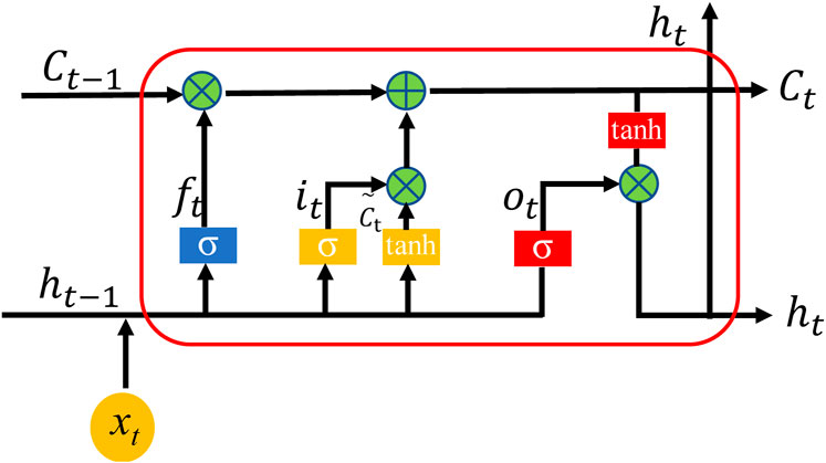
Figure 1. The structure of an LSTM network. f_t, i_t, and o_t are the information of the forget gate, input gate, and output gate, respectively. The terms σ and tanh respectively denote a sigmoid and a hyperbolic tangent activation function.

The forget gate controls the retention of information from the previous time step and the current time step by the sigmoid function and the forget gate can be expressed as Eq. 1:

$f_t=\sigma \left(W_f\left[h_{t-1},x_t\right]+b_f\right),(1)$

where W_f is the weight coefficient matrix of the forget gate layer, b_f is the bias term of the forget gate layer, h_t-1 is the result of the previous time step, x_t is the input value of the current time step, and f_t is the forget gate at the current time t.

The input gate is composed of two parts, the first part is to access the data saved to the memory cell at the current time step by the sigmoid function, and the second part is to generate new information to be stored in the memory cell by the tanh function, which can be expressed as Eqs 2, 3:

$i_t=\sigma \left(W_i\left[h_{t-1},x_t\right]+b_i\right),(2)$

${\stackrel{\sim }{C}}_t=\tanh \left(W_C\left[h_{t-1},x_t\right]+b_C\right),(3)$

where i_t is the input gate, σ is the sigmoid function, and tanh is the hyperbolic tangent activation function. W_i and b_i are the weight coefficient matrix and the bias term of the input gate, respectively, and ${\stackrel{\sim }{C}}_t$ is the current cell unit state of the input layer.

The memory value of the current time step is obtained by forgetting the information of the previous time step and inputting the information of the current time step, which can be expressed as Eq. 4:

$C_t=f_t\odot C_{t-1}+i_t\odot {\stackrel{\sim }{C}}_t,(4)$

where ⊙ is the Hadamard product.

The output gate controls the output of information, the output gate can be expressed as Eq. 5:

$o_t=\sigma \left(W_o\left[h_{t-1},x_t\right]+b_o\right),(5)$

where W_o represents the weight matrix of the output gate and b_o represents the bias term of the output gate.

The output result of the current time step can be expressed as Eq. 6:

$h_{tf}=o_t\odot \tanh \left(C_t\right),(6)$

The backward LSTM network is the reverse of the forward LSTM network, and the equation for each gate of the backward LSTM network is calculated as follows (Eqs 7–12):

$f_t=\sigma \left(W_f\left[h_{t+1},x_t\right]+b_f\right),(7)$

$i_t=\sigma \left(W_i\left[h_{t+1},x_t\right]+b_i\right),(8)$

${\stackrel{\sim }{C}}_t=\tanh \left(W_C\left[h_{t+1},x_t\right]+b_C\right),(9)$

$C_t=f_t\odot C_{t+1}+i_t\odot {\stackrel{\sim }{C}}_t,(10)$

$o_t=\sigma \left(W_o\left[h_{t+1},x_t\right]+b_o\right),(11)$

$h_{tb}=o_t\odot \tanh \left(C_t\right),(12)$

The forward LSTM network and the backward LSTM network only consider the impact of the previous time step or the next time step on the prediction results. The bidirectional LSTM network consists of a forward LSTM layer and a backward LSTM layer to learn the rules present in the data in both the forward and backward directions simultaneously. Figure 2 shows the structure of the bidirectional LSTM network.

Figure 2

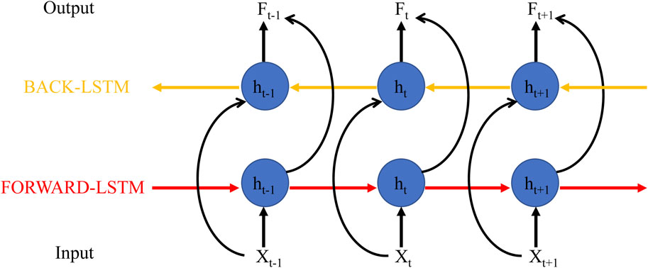
Figure 2. The structure of the bidirectional LSTM network.

The output of the bidirectional LSTM network at time step t can be expressed as follows (Eq. 13):

$F_t=W_{hf}{h}_{tf}+W_{hb}{h}_{tb}+b_h,(13)$

where h_tf and h_tb are the outputs of the forward LSTM layer and the backward LSTM layer at time step t. W_hf and W_hb are the corresponding weight parameters, respectively, and b_h is the bias parameter.

2.2 Attention mechanism

The principle of the attention mechanism is that in a large amount of information, limited attention resources are focused on a few key pieces of information that demand attention, useless and irrelevant information is ignored, and features are extracted for more critical and important information. With the introduction of an attention mechanism, the neural network can automatically learn and selectively focus on the important information in the input features, improving the model’s performance and generalization.

Figure 3 shows the attention mechanism. The features extracted from the LSTM layer are used as the input of the attention layer, and the expression is as follows (Vaswani et al., 2017, Eqs 14–16):

$e_i=\tanh \left(W{F}_i+b\right),(14)$

$a_i=\frac{\exp \left(e_i\right)}{{\displaystyle \sum _{j=1}^n}\exp \left(e_j\right)},(15)$

$D_i=a_i{F}_i,(16)$

where F_i is the output feature of the bidirectional LSTM layer, e_i is the attention distribution parameter for different features, and then e_i is normalized to obtain the weight parameter a_i for each feature, and D_i is the output of the attention mechanism layer, which is the input feature of the fully connected layer.

Figure 3

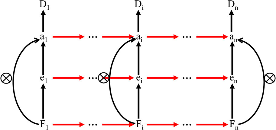
Figure 3. Schematic diagram of attentional mechanism.

2.3 1DCNN-BiLSTM-attention network

As shown in Figure 4, the 1DCNN-BiLSTM-Attention network proposed in this study first extracts the short-term features of the logging curves using the 1DCNN layer with the ReLU function, and the output is as follows (Eq. 17):

$C=\text{ReLU}\left(W_{\mathrm{c}}*X+b_c\right),(17)$

where $\text{ReLU}\left(x\right)=\max \left(x\right)$, W_c and b_c represent the weight matrix and bias, respectively, and * represents the convolution operation, X represents the input logging data.

Figure 4

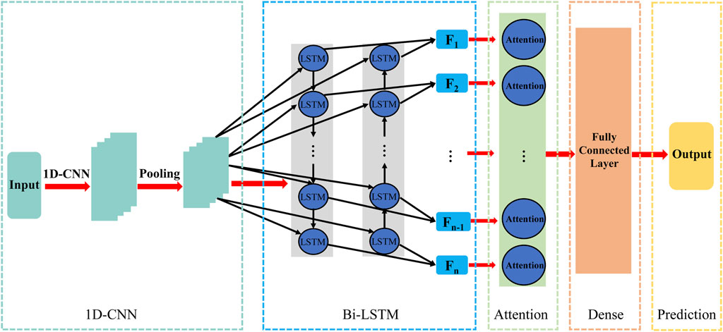
Figure 4. The structure of 1DCNN-BiLSTM-Attention network.

The convolution layer is followed by the pooling layer, which uses the maximum pooling method for feature down-sampling to decrease the dimension of the short-term feature data. Since the shallow and deep parts of the data of the logging curve are certainly connected, we feed the short-term features extracted by 1DCNN into the BiLSTM layer to further extract the long-term features. Then, the long-term features extracted by the Bi-LSTM layer are fed into the attention mechanism layer to reassign weights to obtain new features based on the importance of the features to the S-wave velocity, and finally, the new features are fed into the fully connected layer to establish the nonlinear relationship between the extracted features and the S-wave velocity.

3 Network building and training

3.1 Input feature selection

The selection of input features is a crucial step in building neural networks. In this study, we calculate the Pearson correlation coefficients to select the logging curves with high correlation with S-wave velocity as the input features of the 1DCNN-BiLSTM-Attention network. Using the logging data from four wells in the real field area, the Pearson correlation coefficients were calculated between the acoustic time difference curve (AC), compensated neutron curve (CNL), density curve (DEN), gamma curve (GR) and shear wave time difference curve (DTS). Figure 5 shows the heat analysis map of the four wells, it can be seen that, except for the density parameter, all the other three parameters are positively correlated with the DTS, and AC is the most strongly correlated with the DTS, in other words, the P-wave velocity plays the heaviest role in S-wave velocity prediction.

Figure 5

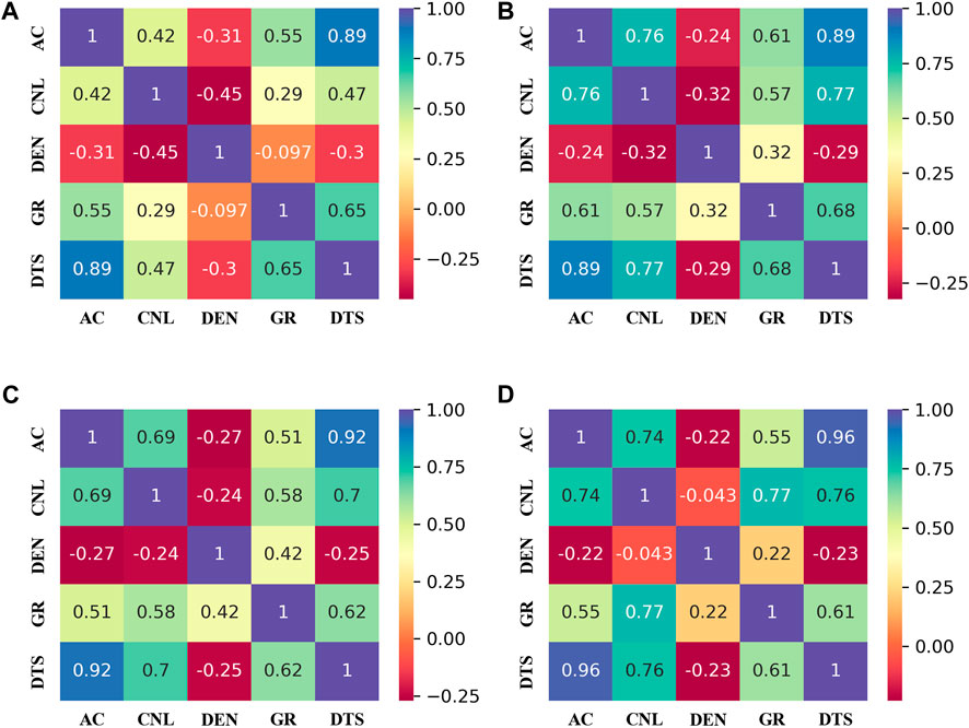
Figure 5. Correlation between the input logging curves and shear wave time difference curve (DTS): (A) Well A, (B) Well B, (C) Well C, and (D) Well D.

3.2 Input feature normalization

Input feature normalization has been widely used in machine learning and deep learning. Because the values of different logging curves are highly variable, if the data are not processed before network training, the training time will be long and the network may not converge to the minimum value, which limits the accuracy of the prediction model. Therefore, in this study, the min-max method is used to scale the logging data to the range [0-1] to eliminate these effects, and the expression is as follows (Eq. 18):

$X_{norm}=\frac{X-X_{\mathit{min}}}{X_{\mathit{max}}-X_{\mathit{min}}},(18)$

where X_norm is the normalized value, X is the original logging data, X_max is the maximum value of the logging data, and X_min is the minimum value of the logging data.

3.3 Network evaluation approach

The determination coefficient (R²), root mean square error (RMSE) function, and mean absolute error (MAE) function were utilized to evaluate the prediction performance of the method proposed in this study and the conventional S-wave velocity prediction method with the following expressions (Eqs 19–21):

$RMSE=\sqrt{\frac{1}{N}{\displaystyle \sum _{i=1}^N}{\left(y_i-p_i\right)}^2},(19)$

$MAE=\frac{1}{N}{\displaystyle \sum _{i=1}^N}\left|y_i-p_i\right|,(20)$

$R^2=1-\frac{{\displaystyle \sum _{i=1}^n}{\left(y_i-p_i\right)}^2}{{\displaystyle \sum _{i=1}^n}{\left(y_i-\overline{y}\right)}^2},(21)$

where N is the number of test sets, $y_i$ is the true value, p_i is the predicted value, and $\overline{y}$ is the average value of the real S-wave velocity.

4 Applications and results

We conducted two experiments to test the 1DCNN-BiLSTM-Attention network using data from four wells in a real field area. The first experiment is for the same well. We trained the prediction model using part of the data from Well A, and then the remaining data from Well A was tested. The second experiment is for the different wells. We trained the neural network using data from wells A and B, and then applied the trained network to wells C and D. To evaluate the accuracy of the model, we compared the prediction results of this model with those of conventional methods such as the LSTM network, BPNN, and empirical formula.

4.1 Comparison of the same well

The first experiment is a comparison of different S-wave velocity prediction methods in the same well. The logging data of Well A ranges from 1,452 to 2835.5 m with a sampling interval of 0.125 m and There are 11070 valid data after removing anomalous values. We utilize data in the depth range 1,452–2559 m for neural training, and data at depths ranging from 2,559 to 2835.5 m as a test set to test the prediction performance of the network. The network hyperparameters are set using the idea of the control variable method, the time step, the number of neurons in the LSTM layer, the number of convolution kernels, and the learning rate are regarded as variables, and only one of them is varied at a time, while the other parameters are kept unchanged, and the hyperparameter combination with the best prediction performance is selected. In this study, the hyperparameters are set as follows: the time step is 4, the number of LSTM neurons and convolution kernels is 32, the kernel size is set to 4*4, and the learning rate is 0.005. The loss function is chosen to be the mean squared error function (MSE), and the Adam optimization algorithm is used to make the network converge quickly. Additionally, to avoid the overfitting problem of the network during the training process, a dropout layer is added after both the pooling layer and the bidirectional LSTM layer, and the discard rate of the dropout layer is set to 0.4, which means that 40% of the neurons are deactivated each time, which is more helpful for the convergence of the network.

The logging data after preprocessing is fed into the neural network for training, as shown in Figure 6, the loss value of the network reaches a smaller value after 40 epochs, and after 45 epochs, the training loss value and the validation loss value are equal and no longer change indicating that the network has converged to a minimum and could be applied to the shear wave velocity prediction.

Figure 6

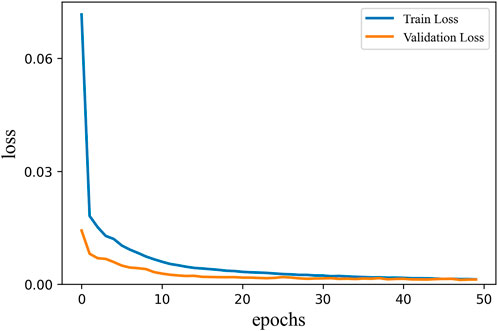
Figure 6. Training process of the 1DCNN-BiLSTM-Attention network (blue line: train loss, orange line: validation loss).

Similarly, the LSTM network and BP neural network are trained using the same dataset. The hyperparameters of the LSTM network are set as follows: the time step is 4, the number of LSTM layers is 5, and the learning rate is 0.005. The loss function is chosen to be the mean squared error function (MSE), and the Adam optimization algorithm is used to make the network converge quickly. The number of fully connected layers of the BPNN is 4. The learning rate, loss function, and optimization algorithm are the same as those of the LSTM network. Figure 7 shows the training loss errors of the 1DCNN-BiLSTM-Attention network, the LSTM network, and BPNN. It can be seen that after 45 epochs all the networks have converged, and the 1DCNN-BiLSTM-Attention network has the lowest loss error, followed by the LSTM network, and the BPNN has the highest loss value. The empirical formula (Han et al., 1986, Eq. 22) for comparison with the method proposed in this study can be expressed as follows:

$V_s=0.794V_p-0.787,(22)$

where V_p and V_s are the P-wave velocity and S-wave velocity, km/s.

Figure 7

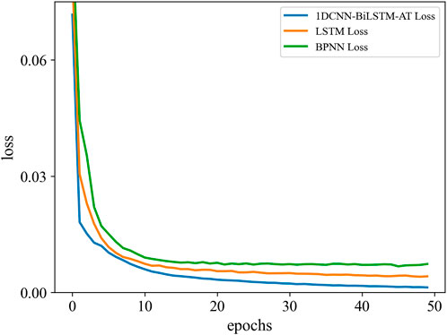
Figure 7. Loss error curves of 1DCNN-BiLSTM-Attention network, LSTM network, and BPNN (blue line: 1DCNN-BiLSTM-Attention network train loss, orange line: LSTM network train loss, green line: BPNN train loss).

Figure 8 shows the prediction results of the four prediction methods on the test set of Well A compared with the real values. The left side of Figure 8 shows the four logging curves of Well A, the logging data in the red box is the test set, and the logging data outside the red box is the training set. The black line on the right side of Figure 8 shows the real logging S-wave velocity, and the other colors are the prediction results of the corresponding methods, respectively. From the figure, we can find that the prediction results of the method proposed in this study are closer to the real logging S-wave velocity than the other three shear wave velocity prediction methods, both in terms of prediction value and velocity tendency. At the purple arrows (2,640–2680, 2,738–2742 m), those are the areas where the S-wave velocity changes are more vigorously, and for this case, the 1DCNN-BiLSTM-Attention network achieves the best prediction results, which indicates that the method can simultaneously explore the connection and pattern of the logging curves in the depth, highlight the features that have a greater impact on the S-wave velocity, and then get more accurate prediction results. Figure 9 shows the cross-plot of S-wave velocity prediction results using four methods. It is very apparent that the S-wave velocity predicted by the 1DCNN-BiLSTM-Attention network is more consistent with the real S-wave velocity, and the S-wave velocity predicted by the empirical formula is more dispersed and incorrect.

Figure 8

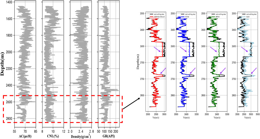
Figure 8. Prediction results for Well A (black line: Real value, red line: 1DCNN-BiLSTM-Attention network, blue line: LSTM network, green line: BPNN, and light blue line: Empirical formula).

Figure 9

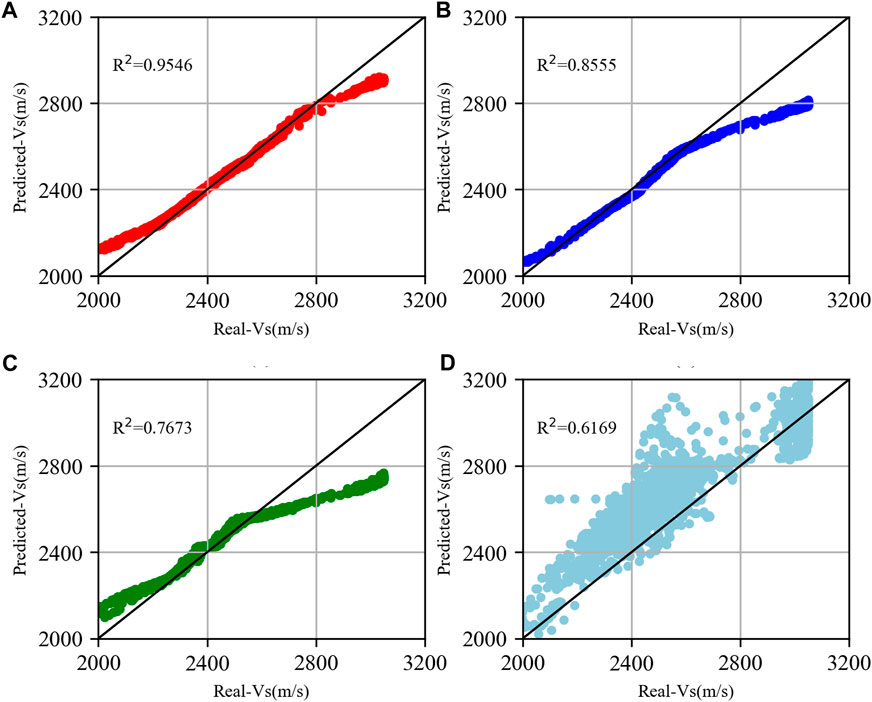
Figure 9. Prediction results for Well A. (A) 1DCNN-BiLSTM-Attention network, (B) LSTM network, (C) BPNN, and (D) Empirical formula. The R² show the prediction accuracy for all methods.

We analyze the errors of the prediction results to compare the prediction performance of the different methods. Figure 10 shows the error histograms of the four methods, and it can be clearly seen from Figure 8A that the prediction errors of the 1DCNN-BiLSTM-Attention network are all concentrated around error=0, with a more uniform distributed, which exhibits an excellent prediction performance and can be generalized to other logging data for S-wave prediction. The prediction errors of the other three benchmark methods have a wider range, and the prediction error of Han’s empirical formula is concentrated around 250 m/s, which is unacceptable and shows the empirical formula’s limitations in the real field.

Figure 10

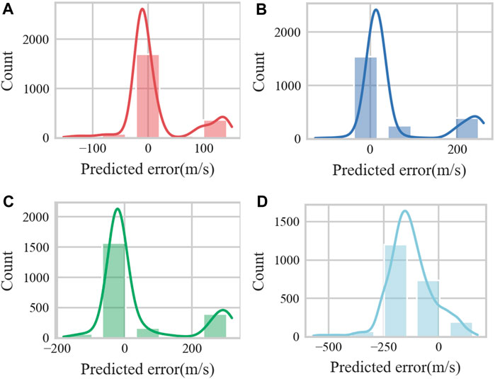
Figure 10. The error histograms for the four methods of Well A: (A) 1DCNN-BiLSTM-Attention network, (B) LSTM network, (C) BPNN, and (D) Empirical formula.

We employed determination coefficient (R²), MAE, and RMSE to evaluate the performance of different models. Table 1 shows the R², MAE, and RMSE of Well A. The R², MAE, and RMSE of the LSTM network are 0.9546, 34.68, and 56.29 m/s, respectively, obtaining the highest R² and the lowest MAE and RMSE among all models. Compared with the LSTM network, BPNN, and empirical formula, the prediction accuracy of the 1DCNN-BiLSTM-Attention network increased by 11.58%, 24.41%, and 54.74%, respectively; the MAE reduced by 37.86%, 54.48%, and 75.56%, respectively; and the RMSE reduced by 43.96%, 55.84%, and 84.14%, respectively. It is clear that the 1DCNN-BiLSTM-Attention network can simultaneously explore the connection and pattern of the logging curves in-depth, highlight the features that have a greater impact on the S-wave velocity, and then get more accurate prediction results.

Table 1

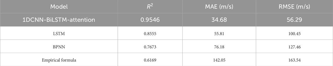
Table 1. Comparison of Well A prediction results.

4.2 Comparison of the different wells

The second experiment is a comparison of different S-wave velocity prediction methods in different wells. 25755 sets of data from wells A and B of a real field area are employed as the training set of the neural network, and 4,103 sets of data from wells C (1957–2250 m) and D (1948–2220 m) are utilized as the test set to verify the prediction performance and generalization of the network. Similarly, the prediction results of the proposed method in the study were compared with those of other three methods. The input features and network hyperparameters for this experiment remain unchanged from the previous section, i.e., AC, CNL, DEN, and GR. Figures 11, 12 show the results of the four methods and the comparison between the predicted and measured values of S-wave velocity in wells C and D, respectively, in which the black curves are the real logging S-wave velocity values, and the other colors are the prediction results of the corresponding methods. From the two figures, it can be seen that the four methods show a certain prediction effect on the S-wave velocity of the two wells, and the trend of the prediction results is also consistent with the trend of the real S-wave logging velocity. However, it is obvious that the prediction results of the 1DCNN-BiLSTM-Attention network are closer to the real measurements, and the prediction performance of the empirical formula is significantly poor compared to the other three methods.

Figure 11

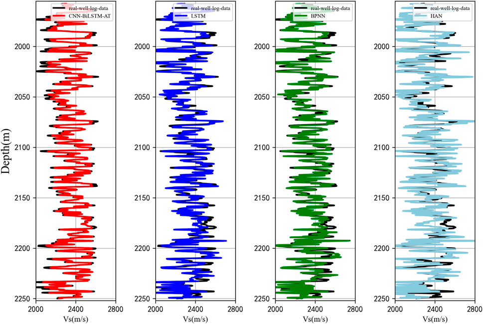
Figure 11. Prediction results for Well C (black line: Real value, red line: 1DCNN-BiLSTM-Attention network, blue line: LSTM network, green line: BPNN, and light blue line: Empirical formula).

Figure 12

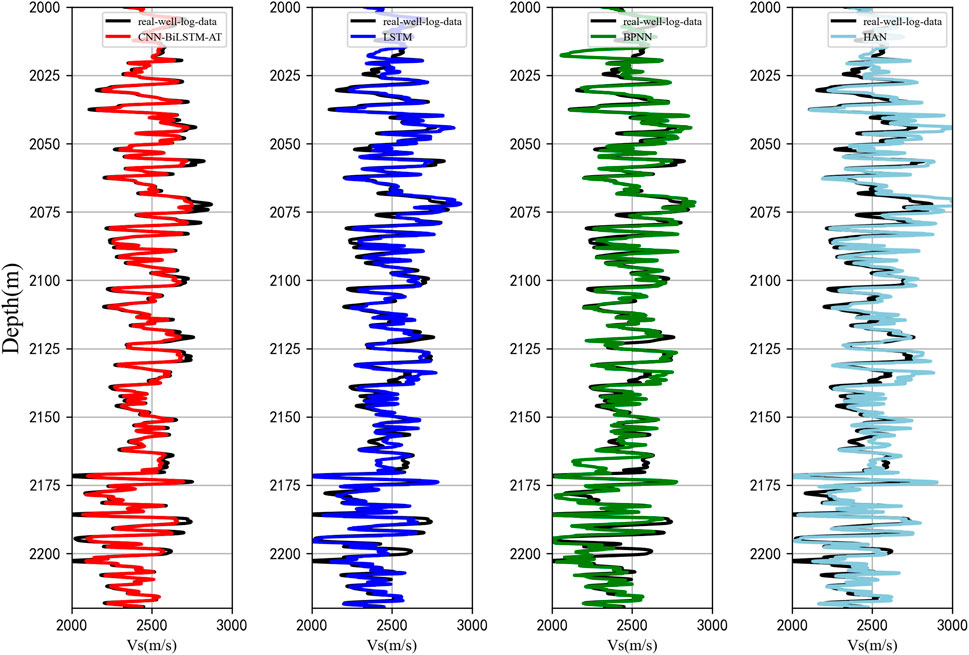
Figure 12. Prediction results for Well D (black line: Real value, red line: 1DCNN-BiLSTM-Attention network, blue line: LSTM network, green line: BPNN, and light blue line: Empirical formula).

Figure 13 shows the cross-plot of the true S-wave velocity values and the predicted S-wave velocity values using the four methods. It is obvious that the S-wave velocity prediction using the method proposed in this study and real S-wave velocity is consistent with the slope in Figure 13, and the cross-plots of the predicted results of the other three methods are away from the line y=x. Furthermore, the R² was 0.9752 and 0.9680, respectively, much greater than the other three methods, indicating that our proposed method has better prediction performance. For Well C, the prediction accuracy of the 1DCNN-BiLSTM-Attention network increased by 17.99%, 22.60%, and 81.89%, respectively, compared to the other three methods, and for Well D, the prediction accuracy of the 1DCNN-BiLSTM-Attention network increased by 18.53%, 34.15%, and 30.35%, respectively.

Figure 13

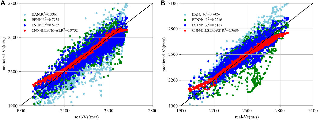
Figure 13. Cross-plot of predicted results and real measured values: (A) Well C, (B) Well D.

Figure 14 shows the absolute value curve of the relative error of the prediction results of the two wells using different methods. As can be seen from the figure, the prediction error of the method proposed in this study is basically below 4% for Well C and below 3% for Well D, which is lower than the other three methods.

Figure 14

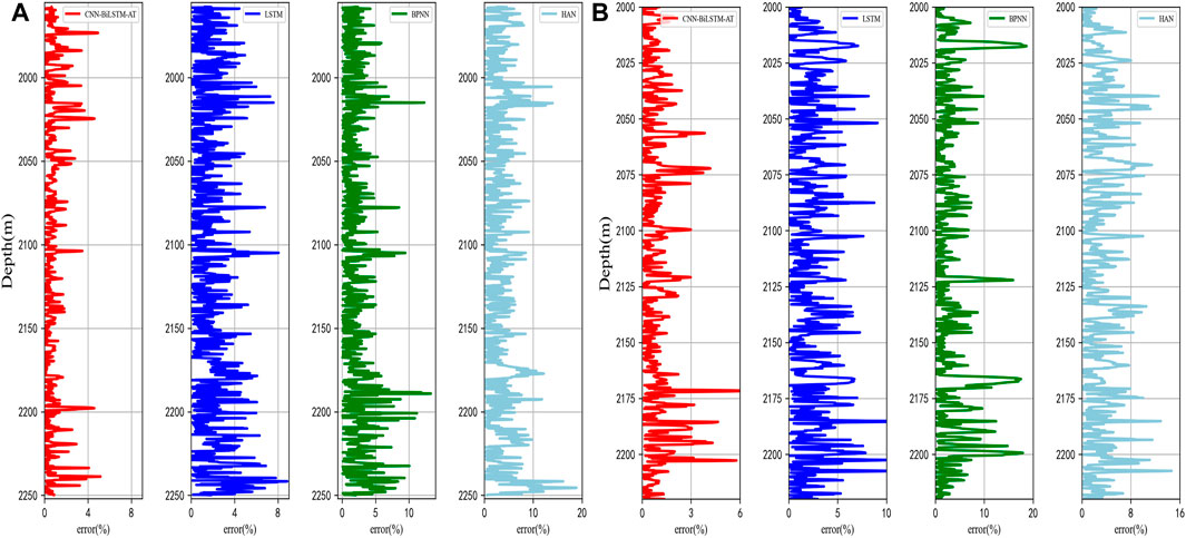
Figure 14. Relative errors of prediction results: (A) Well C, (B) Well D.

Tables 2, 3 show the R², MAE, and RMSE of the prediction results of the four methods. The 1DCNN-BiLSTM-Attention network has the highest R² compared with the benchmark methods, indicating that the 1DCNN-BiLSTM-Attention network has the best prediction accuracy. The MAE and RMSE of the prediction results of wells C and D using the approach proposed in this study are smaller than those of the LSTM network, BPNN, and empirical formula, demonstrating excellent prediction performances and prediction accuracy, and the 1DCNN-BiLSTM-Attention network trained using wells A and B can be well generalized and applied to wells C and D, exhibiting excellent generalization of the network.

Table 2

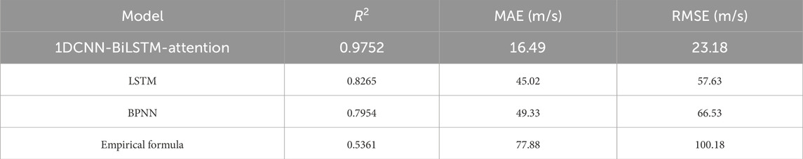
Table 2. Sampling range of tight sandstone model parameters.

Table 3

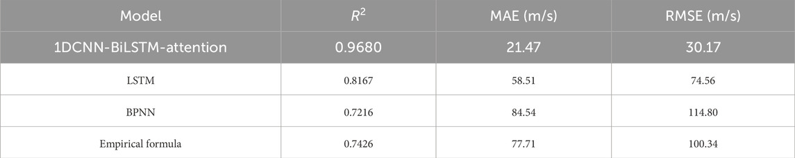
Table 3. petrophysical parameters of five tight sandstone samples.

5 Discussion

In this paper, we propose a new deep learning framework for S-wave velocity prediction, under which we build a new network including 1DCNN, BiLSTM network, and fully connected neural network, which combines the advantages of CNN and LSTM network in feature extraction and introduces the attention mechanism. However, it is clear that the network is ultimately still a supervised learning network, and its powerful prediction ability depends on sufficient high-quality labeled data. The requirement for accurate labels often forces us to use synthetic data to train our network because the labels in synthetic data are readily available (Wu et al., 2019; Yang and Ma, 2019). However, synthetic data often fail to describe the real conditions in the field area, which ultimately leads to poor generalization of the well-trained neural network. Therefore, reducing the difference between synthetic and real data, as well as making the distribution of synthetic data similar to that of real data, is an interesting method for improving the generalizability of networks (Alkhalifah et al., 2022; Zhang et al., 2022). Meanwhile, how to establish mapping relationships for small sample datasets is what we need to explore in the future, and how to improve the generalization ability of the network as well as enhance the prediction performance of networks through small sample datasets is also what we need to consider.

6 Summary and conclusion

S-wave velocity estimation is an important task in reservoir prediction. Considering the patterns and connections of logging data in depth and the limitations of traditional LSTM networks and CNNs for sequence data prediction, this study proposes a new neural network, the 1DCNN-BiLSTM-Attention network, for logging S-wave velocity prediction. This network combines the strengths of CNN and RNN for feature extraction. We first extract the local features of logging curves using 1DCNN, then extract the long-term sequence features of logging curves using the BiLSTM network, and at the same time add an attention layer following the BiLSTM network to further highlight the features that are more important for S-wave velocity prediction. The well-trained network is applied to the real field data, including the same well and different well applications, and the four input logging data (AC, CNL, DEN, and GR) as input features. The prediction accuracies of the three wells are 0.9546, 0.9752, and 0.9680, respectively, with RMSE less than 57 m/s and MAE less than 35 m/s. Using the same test logging data, the LSTM network achieves S-wave velocity prediction accuracy of R²<0.86, RMSE>57 m/s, MAE>45 m/s, the BPNN achieves S-wave velocity prediction accuracy of R²<0.80, RMSE>66 m/s, MAE>49 m/s, and Han’s empirical formula achieves S-wave velocity prediction accuracy of R²<0.75, RMSE>100 m/s, MAE>77 m/s. Obviously, compared with the three traditional S-wave velocity prediction methods, the proposed new network exhibits better prediction performance and generalization ability and can provide accurate S-wave velocity parameters for reservoir prediction. However, it cannot be ignored that the 1DCNN-BiLSTM-Attention network proposed in this study is a supervised learning algorithm, and its prediction accuracy depends on the quality and quantity of labels. Therefore, we need to consider how to improve the generalization and robustness of the neural network.

Data availability statement

The raw data supporting the conclusion of this article will be made available by the authors, without undue reservation.

Author contributions

GF: Writing–original draft, Writing–review and editing. W-QL: Validation, Writing–review and editing. ZY: Supervision, Writing–review and editing. WY: Data curation, Writing–review and editing.

Funding

The author(s) declare that financial support was received for the research, authorship, and/or publication of this article. This work is sponsored by the CNPC (China National Petroleum Corporation) Scientific Research and Technology Development Project (Grant No. 2021DJ05) and the Research on Geophysical Description Technology of Continental Clastic Reservoir and Field Test (2022KT1505).

Conflict of interest

GF, W-QL, ZY and WY was employed by PetroChina.

Publisher’s note

All claims expressed in this article are solely those of the authors and do not necessarily represent those of their affiliated organizations, or those of the publisher, the editors and the reviewers. Any product that may be evaluated in this article, or claim that may be made by its manufacturer, is not guaranteed or endorsed by the publisher.

Abbreviations

1DCNN, One-dimensional convolutional neural network; AC, Acoustic time difference; ANN, Artificial neural network; BiLSTM, Bidirectional long short-term memory; BPNN, Back propagation neural network; CNL, Compensated neutron; DEN, Density; DL, Deep learning; DT, Compressional wave slowness (delta T); DTS, Shear wave time difference; GR, Gamma ray; GRU, Gated Recurrent Unit; LSTM, Long short-term memory; MAE, Mean absolute error; ML, Machine learning; MSE, Mean squared error; RNNs, Recurrent neural networks; R², Determination coefficient; RMSE, Root mean square error; S-wave, Shear wave; V_P, Compressional-wave velocity.

References

Abad, A. R. B., Tehrani, P. S., Naveshki, M., Ghorbani, H., Mohamadian, N., Davoodi, S., et al. (2021). Predicting oil flow rate through orifice plate with robust machine learning algorithms. Flow Meas. Instrum. 81, 102047. doi:10.1016/j.flowmeasinst.2021.102047

CrossRef Full Text | Google Scholar

Ali, M., Ma, H., Pan, H., Ashraf, U., and Jiang, R. (2020). Building a rock physics model for the formation evaluation of the lower goru sand reservoir of the southern indus basin in Pakistan. J. Petroleum Sci. Eng. 194, 107461. doi:10.1016/j.petrol.2020.107461

CrossRef Full Text | Google Scholar

Alimoradi, A., Shahsavani, H., and Rouhani, A. K. (2011). Prediction of shear wave velocity in underground layers using SASW and artificial neural networks. Engineering 03, 266–275. doi:10.4236/eng.2011.33031

CrossRef Full Text | Google Scholar

Alkhalifah, T., Wang, H., and Ovcharenko, O. (2022). MLReal: bridging the gap between training on synthetic data and real data applications in machine learning. Artif. Intell. Geosciences 3, 101–114. doi:10.1016/j.aiig.2022.09.002

CrossRef Full Text | Google Scholar

Assefa, S., McCann, C., and Sothcott, J. (2003). Velocities of compressional and shear waves in limestones. Geophys. Prospect. 51, 1–13. doi:10.1046/j.1365-2478.2003.00349.x

CrossRef Full Text | Google Scholar

Azadpour, M., Saberi, M. R., Javaherian, A., and Shabani, M. (2020). Rock physics model-based prediction of shear wave velocity utilizing machine learning technique for a carbonate reservoir, southwest Iran. J. Petroleum Sci. Eng. 195, 107864. doi:10.1016/j.petrol.2020.107864

CrossRef Full Text | Google Scholar

Bagheripour, P., Gholami, A., Asoodeh, M., and Vaezzadeh-Asadi, M. (2015). Support vector regression based determination of shear wave velocity. J. Petroleum Sci. Eng. 125, 95–99. doi:10.1016/j.petrol.2014.11.025

CrossRef Full Text | Google Scholar

Bengio, Y., Simard, P., and Frasconi, P. (1994). Learning long-term dependencies with gradient descent is difficult. IEEE Trans. Neural Netw. 5, 157–166. doi:10.1109/72.279181

PubMed Abstract | CrossRef Full Text | Google Scholar

Biot, M. A. (1956a). Theory of propagation of elastic waves in a fluid-saturated porous Solid. I. Low-Frequency range. J. Acoust. Soc. Am. 28, 168–178. doi:10.1121/1.1908239

CrossRef Full Text | Google Scholar

Biot, M. A. (1956b). Theory of propagation of elastic waves in a fluid-saturated porous Solid. II. Higher frequency range. J. Acoust. Soc. Am. 28, 179–191. doi:10.1121/1.1908241

CrossRef Full Text | Google Scholar

Castagna, J. P., Batzle, M. L., and Eastwood, R. L. (1985). Relationships between compressional-wave and shear-wave velocities in clastic silicate rocks. GEOPHYSICS 50, 571–581. doi:10.1190/1.1441933

CrossRef Full Text | Google Scholar

Chen, T., Gao, G., Wang, P., Zhao, B., Li, Y., and Gui, Z. (2022). Prediction of shear wave velocity based on a hybrid network of two-dimensional convolutional neural network and gated recurrent unit. Geofluids 2022, 1–14. doi:10.1155/2022/9974157

CrossRef Full Text | Google Scholar

Chen, W., Yang, L., Bei, Z., Zhang, M., and Chen, Y. (2020). Deep learning reservoir porosity prediction based on multilayer long short-term memory network. GEOPHYSICS 85, WA213–WA225. doi:10.1190/geo2019-0261.1

CrossRef Full Text | Google Scholar

Chen, Y., Saad, O. M., Savvaidis, A., Chen, Y., and Fomel, S. (2022). 3D micro-seismic monitoring using machine learning. J. Geophys. Res. Solid Earth 127, e2021JB023842. doi:10.1029/2021JB023842

CrossRef Full Text | Google Scholar

Ewees, A. A., Thanh, H. V., Al-qaness, M. A. A., Abd Elaziz, M., and Samak, A. H. (2024). Smart predictive viscosity mixing of CO2–N2 using optimized dendritic neural networks to implicate for carbon capture utilization and storage. J. Environ. Chem. Eng. 12, 112210. doi:10.1016/j.jece.2024.112210

CrossRef Full Text | Google Scholar

Feng, G., Zeng, H., Xu, X., Tang, G., and Wang, Y. (2023). Shear wave velocity prediction based on deep neural network and theoretical rock physics modeling. Front. Earth Sci. 10. doi:10.3389/feart.2022.1025635

CrossRef Full Text | Google Scholar

Gassmann, F. (1951). Elastic waves through a packing of spheres. GEOPHYSICS 16, 673–685. doi:10.1190/1.1437718

CrossRef Full Text | Google Scholar

Greenberg, M. L., and Castagna, J. P. (1992). Shear-wave velocity estimation in porous rocks: theoretical formulation, preliminary verification and applications. Geophys. Prospect. 40, 195–209. doi:10.1111/j.1365-2478.1992.tb00371.x

CrossRef Full Text | Google Scholar

Han, D., Nur, A., and Morgan, D. (1986). Effects of porosity and clay content on wave velocities in sandstones. GEOPHYSICS 51, 2093–2107. doi:10.1190/1.1442062

CrossRef Full Text | Google Scholar

Harsuko, R., and Alkhalifah, T. A. (2022). StorSeismic: a new paradigm in deep learning for seismic processing. IEEE Trans. Geoscience Remote Sens. 60: 1–15. doi:10.1109/TGRS.2022.3216660

CrossRef Full Text | Google Scholar

Jiang, R., Ji, Z., Mo, W., Wang, S., Zhang, M., Yin, W., et al. (2022). A novel method of deep learning for shear velocity prediction in a tight sandstone reservoir. Energies 15, 7016. doi:10.3390/en15197016

CrossRef Full Text | Google Scholar

Lee, M. W. (2006). A simple method of predicting S-wave velocity. GEOPHYSICS 71, F161–F164. doi:10.1190/1.2357833

CrossRef Full Text | Google Scholar

Li, Q. J. (1992). Velocity regularities of P and S-waves in formations. Oil Geophys. Prospect. 27, 1–12. doi:10.13810/j.cnki.issn.1000-7210.1992.01.001

CrossRef Full Text | Google Scholar

Liu, J., Gui, Z., Gao, G., Li, Y., Wei, Q., and Liu, Y. (2023). Predicting shear wave velocity using a convolutional neural network and dual-constraint calculation for anisotropic parameters incorporating compressional and shear wave velocities. Processes 11 (8), 2356. doi:10.3390/pr11082356

CrossRef Full Text | Google Scholar

Maleki, S., Moradzadeh, A., Reza, G. R., Gholami, R., and Sadeghzadeh, F. (2014). Prediction of shear wave velocity using empirical correlations and artificial intelligence methods. NRIAG J. Astronomy Geophys. 3, 70–81. doi:10.1016/j.nrjag.2014.05.001

CrossRef Full Text | Google Scholar

Mehrgini, B., Izadi, H., and Memarian, H. (2017). Shear wave velocity prediction using elman artificial neural network. Carbonates Evaporites 34, 1281–1291. doi:10.1007/s13146-017-0406-x

CrossRef Full Text | Google Scholar

Mousavi, S. M., Langston, C. A., and Horton, S. P. (2016). Automatic micro-seismic denoising and onset detection using the synchrosqueezed continuous wavelet transform. Geophysics 81 (4), V341–V355. doi:10.1190/geo2015-0598.1

CrossRef Full Text | Google Scholar

Oh, J. W., Kalita, M., and Alkhalifah, T. (2018). 3D elastic full-waveform inversion using P-wave excitation amplitude: application to ocean bottom cable field data. Geophysics 83, R129–R140. doi:10.1190/geo2017-0236.1

CrossRef Full Text | Google Scholar

Oloruntobi, O., and Butt, S. (2020). The shear-wave velocity prediction for sedimentary rocks. J. Nat. Gas Sci. Eng. 76, 103084. doi:10.1016/j.jngse.2019.103084

CrossRef Full Text | Google Scholar

Pickett, G. R. (1963). Acoustic character logs and their applications in formation evaluation. J. Petroleum Technol. 15, 659–667. doi:10.2118/452-pa

CrossRef Full Text | Google Scholar

Pride, S. R., Berryman, J. G., and Harris, J. M. (2004). Seismic attenuation due to wave-induced flow. J. Geophys. Res. Solid Earth 109, 247–278. doi:10.1029/2003JB002639

CrossRef Full Text | Google Scholar

Rajabi, M., Omid, H., Davoodi, S., Wood, D. A., Pezhman, S. T., Ghorbani, H., et al. (2022). Predicting shear wave velocity from conventional well logs with deep and hybrid machine learning algorithms. J. Petroleum Explor. Prod. Technol. 13, 19–42. doi:10.1007/s13202-022-01531-z

CrossRef Full Text | Google Scholar

Rezaee, M. R., Ilkhchi, A. K., and Barabadi, A. (2007). Prediction of shear wave velocity from petrophysical data utilizing intelligent systems: an example from a sandstone reservoir of carnarvon basin, Australia. J. Petroleum Sci. Eng. 55, 201–212. doi:10.1016/j.petrol.2006.08.008

CrossRef Full Text | Google Scholar

Russell, B. H., Hedlin, K., Hilterman, F. J., and Lines, L. R. (2003). Fluid-property discrimination with avo: a biot-gassmann perspective. GEOPHYSICS 68, 29–39. doi:10.1190/1.1543192

CrossRef Full Text | Google Scholar

Saad, O. M., Huang, G., Chen, Y., Savvaidis, A., Fomel, S., Pham, N., et al. (2021). SCALODEEP: a highly generalized deep learning framework for real-time earthquake detection. J. Geophys. Res. Solid Earth 126, e2020JB021473. doi:10.1029/2020JB021473

CrossRef Full Text | Google Scholar

Staudemeyer, R. C., and Morris, E. R. (2019). Understanding LSTM -- a tutorial into long short-term memory recurrent neural networks. arXiv (Cornell Univ.) 1909, 09586. doi:10.48550/arxiv.1909.09586

CrossRef Full Text | Google Scholar

Sun, Y., and Liu, Y. (2020). Prediction of S-wave velocity based on GRU neural network. Oil Geophys. Prospect. 55, 484–492. doi:10.13810/j.cnki.issn.1000-7210.2020.03.001

CrossRef Full Text | Google Scholar

Thanh, H. V., Dai, Z., Du, Z., Yin, H., Yan, B., Soltanian, M. R., et al. (2024b). Artificial intelligence-based prediction of hydrogen adsorption in various kerogen types: implications for underground hydrogen storage and cleaner production. Int. J. Hydrogen Energy 57, 1000–1009. doi:10.1016/j.ijhydene.2024.01.115

CrossRef Full Text | Google Scholar

Thanh, H. V., Zhang, H., Dai, Z., Zhang, T., Tangparitkul, S., and Min, B. (2024a). Data-driven machine learning models for the prediction of hydrogen solubility in aqueous systems of varying salinity: implications for underground hydrogen storage. Int. J. Hydrogen Energy 55, 1422–1433. doi:10.1016/j.ijhydene.2023.12.131

CrossRef Full Text | Google Scholar

Vaswani, A., Shazeer, N., Parmar, N., Uszkoreit, J., Jones, L., Gomez, A. N., et al. (2017). Attention is all you need. Proc. Adv. Neural Inf. Process. Syst. 30, 1–11. doi:10.48550/arXiv.1706.03762

CrossRef Full Text | Google Scholar

Wang, J., and Cao, J. (2021). Data-driven S-wave velocity prediction method via a deep-learning-based deep convolutional gated recurrent unit fusion network. GEOPHYSICS 86, M185–M196. doi:10.1190/geo2020-0886.1

CrossRef Full Text | Google Scholar

Wang, J., Cao, J., Zhao, S. G., and Qi, Q. (2022). S-wave velocity inversion and prediction using a deep hybrid neural network. Sci. China Earth Sci. 65, 724–741. doi:10.1007/s11430-021-9870-8

CrossRef Full Text | Google Scholar

Wang, P., and Peng, S. (2019). On a new method of estimating shear wave velocity from conventional well logs. J. Petroleum Sci. Eng. 180, 105–123. doi:10.1016/j.petrol.2019.05.033

CrossRef Full Text | Google Scholar

Wu, X., Geng, Z., Shi, Y., Pham, N., Fomel, S., and Caumon, G. (2019). Building realistic structure models to train convolutional neural networks for seismic structural interpretation. Geophysics 85 (4), WA27–WA39. doi:10.1190/geo2019-0375.1

CrossRef Full Text | Google Scholar

Xu, S., and Payne, M. A. (2009). Modeling elastic properties in carbonate rocks. Lead. Edge 28, 66–74. doi:10.1190/1.3064148

CrossRef Full Text | Google Scholar

Xu, S.-Y., and White, R. (1995). A new velocity model for clay-sand mixtures 1. Geophys. Prospect. 43, 91–118. doi:10.1111/j.1365-2478.1995.tb00126.x

CrossRef Full Text | Google Scholar

Xu, S.-Y., and White, R. (1996). A physical model for shear-wave velocity Prediction1. Geophys. Prospect. 44, 687–717. doi:10.1111/j.1365-2478.1996.tb00170.x

CrossRef Full Text | Google Scholar

Yang, F., and Ma, J. (2019). Deep-learning inversion: a next-generation seismic velocity model building method. Geophysics 84 (4), R583–R599. doi:10.1190/geo2018-0249.1

CrossRef Full Text | Google Scholar

Yang, L., Fomel, S., Wang, S., Chen, X., Chen, W., Saad, O. M., et al. (2023). Porosity and permeability prediction using a transformer and periodic long short-term network. Geophysics 88 (1), WA293–WA308. doi:10.1190/geo2022-0150.1

CrossRef Full Text | Google Scholar

Yin, X., and Li, L. (2015). P-wave and S-wave velocities inversion based on rock physics model. Geophys. Prospect. Petroleum 54, 249–253. doi:10.3969/j.issn.1000-1441.2015.03.001

CrossRef Full Text | Google Scholar

You, J., Cao, J., Wang, X., and Liu, W. (2021). Shear wave velocity prediction based on LSTM and its application for morphology identification and saturation inversion of gas hydrate. J. Petroleum Sci. Eng. 205, 109027. doi:10.1016/j.petrol.2021.109027

CrossRef Full Text | Google Scholar

Yuan, S., Liu, J., Wang, S., Wang, T., and Shi, P. (2018). Seismic waveform classification and first-break picking using convolution neural networks. IEEE Geoscience Remote Sens. Lett. 15 (2), 272–276. doi:10.1109/LGRS.2017.2785834

CrossRef Full Text | Google Scholar

Zhang, H., Alkhalifah, T., Liu, Y., Birnie, C., and Di, X. (2022). Improving the generalization of deep neural networks in seismic resolution enhancement. IEEE Geoscience Remote Sens. Lett. 20, 1–5. doi:10.1109/LGRS.2022.3229167

CrossRef Full Text | Google Scholar

Zhang, H., Wang, P., Rahimi, M., Vo Thanh, H., Wang, Y., Dai, Z., et al. (2024). Catalyzing net-zero carbon strategies: enhancing CO2 flux Prediction from underground coal fires using optimized machine learning models. J. Clean. Prod. 441, 141043. doi:10.1016/j.jclepro.2024.141043

CrossRef Full Text | Google Scholar

Zhang, Y., Zhang, C., Ma, Q., Zhang, X., and Zhou, H. (2021). Automatic prediction of shear wave velocity using convolutional neural networks for different reservoirs in ordos basin. J. Petroleum Sci. Eng. 208, 109252. doi:10.1016/j.petrol.2021.109252

CrossRef Full Text | Google Scholar

Zhang, Y., Zhong, H., Wu, Z., Zhou, H., and Ma, Q. (2020). Improvement of petrophysical workflow for shear wave velocity prediction based on machine learning methods for complex carbonate reservoirs. J. Petroleum Sci. Eng. 192, 107234. doi:10.1016/j.petrol.2020.107234

CrossRef Full Text | Google Scholar