Pre-stack seismic inversion based on model-constrained generative adversarial network

Pre-stack seismic inversion usually uses various traditional algorithms to estimate elastic parameters such as P-wave velocity, S-wave velocity, and density. It is hard to derive accurate elastic parameters due to their non-uniqueness and high dimensionality between elastic parameters and seismic data, the calculation of elastic parameters is inaccurate. Convolutional Neural Networks (CNNs) have high-dimensional feature space mapping capabilities, which are utilized to establish mapping relationships between seismic data and elasticity parameters. However, their effectiveness is greatly affected by label data, and at the same time, due to the lack of enough label data, resulting in a low degree of fitting between prediction results and real data. In addition, conventional seismic inversion methods based on CNNs lack physical model constraints, resulting in low accuracy and poor interpretability of prediction results. We propose a Cycle-consistent Generative Adversarial Network based on a geophysical mechanism (SeisInv-CycleGAN). Deterministic inversion results and labeled data are combined into hybrid geophysical data as a training set of SeisInv-CycleGAN with geophysical constraints. At the same time, the residual (seismic loss) between the seismic data synthesized by forward modeling and the actual data is used as part of the loss function. The SeisInv-CycleGAN does not require building an initial model, and it can achieve higher accuracy in prediction results with a small amount of labeled data.

1 Introduction

1.1 CycleGAN and loss function

Pre-stack seismic inversion, based on pre-stack seismic data and well-logging data, allows for the inversion of various elastic parameters, which can then be used to predict reservoir properties and hydrocarbon potential (Li et al., 2019). However, the geological conditions of reservoirs have become more complex, making it difficult to establish accurate relationships between seismic data and reservoir parameters. To solve this problem, artificial neural networks (ANN) have been applied in the inversion field (Zhao and Gui, 2005; Zhang H. et al., 2022; Liu et al., 2022; Zhou et al., 2022). ANN has been successfully employed in geophysics to determine non-linear relationships in data (Röth and Tarantola, 1994; Yin et al., 1994). Due to their simple structures and immature technology, ANNs were not widely used in geophysics. Recently, there has been a surge in academic interest in using deep learning to solve geophysical problems, with Yu and Ma (2021) analyzing the current and future situation of deep learning in geophysics, covering data processing, inversion, and interpretation.

Convolutional Neural Networks (CNN) and Recurrent Neural Networks (RNN) are most widely used in seismic inversion. Das et al. (2019) proposed a method based on one-dimensional CNN for seismic impedance inversion, demonstrating the great potential of CNN in predicting high-frequency impedance from low-frequency signals. Phan and Sen, (2018) introduced a pre-stack AVA waveform inversion method using Hopfield-based CNN (CHNN), inverting pre-stack angle gathers to angle reflection coefficients and then converting them to P-wave and S-wave velocities and density parameters. Wang J. et al. (2022) employed Residual Networks (ResNet) and causal convolution to build a Time Domain Convolutional Neural Network (TCN), establishing a mapping relationship between seismic data and wave impedance (Wang J. et al., 2022). The limitation of CNN in capturing long-term dependencies due to the size of their convolutional kernels is well-addressed by RNN. Alfarraj and AlRegib (2019) applied RNNs to estimate rock physical properties from seismic data; An et al. (2019) used RNNs for predicting porosity and clay content; Wang Y. et al. (2022) combined CNN with GRU for well-logging curves prediction, showing good predictive capability for local anomalies in the well log curves.

Usually, the amount of labeled data in seismic inversion is limited (Song, 2021), especially the well-logging data is difficult to effectively perform label augmentation, and CNN and RNN need a sufficient amount of labeled data to predict the results with high accuracy. To solve the small sample problem of seismic inversion, semi-supervised or self-supervised methods need to be used. Cycle-consistent Generative Adversarial Networks (Cycle-GAN) have been proven as a powerful semi-supervised learning solution by integrating unpaired data into their training. In a seismic inversion, Wang et al. (2019) applied one-dimensional Cycle-GAN to seismic wave impedance inversion, achieving significantly better prediction accuracy than CNN. Cai et al. (2020) improved upon Wang’s work by proposing a new algorithm that enhances the training robustness of seismic inversion based on Cycle-GAN. Wang Z. et al. (2022) extended and improved upon previous research, establishing five different neural network inversion methods for wave impedance inversion, and conducting noise resistance tests on the models. The semi-supervised seismic inversion method based on Cycle-GANs, as shown through model testing and practical data application, effectively reduces the neural network’s dependence on labeled data. Zhang H. et al. (2022) conducted a comprehensive study on important aspects affecting inversion results in deep neural networks, revealing the influence of hyperparameters and structures on inversion performance, and developed a series of neural network inversion methods that were proven effective in reconstructing high-frequency information in impedance models. Zhang S. et al. (2022) combined geophysical information with neural networks to design a geophysics-guided Cycle-GAN wave impedance inversion method. Model tests and real data inversion results showed that this method can add certain constraints to the neural network, making the predictions more precise.

However, CNN, RNN, and CycleGAN are all completely data-driven neural networks, that lack geophysical constraints in the inversion process, leading to uncontrollable and poorly interpretable predictions. To solve these problems, this study, based on the Physics-guided Neural Networks framework (Arka et al., 2020), combines the physical model of seismic inversion, making improvements in training datasets and loss functions, and designs a neural network structure with CycleGAN as the main framework (SeisInv-CycleGAN). It integrates Residual Network (ResNet) and Gated Recurrent Unit (GRU) networks as part of the generator network.

ResNet solves the problems of gradient disappearance and gradient explosion encountered when training deep neural networks by introducing residual connections. GRU is used to improve the vanishing gradient problem of RNN. The seismic feature extraction module consists of a series of bidirectional GRUs. Each bidirectional GRU calculates a state variable from future and past predictions to extract global features in seismic data. The correlation of geologic structure is not unidirectional, and the deep geologic structure is related to the overlying and underlying strata in the vertical direction. Therefore, Cycle-GAN adopts a bi-directional GRU structure, where the bi-directional GRU uses forward and backward computation for each input data to obtain two different hidden layer states respectively, and then the two vectors are summed to obtain the final coded representation. The global feature extraction module consists of a series of bi-directional GRUs, each bi-directional GRU calculates a state variable from future and past predictions, and one bi-directional GRU is equivalent to two uni-directional GRUs, which are used to extract global features from seismic data. Meanwhile, the added ResNet is a deep convolutional neural network that solves the problems of gradient vanishing and gradient explosion encountered when training deep neural networks by introducing residual connections to improve the operation of Cycle-GAN.

To impose geophysical constraints on CycleGAN, a traditional forward modeling generator network is used in place of the seismic forward modeling generator network, and the residuals between the predicted results of the forward model and the actual data are included as part of the loss function. Additionally, results from deterministic inversion are added to the neural network training set to provide geophysical constraints on the training outcomes. Testing with the Marmousi-2 model for pre-stack three-parameter synchronous inversion shows that the proposed method significantly improves prediction accuracy compared to CycleGAN, with stronger noise resistance.

Taking CNN wave impedance prediction as an example to compare the performance improvement of this method, it can be seen from the experiment that the CNN trained with only a small amount of data predicts poor wave impedance, and due to the small amount of data in the training set, it is difficult for CNN to learn enough features from the limited amount of labeled data to map the relationship between seismic data and wave impedance. The CNN trained with more labeled data predicts much better results than the former, indicating that the CNN has higher requirements on the training set and is unsuitable for practical applications. SeisInv-CycleGAN uses a semi-supervised learning model framework, and the prediction results do not differ much when the training set size is different, proving that the SeisInv-CycleGAN can reduce the dependence on labeled data. The Cycle-GAN wave impedance prediction results are slightly better than those of CNNs, which are roughly similar to the real wave impedance profile. However, compared with the real wave impedance profile, the Cycle-GAN predicted wave impedance profile loses some useful deep information and has lower prediction accuracy near anomalies. SeisInv-CycleGAN, due to the addition of a hybrid geophysical data model and a loss function with geophysical constraints on Cycle-GAN, from the prediction results, the hybrid geophysical data model has a greater impact on the prediction accuracy.

To train the CycleGAN inversion network, its loss function consists of three parts, which are prediction loss, cyclic consistency loss, and discriminator loss. Where the prediction loss is the error between the labeled data and the predicted data, and the expression is defined as

$L_{e1}=‖S-f_{W_F}\left(M\right)‖{}_2^2$

$L_{e2}=‖M-f_{W_I}\left(S\right)‖{}_2^2$

Here, $S$ represents the labeled seismic data, and $M$ denotes the corresponding elastic parameter $S$. $f_{W_F}$ is the forward modeling process mapping $M$ to $S$, and $f_{W_I}$ is the inversion process mapping $S$ to $M$.

Cyclic consistency loss is a class of loss functions specific to CycleGAN inversion networks, which are utilized to calculate the loss values in labeled data and the loss values in unlabeled data. The cyclic consistency loss is the core part of the whole loss function, which can be expressed as

$L_{c1}=‖S-f_{W_F}\left(f_{W_I}\left(S\right)\right)‖{}_2^2+‖S^{*}-f_{W_F}\left(f_{W_I}\left(S^{*}\right)\right)‖{}_2^2$

$L_{c2}=‖M-f_{W_I}\left(f_{W_F}\left(M\right)\right)‖{}_2^2$

Here, $S^{*}$ represents the unlabeled seismic data. Due to the presence of the cycle-consistency loss function, CycleGAN network can effectively alleviate the limitations caused by the limited amount of labeled data. The network not only learns the feature patterns in the labeled seismic data during the training process but also mines the potentially valuable information in the unlabeled data to make up for the missing information that may exist in the labeled dataset. This feature greatly reduces the dependence on a large amount of labeled seismic data and enhances the generalization ability and prediction accuracy of the network under the condition of limited labeled data.

In Generative Adversarial Networks (GAN), the discriminator loss function plays a crucial role. The CycleGAN inversion network architecture is shown in Figure 1. Discriminators D₁ and D₂ are a key component in the CycleGAN, whose main task is to classify the generated samples and determine whether they are real samples. The discriminator loss function is used to measure the accuracy and reliability of the discriminator to classify the generated samples.

Figure 1

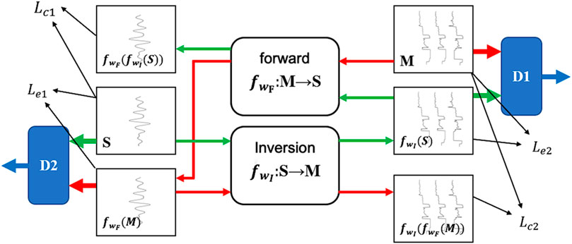
Figure 1. The CycleGAN inversion network architecture. The network comprises two generators and two discriminators, labeled as D₁ and D₂. The generators are tasked with forward modeling of seismic data and inversion of reservoir parameters, while the discriminators evaluate the authenticity of the generated outputs.

The discriminator loss function is defined as follows.

$Lossfunction=\mathit{log}\left(\mathrm{D}\left(x\right))+\mathit{log}(1-\mathrm{D}\left(\mathrm{G}\left(z\right)\right)\right)$

which represents the discriminator D(x) on the discrimination result from the real sample, and D (G(z)) represents the discriminator on the discrimination result from the sample generated by the generator. Following the workflow in Figure 1, we rewrite D(x) and 1-D (G(z)) in the above formulas into the following specific parameters to demonstrate a binary game process for finding the maximum and minimum, to ensure that the basic features of the prediction results for unlabeled seismic data are the same as those of the actual data. The discriminator loss, resembling a min-max two-player game, can be expressed as follows.

$\begin{array}{ll}\hfill \underset{W_I}{\min }\underset{W_{D1}}{\max }{L}_{D1}& =\mathit{log}{f}_{W_{D1}}\left(M\right)+\mathit{log}\left(1-f_{W_{D1}}\left(f_{W_I}\left(S\right)\right)\right)\hfill \\ \hfill & +\mathit{log}\left(1-f_{W_{D1}}\left(f_{W_I}\left(S^{*}\right)\right)\right)\hfill \end{array}$

$\underset{W_F}{\min }\underset{W_{D2}}{\max }{L}_{D2}=\mathit{log}{f}_{W_{D2}}\left(S\right)+\mathit{log}{f}_{W_{D2}}\left(S^{*}\right)+\mathit{log}\left(1-f_{W_{D2}}\left(f_{W_F}\left(M\right)\right)\right)$

The goal of the discriminator loss function is to maximize the discriminative result of the real sample (D(x)) while minimizing the discriminative result of the generated sample (D (G(z))). In this way, the discriminator can gradually improve its ability to discriminate real samples and thus better distinguish between real and generated samples. The discriminator loss L_D1 ensures that the basic characteristics of the predicted results for unlabeled seismic data are consistent with the actual data. This component plays a crucial role in maintaining the reliability and accuracy of CycleGAN’s predictions.

As indicated in Figure 1, CycleGAN is a game process, in which there is a competitive and cooperative relationship between the discriminator and the generator, and the discriminator loss function provides feedback signals to the generator, telling the generator the gap between the generated samples and the real samples. By minimizing the discriminator loss function, the generator can gradually generate samples that are closer to the real samples and improve the quality of the generated samples. The discriminator loss function drives this gaming process by maximizing the discriminative results of the real samples and minimizing the discriminative results of the generated samples, helping CycleGAN achieve dynamic equilibrium.

1.2 Generator network model

The CycleGAN structure is distinguished from other GANs by having an additional generator and discriminator, which enables it to be configured for semi-supervised learning. In this study, a one-dimensional AlexNet (Krizhevsky et al., 2012) is used as a discriminator capable of producing binary output for the binary output, and GRU as well as ResNet are added to the generator network structure. Residual networks, due to their internal residual blocks that employ skip connections, mitigate the gradient vanishing problem associated with increasing depth in deep neural networks (He et al., 2016). To solve the long-time dependency problem, Cho et al. proposed the GRU, an enhancement of RNNs that improves the filtering of past information. The correlation between seismic information across different strata makes GRU a suitable choice for solving inversion problems.

As shown in Figure 2, the generator network consists of three parts. Initially, seismic data is input in parallel to a module comprising three serially connected GRUs and three residual blocks with different dilation coefficients. The objective here is twofold: to leverage the GRU’s capability to capture long-term dependencies for extracting global features from seismic data, and to use the residual blocks for extracting local features at different scales from the seismic data, subsequently merging these local features using fully connected layers and convolutional blocks. The convolutional block in this study is composed of one-dimensional convolutional layers, batch normalization layers, and ReLU activation functions. Subsequently, the extracted local and global features are combined and input into a deconvolution block. The purpose of this block is to upsample the resized input data back to its original sampling rate. Finally, the data is input into a series of convolutional blocks to map the data from the feature domain to the target domain, i.e., from seismic data to elastic parameters.

Figure 2

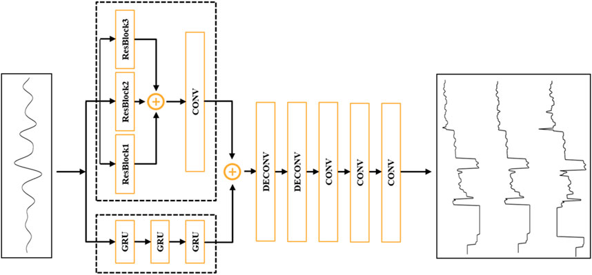
Figure 2. Generator network architecture incorporating GRU to model the relationship between seismic data and elastic impedance.

1.3 Establish geophysical constraint method

Pre-stack three-parameter inversion can be expressed as

$S=G\left(M\right)+n$

Here, S represents seismic data, M denotes elastic parameters, G is the mapping relationship between them, and n is noise. The essence of the neural network inversion method is to learn the mapping relationship between seismic data and elastic parameters from a given labeled dataset. As the Hybrid-Geophysics-Data (HGD) model shown in Figure 3, initial wave elastic parameter values are first obtained using deterministic inversion. These values are then mixed with labeled data to form the neural network’s training set, aiming to predict more accurate results.

Figure 3

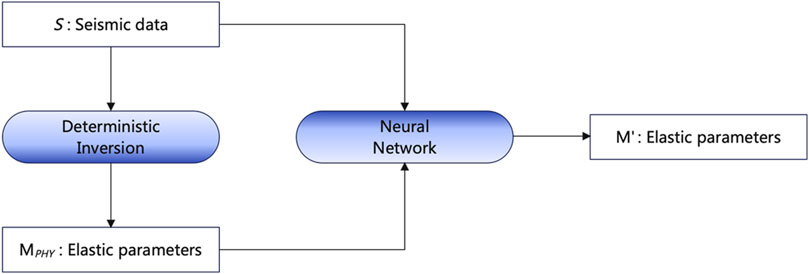
Figure 3. A schematic illustration of a basic Hybrid-Geophysics-Data (HGD) model. This model uses neural networks to establish the relationship between seismic data and elastic parameters.

In general regression problems, the loss function of a network is calculated using the difference between the predicted values and the sample’s label values.

$loss=L\left(net\left(x\right),y^{label}\right)=L\left(y^{pred},y^{label}\right)$

Here, $L$ represents the calculation formula of the loss function, $x$ is the network input, $net$ represents the network’s prediction process, $y^{pred}$ ​is the result obtained from processing $x$ through $net$, and $y^{label}$ is the sample’s label value. However, the training process of such networks is heavily influenced by the training set and lacks geophysical constraints. Therefore, this study incorporates the results of forward modeling of geophysical equations as constraints into the neural network’s loss function, ensuring that the predictions align more closely with geophysical principles. The workflow diagram of the loss function with geophysical constraints is shown in Figure 4.

Figure 4

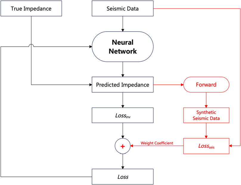
Figure 4. Flowchart of the SeisInv-CycleGAN loss function with geophysical constraints. SeisInv-CycleGAN uses the traditional forward modeling process to replace the generator used for forward modeling under the original CycleGAN structure. This can not only add geophysical constraints to the network, but can also significantly reduce network training time.

In a pre-stack inversion, the loss function uses Mean Squared Error (MSE), which can be expressed as

$loss=MSE\left(M_i^{pred},M^{true}\right)=\frac{1}{N}{\displaystyle {\sum }_{i=1}^N}{\left(M_i^{pred}-M_i^{true}\right)}^2$

Here, $N$ represents the number of samples, $M^{pred}$ is the elastic parameter value predicted by the network, $M^{true}$​ is the true elastic parameter value of the sample, and $MSE$ denotes the Mean Squared Error function. The synthetic seismic data calculated from the predicted $M^{pred}$​ using the forward modeling process is compared with the model seismic data using $MSE$. The residual between these two sets of data is used as a model-constrained loss term in the seismic inversion problem and is referred to as seismic loss. Thus, a complete loss function with geophysical constraints is obtained.

$\begin{array}{l}loss=los{s}_{inv}+\lambda los{s}_{seis}\\ =MSE\left(Z_i^{pred},Z_i^{true}\right)+\lambda *MSE\left(sei{s}_i^{pred},sei{s}_i^{true}\right)\end{array}$

Here, ${loss}_{inv}$ represents the $MSE$ loss function between the network-predicted elastic parameters and the true elastic parameters, and ${loss}_{seis}$ represents the $MSE$ loss function between the seismic records obtained from the forward modeling of the network-predicted elastic parameters and the true seismic records. $\lambda$ is a hyperparameter determining the weight ratio between the prediction loss and the seismic loss. The seismic loss addresses not only the labeled data but also can calculate the loss value for unlabeled data in other gathers, reducing the network’s dependency on labeled data and enhancing its generalization ability.

1.4 Workflow

The SeisInv-CycleGAN inversion framework, as shown in Figure 5, is built upon the base of CycleGAN, replacing the forward modeling network with a traditional forward modeling process. This substitution not only imposes geophysical constraints on the network but also significantly reduces the network training time. After replacing the generator, the generator responsible for forward modeling requires no training. As a result, the predicted loss of SeisInv-CycleGAN becomes

$L_e=\Vert M-f_{W_I}\left(S\right){\Vert }_2^2$

$L_{Seis}={\lambda }_{Seis}{L}_{c1}={\lambda }_{Seis}\left({‖S-f_{W_F}\left(f_{W_I}\left(S\right)\right)‖}_2^2+{‖S^{*}-f_{W_F}\left(f_{W_I}\left(S^{*}\right)\right)‖}_2^2\right)$

Figure 5

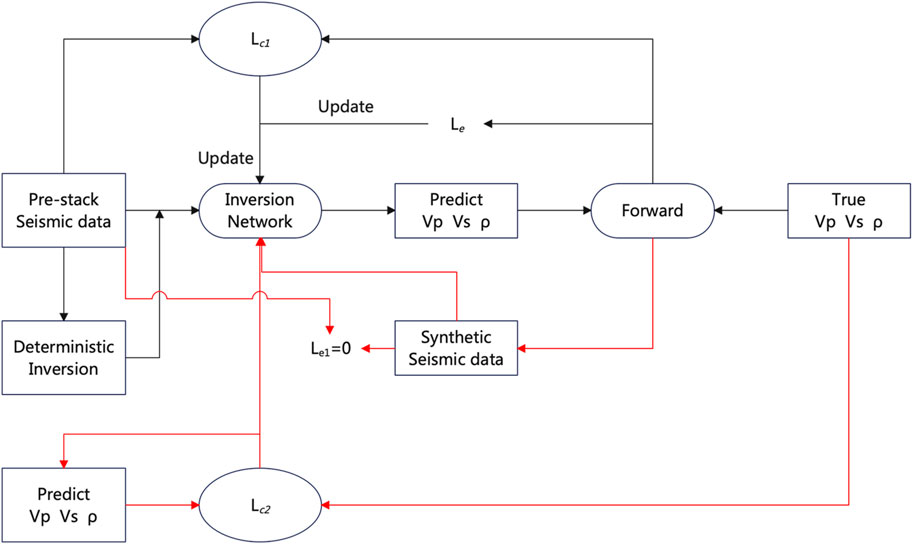
Figure 5. The workflow of SeisInv-CycleGAN. The SeisInv-CycleGAN is built upon the base of CycleGAN, replacing the forward modeling network with a traditional forward modeling process.

In the formula, ${\lambda }_{seis}$ is the weight parameter of $L_{c1}$. The ${\lambda }_{seis}$ added to $L_{seis}$ represents the loss function with geophysical constraints, and the size of ${\lambda }_{seis}$ determines the proportion of $L_{seis}$ in the entire loss function for subsequent evaluation.

When the network is trained, the generator network used for seismic inversion is extracted and used as the final network for predicting elastic parameters. As indicated in Figure 5, the input is the entire pre-stack seismic data, and the network outputs three elastic parameters: P-wave velocity, S-wave velocity, and density.

2 Model testing

This study selects the Marmousi-2 model as the experimental model to verify the advantages of the model-constrained optimized generative adversarial network seismic inversion method over other neural network-based methods.

2.1 Training dataset

The Marmousi-2 model is shown in Figure 6, with the parameters for the forward modeling part shown in Table 1. The Marmousi-2 model is a wave impedance model with a total of 2,721 channels, each channel has 470 sampling points, and the sampling rate is 1 m. Synthetic seismic data can be obtained through forward modeling of the convolution model. According to the convolution principle, seismic data can be calculated from wave impedance and seismic wavelets. The calculation formula is as follows.

$R_i=\frac{Z_{i+1}-Z_i}{Z_{i+1}+Z_i},Seis=W*R$

Figure 6

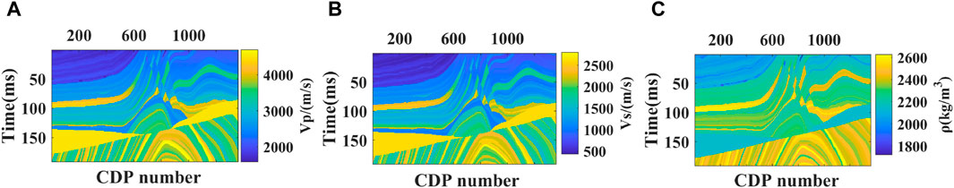
Figure 6. The Marmousi-2 model data. The Marmousi-2 model is a wave impedance model with a total of 2,721 channels. The figure shows the P-wave velocity (V_p), S-wave velocity (V_s), and density (ρ) of the Marmousi-2 model respectively. (A) P-wave velocity; (B) S-wave velocity; (C) density.

Table 1

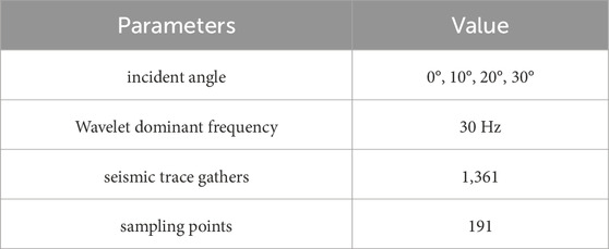
Table 1. Parameters used in forward modeling.

In the formula, Seis is seismic data, Z is wave impedance, W is seismic wavelet, and R is reflection coefficient. Among them, the main frequency of the wavelet is 30 Hz and the sampling rate is 1 m. In the neural network, seismic data is taken as input, and wave impedance is taken as output.

Synthetic seismic data are generated using the forward modeling process derived earlier. After normalizing the data, it is divided into training and testing sets.

To simulate real inversion problems, this model trial selects eight tracks (0.6% of the total samples) of labeled data as the training set. First, deterministic inversion is performed on the training set, and then the corresponding deterministic inversion results and labeled data are combined to form the network’s training set, enabling the network to train on diverse data to capture complex features.

Section 1.1 explains the loss function of Cycle-GAN, which can train on unlabeled seismic data to reduce reliance on labeled data. Therefore, 30 tracks of data are uniformly selected from non-labeled seismic data (as shown in Figure 7) to expand the training set, which initially contains only 15 labeled tracks.

Figure 7

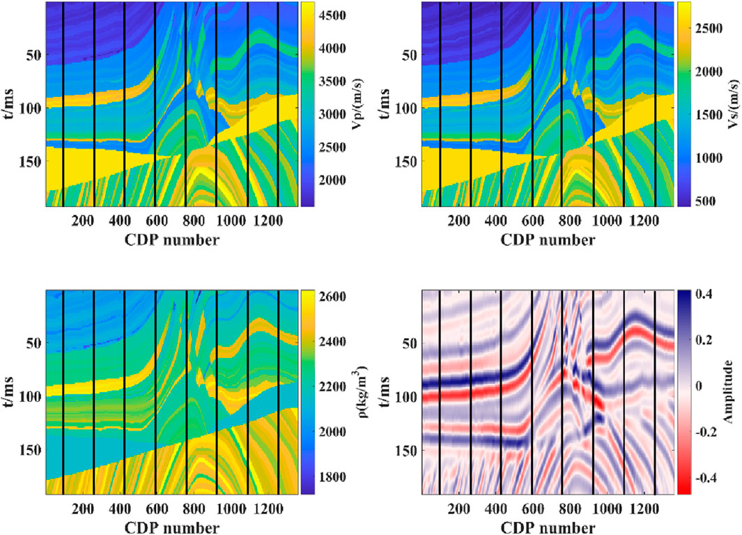
Figure 7. The location of the training set was selected from non-labeled training samples extracted from the seismic data of the Marmousi-2 model.

The goal of semi-supervised learning is to use non-labeled data to improve the model’s generalization performance. The training of non-labeled data is a self-training method conducted after training labeled data. The principle involves assigning approximate label values (pseudo-labels) to non-labeled data based on labeled data during the network training process. The training data is expanded by combining real labeled data and pseudo-labeled data to enhance the model’s generalization performance. The training process of the neural network is shown in Figure 8.

Figure 8

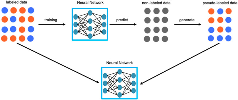
Figure 8. The training process of neural networks using non-labeled data. The goal of semi-supervised learning is to use non-label data to improve the generalization performance of the model. The training principle of non-label data is to give the approximate label value of the pseudo-label data based on the label data during the network training process. The training data is expanded by combining real labeled data and pseudo-labeled data to improve the model’s generalization performance.

2.2 Feasibility test

P-wave velocity, S-wave velocity, and density are three basic elastic parameters characterizing a reservoir, and pre-stack inversion is one of the most common methods to obtain these parameters. However, due to the band-limited nature of seismic data, noise in seismic records, and inaccuracies in the forward modeling, pre-stack inversion is generally an ill-posed problem, leading to unstable inversion results (Yang and Yin, 2008; Feng, 2019). Despite advances in AVO inversion and other technologies making the elastic parameters obtained from pre-stack inversion increasingly accurate, most scholars still find it challenging to achieve stable and high-precision density inversion results (Li et al., 2019). Therefore, we focus on the prediction of elastic parameters such as density using deep learning methods.

To validate the feasibility of the proposed method, a single-track comparison is made between the SeisInv-CycleGAN prediction results and the results from deterministic inversion, as shown in Figure 9. In the figure, the blue line represents the true values, the red line represents the network prediction results, and the black line represents the deterministic inversion results. It can be seen that both the deterministic inversion and SeisInv-CycleGAN predictions for P-wave and S-wave velocities closely match the true values, with SeisInv-CycleGAN having slightly higher accuracy. However, as mentioned earlier, the density curves calculated using deterministic inversion deviate significantly from the model data and are unstable. The SeisInv-CycleGAN prediction of density, similar to its prediction of P-wave and S-wave velocities, directly establishes a mapping relationship with seismic data. Therefore, the SeisInv-CycleGAN density prediction results, like those for P-wave and S-wave velocities, show a high degree of fit with the model data curves. In summary, using the proposed SeisInv-CycleGAN for pre-stack three-parameter synchronous inversion yields results superior to traditional deterministic inversion. Next, a comprehensive comparison will be conducted between the CycleGAN inversion method and the proposed method in terms of prediction accuracy and stability.

Figure 9

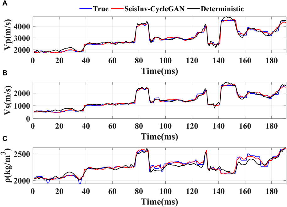
Figure 9. The comparison of single seismic trace between deterministic inversion results and SeisInv-CycleGAN prediction results. (A) P-wave velocity; (B) S-wave velocity; (C) Density.

2.3 Model test under noise-free conditions

To validate the performance of the proposed method, a comparative analysis of CycleGAN and SeisInv-CycleGAN is conducted in three aspects: prediction result profiles (Figure 10), absolute errors between prediction results and model data (Figure 11), and single-track comparison at CDP 200 and 1,100 (Figure 12). Additionally, average values of Pearson Correlation Coefficient (PCC), R-squared (R²), and Mean Squared Error (MSE) were calculated as quantitative indicators to evaluate network performance. Tables 2, 3 present the average PCC, R², and MSE values for the prediction results of CycleGAN and SeisInv-CycleGAN.

Figure 10

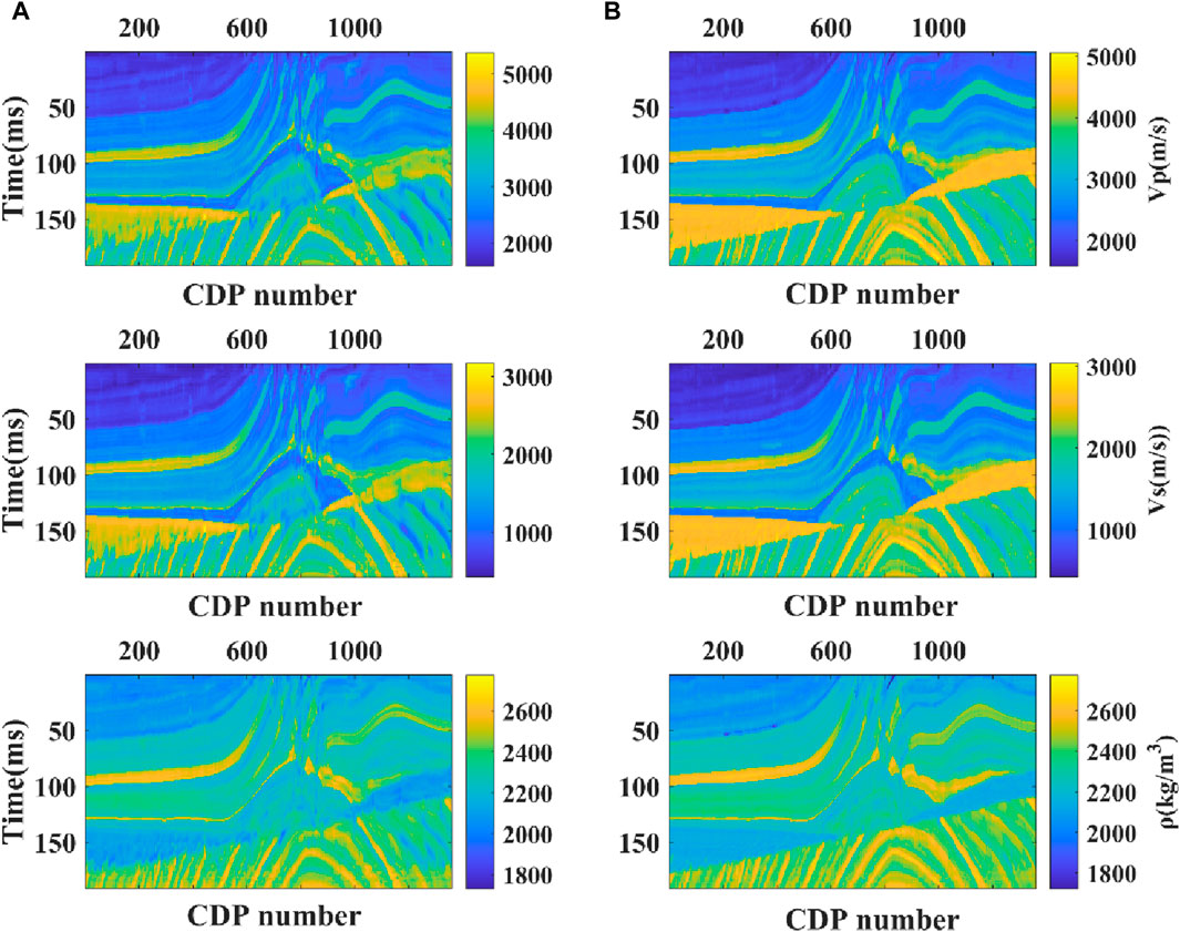
Figure 10. The prediction results of different networks under noise-free conditions with a comparative analysis of CycleGAN and SeisInv-CycleGAN. (A) CycleGAN; (B) SeisInv-CycleGAN.

Figure 11

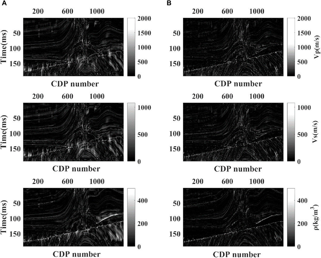
Figure 11. The absolute errors between different network prediction profiles and model data under noise-free conditions with a comparative analysis of CycleGAN and SeisInv-CycleGAN. (A) CycleGAN; (B) SeisInv-CycleGAN.

Figure 12

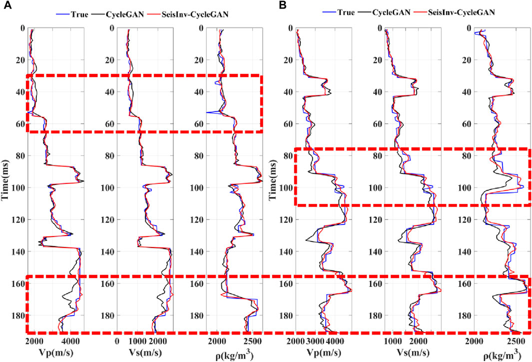
Figure 12. The comparison of single seismic traces of different network under noise-free conditions. (A) CDP=200; (B) CDP=1,100.

Table 2

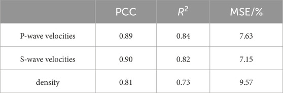
Table 2. The quantitative evaluation of the CycleGAN prediction results.

Table 3

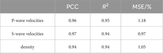
Table 3. The quantitative evaluation of the SeisInv-CycleGAN prediction results.

The analysis and comparison of the above-mentioned figures and tables show that SeisInv-CycleGAN outperforms CycleGAN in all metrics. Although CycleGAN, as a semi-supervised learning neural network, can learn features from unlabeled seismic data and predict results close to model data in the case of insufficient labeled data, it shows large deviations in predictions at complex geological structures and faults where velocity changes abruptly, with significant lateral jitters in overall predictions. This is attributed to the lack of geophysical constraints in CycleGAN, resulting in a lower correlation between predictions and model data, leading to the mentioned issues. SeisInv-CycleGAN, an improvement upon CycleGAN with an enhanced generator network and two geophysical constraints, shows notably better prediction accuracy, with minor deviations in predictions at complex structures and faults. The PCC and R² values for all three predicted parameters in SeisInv-CycleGAN exceed 0.94.

2.4 Model test under noise conditions

To test the noise resistance of SeisInv-CycleGAN, seismic data with Signal-to-Noise Ratios (SNRs) of 2, 5, and 10 were input into the trained network.

Table 4 presents the average PCC, R², and MSE values for the prediction results of the SeisInv-CycleGAN under noise conditions. Taking the PCC value as an example, it can be seen from Table 4 that the PCC value of SeisInv-CycleGAN is greatly improved compared to Cycle-GAN, and the accuracy of the prediction results is improved more obviously, which indicates that the inclusion of geophysical information greatly improves the prediction accuracy.

Table 4

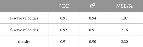
Table 4. The quantitative evaluation of the SeisInv-CycleGAN prediction results.

The network’s prediction results are shown in Figures 13, 14, with a single-track comparison at CDP=200 shown in Figure 15. From the prediction profile, it is evident that the profile at SNR=10 is broadly similar to the noise-free prediction profile, SNR=5 slightly impacts the accuracy of the predictions with the main structural forms remaining relatively clear, and SNR=2 results in a more blurred prediction profile with significant fluctuations at faults and unconformities. The single-track comparison shows that the green curve at SNR=10 is more stable and accurate in value prediction than the yellow curve at SNR=5 and the black curve at SNR=2, and is closer to the red curve representing noise-free seismic data predictions. This demonstrates the strong noise resistance of SeisInv-CycleGAN; at SNRs around 10 or higher, the network’s predictions are almost unaffected. At SNRs around 5, the accuracy of the predictions is slightly reduced but within an acceptable range. At SNRs of two or lower, the strong noise signal leads to slightly poorer network predictions, and noise suppression processing may be required before inversion.

Figure 13

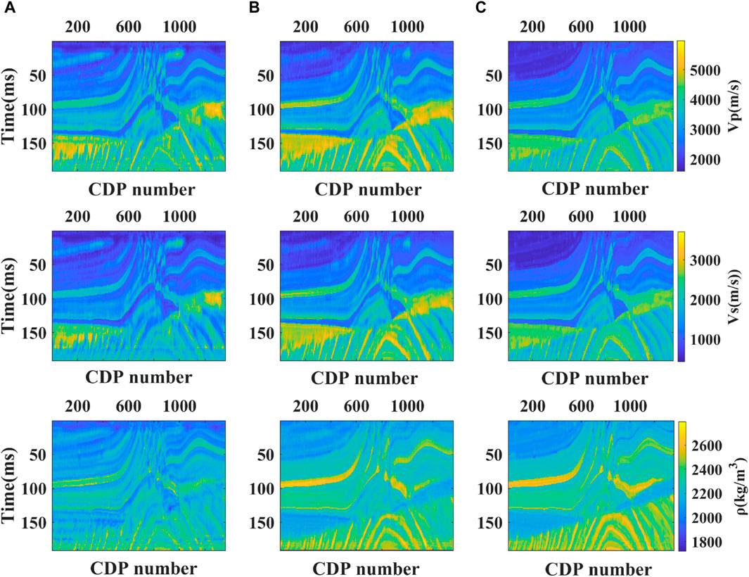
Figure 13. The predicted profiles of seismic data with different signal-to-noise ratios. (A) SNR=2; (B) SNR=5; (C) SNR=10.

Figure 14

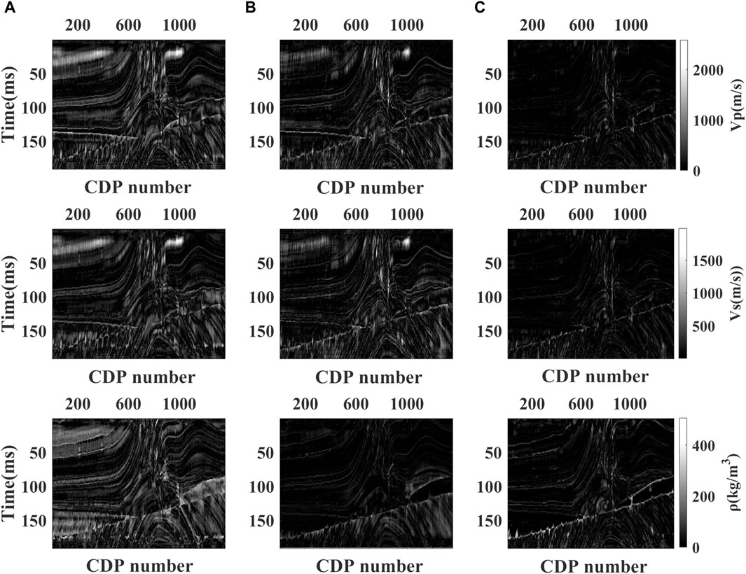
Figure 14. The absolute errors between predicted profiles and model data using seismic data with different signal-to-noise ratios (SeisInv-CycleGAN). (A) SNR=2; (B) SNR=5; (C) SNR=10.

Figure 15

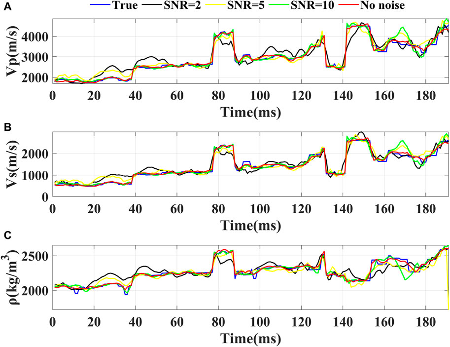
Figure 15. The predicted results of seismic data with different signal-to-noise ratios. (A) P-wave velocity; (B) S-wave velocity; (C) Density.

3 Conclusion

In this study, SeisInv-CycleGAN, a physically-guided cycle-consistent generative adversarial network architecture based on physical guidance, is proposed to realize high-precision pre-stacked multi-parameter simultaneous inversion of a small amount of labeled data by improving the structure of the generator network in CycleGAN, replacing its orthogonal network with a geophysical orthogonal one, and adding two kinds of geophysical constraints. From the pre-stack multi-parameter synchronous inversion model trials using the Marmousi model, it is evident that using a generator network constructed with ResNet and GRU significantly enhances the capability to extract features from labeled data. Employing a hybrid geophysical data model and a loss function constrained by geophysical principles effectively limits the neural network’s training process, substantially improving its predictions’ accuracy. Furthermore, the applicability of this framework is not confined to the pre-stack three-parameter inversion of the Marmousi model but can be extended to new research areas such as anisotropic parameter inversion.

Data availability statement

The original contributions presented in the study are included in the article/Supplementary material, further inquiries can be directed to the corresponding author.

Author contributions

GZ: Conceptualization, Data curation, Funding acquisition, Investigation, Project administration, Writing–original draft, Writing–review and editing, Formal Analysis, Methodology, Software. SS: Investigation, Software, Writing–original draft, Writing–review and editing, Data curation, Methodology. HZ: Conceptualization, Data curation, Writing–original draft, Writing–review and editing, Investigation, Methodology. DC: Validation, Visualization, Writing–review and editing, Resources.

Funding

The author(s) declare that financial support was received for the research, authorship, and/or publication of this article. We would like to acknowledge the sponsorship of the National Natural Science Foundation of China (U23B6010, 42074136).

Conflict of interest

Author HZ was employed by Tianjin Survey and Design Institute for Water Transport Engineering Co Ltd. Author DC was employed by PetroChina.

The remaining authors declare that the research was conducted in the absence of any commercial or financial relationships that could be construed as a potential conflict of interest.

Publisher’s note

All claims expressed in this article are solely those of the authors and do not necessarily represent those of their affiliated organizations, or those of the publisher, the editors and the reviewers. Any product that may be evaluated in this article, or claim that may be made by its manufacturer, is not guaranteed or endorsed by the publisher.

References

Alfarraj, M., and AlRegib, G. (2019). Semisupervised sequence modeling for elastic impedance inversion. Interpretation 7 (3), 237–249. doi:10.1190/int-2018-0250.1

CrossRef Full Text | Google Scholar

An, P., Cao, D., Zhao, B., Yang, X., and Zhang, M. (2019). Research on reservoir physical parameter prediction method based on LSTM recurrent neural network. Prog. Geophys. 34 (05), 1849–1858. doi:10.6038/pg2019CC0366

CrossRef Full Text | Google Scholar

Cai, A., Di, H., Maniar, H., and Abubakar, A. (2020). Wasserstein cycle-consistent generative adversarial network for improved seismic impedance inversion: example on 3D SEAM model. Houston, Texas, United States: SEG Technical Program Expanded Abstracts, 1274–1278.

Google Scholar

Das, V., Pollack, A., Wollner, U., and Mukerji, T. (2019). Convolutional neural network for seismic impedance inversion. Geophysics 84 (6), R869–R880. doi:10.1190/geo2018-0838.1

CrossRef Full Text | Google Scholar

Feng, Q. (2019). Research on pre-stack density inversion methods. Energy Environ. 41 (06), 57–61. doi:10.19389/j.cnki.1003-0506.2019.06.012

CrossRef Full Text | Google Scholar

He, K., Zhang, X., Ren, S., and Sun, J. (2016). “Identity mappings in deep residual networks,” in European conference on computer vision, Amsterdam, The Netherlands, October, 2016, 630–645.

CrossRef Full Text | Google Scholar

Hinton, G., and Salakhutdinov, R. (2006). Reducing the dimensionality of data with neural networks. Science 313, 504–507. doi:10.1126/science.1127647

PubMed Abstract | CrossRef Full Text | Google Scholar

Krizhevsky, A., Sutskever, I., and Hinton, G. (2012). ImageNet classification with deep convolutional neural networks. Adv. Neural Inf. Process. Syst. 25 (2). doi:10.1145/3065386

CrossRef Full Text | Google Scholar

Li, J., Yin, C., Liu, X., Chen, C., and Wang, M. (2019). Pre-stack density stable inversion method for shale reservoirs. Chin. J. Geophys. 62 (05), 1861–1871. doi:10.6038/cjg2019M0356

CrossRef Full Text | Google Scholar

Li, L., Wen, X., Liu, S., Ran, X., Huang, W., and Li, B. (2019). Pre-stack seismic inversion based on approximate equations of two reflection coefficients of longitudinal and transverse wave moduli. Prog. Geophys. 34 (02), 581–587. doi:10.6038/pg2019CC0035

CrossRef Full Text | Google Scholar

Liu, J., Wen, X., Zhang, Y., and Wu, H. (2022). Pre-stack seismic inversion of igneous rock reservoir physical parameters. Prog. Geophys. 37 (5), 1985–1992. doi:10.6038/pg2022FF0452

CrossRef Full Text | Google Scholar

Pan, X., and Zhang, G. (2019). Fracture detection and fluid identification based on anisotropic Gassmann equation and linear-slip model. Geophysics 84 (1), R85–R98. doi:10.1190/geo2018-0255.1

CrossRef Full Text | Google Scholar

Pan, X., Zhang, G., and Cui, Y. (2020). Matrix-fluid-fracture decoupled-based elastic impedance variation with angle and azimuth inversion for fluid modulus and fracture weaknesses. J. Petroleum Sci. Eng. 189, 106974. doi:10.1016/j.petrol.2020.106974

CrossRef Full Text | Google Scholar

Pan, X., Zhang, G., and Yin, X. (2017). Azimuthally anisotropic elastic impedance inversion for fluid indicator driven by rock physics. Geophysics 82 (6), C211–C227. doi:10.1190/geo2017-0191.1

CrossRef Full Text | Google Scholar

Pan, X., and Zhao, Z. (2024). A decoupled fracture- and stress-induced PP-wave reflection coefficient approximation for azimuthal seismic inversion in stressed horizontal transversely isotropic media. Surv. Geophys. An Int. Rev. J. Geophys. Planet. Sci. 45, 151–182. doi:10.1007/s10712-023-09791-y

CrossRef Full Text | Google Scholar

Pan, X., Zhao, Z., and Zhang, D. (2023). Characteristics of azimuthal seismic reflection response in horizontal transversely isotropic media under horizontal in situ stress. Surv. Geophys. An Int. Rev. J. Geophys. Planet. Sci. 44, 387–423. doi:10.1007/s10712-022-09739-8

CrossRef Full Text | Google Scholar

Phan, S., and Sen, M. K. (2018). Hopfield networks for high-resolution prestack seismic inversion. Houston, Texas, United States: SEG Technical Program Expanded Abstracts. Society of Exploration Geophysicists, 526–530.

Google Scholar

Röth, G., and Tarantola, A. (1994). Neural networks and inversion of seismic data. J. Geophys. Res. Solid Earth 99 (B4), 6753–6768. doi:10.1029/93jb01563

CrossRef Full Text | Google Scholar

Song, L., Yin, X., Zong, Z., Li, B., Qu, X., and Xi, X. (2021). Seismic wave impedance inversion method based on deep learning with prior constraints. Geophys. Prospect. Petroleum 56 (04), 716–727. doi:10.13810/j.cnki.issn.1000-7210.2021.04.005

CrossRef Full Text | Google Scholar

Wang, J., Wen, X., He, Y., Lan, Y., and Zhang, C. (2022a). Log curve prediction method based on CNN-GRU neural network. Geophys. Prospect. Petroleum 61 (02), 276–285. doi:10.3969/j.issn.1000-1441.2022.02.009

CrossRef Full Text | Google Scholar

Wang, Y., Ge, Q., Lu, W., and Yan, X. (2019). Seismic impedance inversion based on cycle-consistent generative adversarial network. Houston, Texas, United States: SEG Technical Program Expanded Abstracts 2019. Society of Exploration Geophysicists, 2498–2502.

Google Scholar

Wang, Y., Wang, Q., Lu, W., Ge, Q., and Yan, X. F. (2022b). Seismic impedance inversion based on cycle-consistent generative adversarial network. Petroleum Sci. 19 (1), 147–161. doi:10.1016/j.petsci.2021.09.038

CrossRef Full Text | Google Scholar

Wang, Z., Xu, H., Yang, M., and Zhao, Y. (2022c). Seismic wave impedance inversion method using time domain convolutional neural network. Geophys. Prospect. Petroleum 57 (02), 279–286. doi:10.13810/j.cnki.issn.1000-7210.2022.02.004

CrossRef Full Text | Google Scholar

Yang, L., Wu, Y., Wang, J., and Liu, Y. (2018). A review of recurrent neural networks. Comput. Appl. 38 (S2), 1–6.

Google Scholar

Yang, P., and Yin, X. (2008). A review of seismic wavelet extraction methods. Geophys. Prospect. Petroleum (01), 123–128. doi:10.3321/j.issn:1000-7210.2008.01.021

CrossRef Full Text | Google Scholar

Yin, X., Wu, G., and Zhang, H. (1994). Application of neural networks in lateral prediction of reservoirs. J. China Univ. Petroleum Ed. Nat. Sci. 018 (005), 20–26.

Google Scholar

Yu, S., and Ma, J. (2021). Deep learning for geophysics: current and future trends. Rev. Geophys. 59 (3). doi:10.1029/2021rg000742

CrossRef Full Text | Google Scholar

Zhang, H., Zhang, G., Gao, J., Li, S., Zhang, J., and Zhu, Z. (2022a). Seismic impedance inversion based on geophysical-guided cycle-consistent generative adversarial networks. J. Petroleum Sci. Eng. 218, 111003–111011. doi:10.1016/j.petrol.2022.111003

CrossRef Full Text | Google Scholar

Zhang, S., Si, H., Wu, X., and Yan, S. (2022b). A comparison of deep learning methods for seismic impedance inversion. Petroleum Sci. 19 (3), 1019–1030. doi:10.1016/j.petsci.2022.01.013

CrossRef Full Text | Google Scholar

Zhao, C., and Gui, Z. (2005). Reservoir parameter prediction method and application based on neural networks. J. Oil Nat. Gas J. Jianghan Petroleum Inst. 27 (3), 467–468.

Google Scholar

Zhou, Y., Zhang, G., Zhang, S., Liu, J., and Han, L. (2022). Prediction method of tight reservoir fracture openness based on hierarchical expert committee machine model. Geophys. Prospect. Petroleum 57 (02), 287–296. doi:10.13810/j.cnki.issn.1000-7210.2022.02.005

CrossRef Full Text | Google Scholar