External factors driving surface temperature changes above geothermal systems: answers from deep learning

Introduction: The surface expression of enhanced geothermal heat fluxes above an active hydrothermal system causes a surface thermal anomaly (ΔT). The thermal anomaly is expressed by the difference between the temperature within the heated zone (T_h) and the temperature of non-heated surfaces (T₀). Given that the resulting thermal anomaly at the surface is of extremely low magnitude (1°C–5°C at Vulcano, Italy), it is extremely sensitive to overprinting by external factors, namely, meteorological influences on surface temperature variation, such as solar heating, wind and rain.

Methods: To test the sensitivity of the surface to external drivers, we installed two surface temperature measurement stations within the Vulcano’s Fossa crater, one inside the thermal anomaly and one outside (separation = 50 m), with a weather station co-located with the T₀ station. Time series of T_h and T₀ were collected for 2020, when the Vulcano Fossa hydrothermal system was at a low and stable level of activity so that external drivers would have been the main influences on T_h and T₀, and hence also ΔT. To test for divergence from normality in terms of diurnal and seasonal variations in T_h and T₀, and the role of external factors in causing abnormality, we used the deep learning engine DITAN: a domain-agnostic framework to detect and interpret anomalies in time-series data.

Results: During the year, DITAN found 16 cases of two types of meteorological events: intense low-pressure systems and high-intensity rainstorms (cloudbursts). Passage of 13 abnormal low-pressure systems were detected (10 between February and May, and three in December), with three abnormal rainstorm events (all in December); all three being coincident with the abnormal low pressure events. We find just two abnormalities in the time series for of T_h and T₀, both of which coincide with passage of abnormal low-pressure systems, and neither of which coincide with abnormal rain events. We conclude that diurnal and annual heating and cooling cycles, subject to normal meteorological inputs and at a surface above a geothermal-heated source, are immune to anomalous behaviour to the external (meteorological) variations.

1 Introduction

A “geothermal system” is defined by Hochstein and Browne (2000) as a cascading system through which “natural heat transfer within a confined volume of the Earth’s crust where heat is transported from a heat source to a heat sink.” Geothermal systems are located in areas where heat flow is enhanced and where the structural setting allows for fluid circulation, such as at convergent plate margins, spreading centers, rift systems and mantle hot spots (Stimac et al., 2015). Geothermal systems not associated with a magmatic source have been termed by Nicholson and Nicholson (1993) “non-volcanic geothermal systems” and can be found in active tectonic areas where heat can be produced by deep water circulation in a faulting context. However, if the heat source is provided by magma, we have a “volcanic geothermal system” (Nicholson and Nicholson, 1993). In a volcanic geothermal system, heat and mass are transferred to the surface from a magma reservoir (Hochstein, 2005), where ascending magmatic fluids mix with descending fluids from the near-surface groundwater system to create a “volcanic-hydrothermal system”, hereafter termed “hydrothermal system”. A hydrothermal system is thus a system with four key components (Figure 1):

• a heat source (the magmatic source),

• an area of recharge (i.e., a “hydrothermal reservoir” of highly permeable rocks),

• an area of discharge (i.e., the “geothermal field” at the surface), and

• circulation of hydrothermal fluids contributing to mass and energy flows.

Figure 1

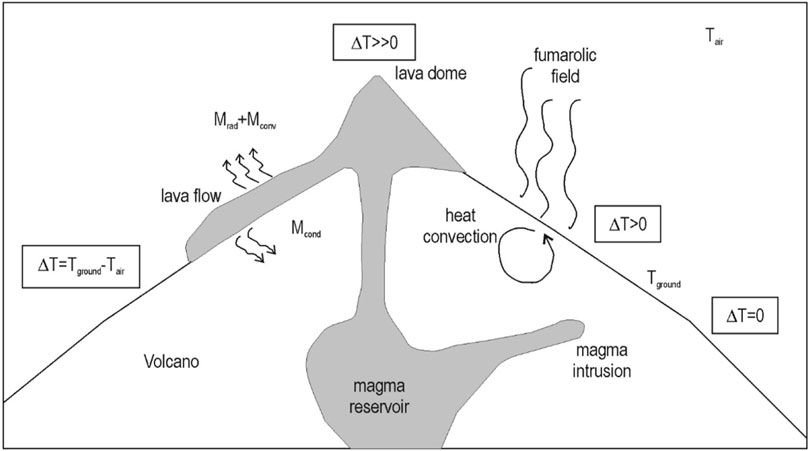
Figure 1. Figure 1 from chapter 0 of Harris (2013). Sketch of the main sources of thermal emission at a volcanic hydrothermal system, modified Figure 1 in Bonneville and Gouze (1992) and reproduced by permission of American Geophysical Union. In normal conditions ground (T_ground) and air temperature (T_air) are approximately equal, so that ΔT = T_ground − T_air ≈ 0. Over a subsurface heat supply, such as a magmatic intrusion above which natural convection in a porous, or fractured, medium carries heat to the surface, ΔT becomes positive. Over a high temperature surface heat source, such as an active lava, ΔT becomes strongly positive. The schematic also shows the main sources of heat loss from an active lava body. These being radiation (M_rad), convection (M_conv) and conduction (M_cond).

Diffuse heat fluxes from the hydrothermal system result in widespread and pervasive ground surface heating to cause a low amplitude (typically 1°C–10°C) thermal anomaly at the surface (e.g., Hochstein and Browne, 2000; Chiodini et al., 2005; Lagios et al., 2007; Aubert et al., 2008; Harris et al., 2009; Diliberto, 2011). The difference between the temperature of heated (T_h) and unheated ground (T₀) is here termed the thermal anomaly (Figure 1, ΔT = T_h − −T₀). Geothermally-heated surfaces are relatively cool compared to other active volcanic surfaces such as pyroclastic and lava flows, so that the associated thermal anomalies are just a few degrees centigrade above the ambient background (Figure 1). The low amplitude of thermal anomalies associated with hydrothermal systems make them difficult to detect and handle (Harris and Stevenson, 1997), and are likely to be extremely sensitive to external factors, especially meteorological factors such as rain, wind, humidity and atmospheric pressure. While low amplitude geothermal thermal anomalies are liable to dampening due to the cooling effect of rain and wind, radiative heat fluxes will be controlled by variations in water vapor pressure (e.g., Sekioka and Yuhara, 1974; Bahrami et al., 2019; Ishibashi et al., 2023), which is in turn controlled by humidity and atmospheric pressure. At such a low temperature system, forced or free convection will also be the dominant heat loss (Keszthelyi et al., 2003), where the convective heat transfer coefficient will depend on wind and air temperature (Harris, 2013).

We thus define the magmatic and hydrothermal reservoir components of the volcanic-hydrothermal system as internal sources that drive changes in surface temperature (T_h), and the atmospheric system as an external driver (Figure 3). To date, most studies have focused on the role of the magmatic source and the permeability of the hydrothermal reservoir in driving changes in temperature recorded at the surface (e.g., Dobson et al., 2003; Chiodini et al., 2005; Aubert et al., 2008; Harris et al., 2012). However, we are aware of no study that has focused purely on the potential role of external drivers on variation in T_h, T₀ and, hence, ΔT (Figure 1). Thus, to provide data capable of defining the role of external (meteorological) drivers on surface temperature variation above a hydrothermal system, we installed two surface-temperature measurement stations (to measure T_h and T₀), plus a weather station co-located with the T₀ station, inside Vulcano’s (Aeolian Islands, Italy) Fossa crater (Figure 2). In this regard Vulcano, being the host of a thermal anomaly associated with an active hydrothermal system and a well-monitored site (Chiodini et al., 2005; Harris et al., 2009), is an ideal laboratory to test hypotheses regarding the internal and external effects on the amplidude of DT.

Figure 2

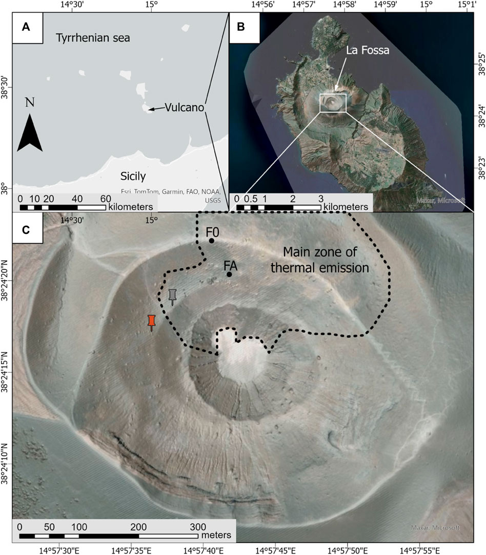
Figure 2. (A) Location of Vulcano in the Aeolian Island arc, and (B) of the Fossa on Vulcano, with (C) location of our measurement stations in respect to the heated zone in the Fossa crater. F0 and FA are the two main fumaroles, gray pin is the temperature station in the heated zone, and red pin is the co-located weather station and temperature station in the non-heated zone.

We installed the sensors in 2020, when levels of heat flux were particularly low so that the internal element of the system could be considered minimal and stable, and in a background or baseline state (Mannini et al., 2019; Pailot-Bonnétat et al., 2023). In such a state, temperature variations at the surface should be particularly sensitive to external drivers. However, given the sensitivity of temperature variation to both external and internal drivers (Figure 3), inter-relations between T_h, T₀ and external parameters will be complex, and any correlation will be extremely subtle. Such a multi-variate time series, in which there are unknown interactions between variables, is ideally suited to a machine learning (e.g., Malfante et al., 2018; Carniel and Guzmán, 2020; Watson et al., 2020). In particular, application of a deep learning-based approach to time series data can greatly aid in advancing volcano monitoring, and processing of volcanic geophysical and geochemical signals, especially when searching for patterns and interrelations in multi-sensor time series (e.g., Manley et al., 2022; Corradino et al., 2023; Ferreira et al., 2023).

Figure 3

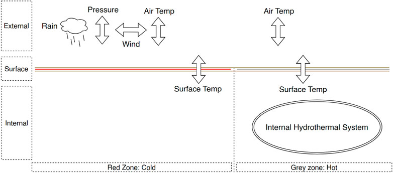
Figure 3. A descriptive illustration of the thermal system at Vulcano and its parameters.

We thus focus on isolating and defining those external drivers that change the surface thermal state of ground above a hydrothermal system in an abnormal fashion, our research question being:

Can, and if so how, do meteorological factors impinge on surface thermal anomalies above geothermal systems?

To do this we apply the deep learning framework DITAN (Giannoulis et al., 2023) to time series data for surface temperature and meteorological conditions collected in-situ at the active hydrothermal system at Vulcano (Pailot-Bonnétat and Harris, 2024), in an experiment designed to answer the stated research question. We begin by describing the characteristics of the study site (Vulcano) and the instrumentation installed there, before reviewing DITAN, its performance and output. In effect, this is the third in a three part series of papers where we have first set-up, tested and cross-validated DITAN in Giannoulis et al. (2023), and then (second) set up the experiment and data collection design in Pailot-Bonnétat and Harris (2024).

2 Background and data

At Vulcano, the magmatic source has been placed at a depth of 2–3 km by Ferrucci et al. (1991), and the magmatic contribution to the fumarolic gases has been established from chemical composition (Nuccio et al., 1999). The gas signature at Vulcano thus results from mixing of magmatic and hydrothermal fluids (marine and meteoritic), with the hydrothermal system being described as a biphase (water–vapor) boiling saline solution with a central vapor-monophase zone (e.g., Carapezza et al., 1981; Chiodini et al., 1995; Nuccio et al., 1999). Heat ascends from the mixing zone, which has its depth ≈1 km below the Fossa Crater (Nuccio et al., 1999; Alparone et al., 2010) to form a “heat pipe” (White et al., 1971) at the top of which there is a bottom-heated surface zone (Figure 2C). Heat loss from the heated surface is partitioned between the conductive flux through diffuse soil emissions and advection at fumarole vents (Sekioka and Yuhara, 1974; Chiodini et al., 2005; Harris, 2013). Heat flux from the zone of soil emission accounts for 93% ± 2% of the total energy budget, is defined by a thermal anomaly (ΔT) of 1°C–5°C (Harris et al., 2009; Mannini et al., 2019), and is associated with vertical gradients in the temperature profile within 1 m of the surface 50–135 K/m (Aubert et al., 2008).

At Vulcano, heat fluxes during the period 2010 to 2020 were particularly low and stable at around 4–12 MW, as was ΔT (Mannini et al., 2019). The period 2010–2020 has thus been defined as a baseline or background level for heat flux, against which change in the thermal state of the hydrothermal system can be assessed (Pailot-Bonnétat et al., 2023). We thus chose the year 2020 on which to target our study so as to determine external drivers on ΔT with the system in its background state. At Vulcano, the value of understanding system behaviour during such baseline studies was highlighted by the unrest that followed our period of interest. This new phase of unrest began in September 2021 and continued into 2022, and during which heat fluxes increased to peaks of around 120 MW (Pailot-Bonnétat et al., 2023).

Within the Fossa, in the vertical sense, there are thus two elements to the system that need to be constrained: 1) the immediate subsurface where enhanced geothermal heat flux (internal driver) causes elevated surface temperatures and 2) the atmosphere where meteorological parameters (external drivers) modulate surface temperature (Figure 3). Horizontally, there are also two zones: one of which is heated from below, and one of which is not (Figure 2C). Thus, in our experiment set-up, the surface thermal state of the heated and non-heated zones are tracked by two sensors that monitor surface and air temperature, with external meteorological conditions being measured by a third sensor array (Figure 3).

We installed the sensor network in the Fossa crater in January 2020. The network consists of two temperature stations separated by 50 m, with one inside the heated zone and one in the non-heated zone, plus a weather station co-located with the latter station (Figure 2C). The experimental set-up, sensors and data sets used here are fully described in Pailot-Bonnétat and Harris (2024), and are summarized here in Table 1. The two temperature stations consisted of two thermocouples (Onset HOBO TMC1-HD, signal to noise ratio = 0.1°C) measuring surface temperature (T_s) and air temperature (T_a) at a height of 15 cm above the surface. The thermocouples were linked to an Onset HOBO U12-008 data logger (storage capacity = 43,000 measurements) with a sampling rate of one record every five-to-ten minutes. The weather station was an Onset HOBO H21-USB which measured atmospheric pressure (S-BPB-CM50), air temperature and relative humidity (S-THC-M002), wind speed (S-WSB-M003), and rainfall using a tipping bucket rain gauge (S-RGF-M002). These meteorological sensors were installed at ground level, and the sampling rate was one record per minute. The chosen period of analysis is 31 January 2020, 12:00:00, to 31 December 2020, 23:00:00, with data gaps existing due to the logger capacity being reached before download, which was a problem due to mobility restrictions during the COVID-19 pandemic period (Table 2).

Table 1

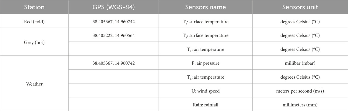
Table 1. The sensor network of Vulcano in year 2020.

Table 2

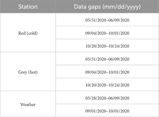
Table 2. Data gaps in the 2020 time series.

3 Methodology

Our sensor network provides a multivariate time series, in which each record is characterized by seven sensors, two sensors from the surface system and five sensors from the atmospheric (external) system (Figure 3). To learn the normal thermal behavior of the surface, and subsequently define externally-driven anomalies, we developed in Giannoulis et al. (2023) DITAN, a domain-agnostic deep learning based framework that is effective in detecting and interpreting temporal-based anomalies. A temporal-based anomaly, or simply anomaly, occurs when one or more sensor values (e.g., pressure and/or wind speed) deviate from their expected “normal” behavior. When this occurs on the full feature set, the anomaly is called full-space anomaly, otherwise sub-space anomaly if it applies to a sub feature set. When an anomaly persists for more than one record (e.g., two time steps) it is called sub-sequence anomaly. The severity score of an anomaly refers to the intensity of its contamination. Local anomalies typically receive lower scores due to their limited impact on the time series as a whole, being primarily confined to a specific region of the time-series. Global anomalies, conversely, tend to receive higher scores, indicating their widespread impact on the time series and significance across multiple data regions.

DITAN encompasses the integral temporal properties of a time series, built upon three assumptions: 1) the time series is predictable, 2) normality is identical to regularity, and 3) irregular records are temporally less predictable than regular records.

The model has been tuned using Bayesian optimization, to systematically search and exploit the range of values for various hyperparameters, aiming to determine the optimal configuration. Throughout this process, a forward chaining cross-validation was used to ensure that there is no leakage of information between the training and validation sets during the hyperparameter optimization phase.

In Giannoulis et al. (2023), the model has been deeply validated on six multivariate timeseries of varying anomalous types, using several performance metrics including confusion matrices, precision, recall and F_0.5 score. It has also been favorably compared to state of the art methods on anomaly detection.

DITAN is composed of four modules: 1) pre-processing, 2) domain-agnostic modeling, 3) application of a dynamic threshold with built-in pruning, and 4) numerical interpretation. We briefly describe here these four modules and refer the reader to Giannoulis et al. (2023) for further details.

3.1 Pre-processing

DITAN applies a series of steps to prepare a predictable multivariate time series in a favorable format for deep learning analysis. These steps include an optional decomposition of the sensor values into residuals or trends to focus on short-term or long-term regularities, respectively. Additionally, a mandatory min-max scaling is applied across sensors to maintain a common value range within [−3, 3]. A prediction-based protocol is used to forecast a horizon given a context. In this protocol, a horizon includes the estimation of the records within the context and the prediction of one or more subsequent records. Context-horizon mapping can then be seen as an “IF-THEN” rule, where the “IF” part needs to be estimated along with the prediction of the “THEN” part.

3.2 Domain-agnostic modeling

DITAN learns regularity across the context-horizon mappings using an LSTM encoder-decoder with attention mechanisms (Figure 4). LSTMs (Long Short-Term Memory) (Hochreiter and Schmidhuber, 1997) are a type of recurrent neural network (RNN) specially designed to model long-term dependencies in data sequences. Unlike traditional RNNs, LSTMs incorporate gating mechanisms, including forgetting, input and output gates, which enable them to regulate the flow of information through the network’s cells. These mechanisms enable LSTMs to capture and store important information over long periods of time, while mitigating the problems of gradient disappearance or explosion commonly encountered in conventional RNNs. Attention mechanisms (Luong et al., 2015) as for them enable the model to selectively focus on different parts of input data when making predictions. They allow DITAN to weigh the importance of different features or elements within the input, enhancing their ability to capture relevant information for the task at hand. This mechanism typically involves learning attention weights that dynamically allocate resources to different parts of the input.

Figure 4

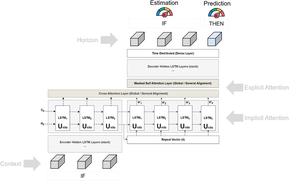
Figure 4. A graphical illustration of the DITAN architecture. The model is composed of LSTM layers along with a composite decoder and soft attention mechanisms to capture short-term and long-term normal (regular) patterns. The number of LSTM cells in the encoder (left) is equal to the context size, while the decoder (right) has a context sized number of LSTM cells to reconstruct, as well as a horizon sized number of LSTM cells to construct. Such a composite decoder forces the network to stay attentive to all time steps in the encoder, instead of only the last few steps. A full description of this model is proposed in Giannoulis et al. (2023).

In DITAN, the context is encoded in such a way that the decoder is responsible for both reconstructing the context and constructing the subsequent records. Each record is represented by an LSTM cell, which helps to memorize short-term relations. Additionally, each LSTM cell in the decoder explicitly attends to the encoder’s LSTM cells using a cross-attention layer. Moreover, a masked self-attention layer is employed to assess temporal weights based on the relative positions of the LSTM cells in the decoder. The structure of this architecture is optimized using the Bayes optimizer, which explores and exploits the value range of hyper-parameters with respect to the application features to select an optimal hyper-parameter configuration.

In the training phase, both estimation and prediction errors are utilized. An error eⁱ is computed as the difference between the forecasted (estimated or predicted) value xⁱ, and the observed value xⁱ for each sensor d in D. DITAN employs a configurable error function, which can be defined as either the squared $e_d^i=\Vert x_d^i-x_d^{i^{\prime }}{\Vert }_2$ or absolute $e_d^i=|x_d^i-x_d^{i^{\prime }}|$ error for all d ∈ D. The squared, as opposed to absolute, errors are non-linear weighted with respect to the error magnitude, and thus higher errors are magnified. The higher the error on a sensor value, the more abnormal the value is considered. A threshold is required to determine the turning point from normal to abnormal.

Recall that normality is equated to regularity, and irregular records are considered temporally less predictable than regular one. Consequently, during the training phase, the objective function of the model disregards context-horizon patterns that are contaminated by outliers and deemed irregular. These patterns, which constitute a small portion of the total number of patterns, are assigned a low weight and are effectively ignored.

3.3 Dynamic thresholding with built-in pruning

In the testing phase, only prediction errors are used. To determine the level of prediction error that records change from regular (normal) to irregular (abnormal), we use a thresholding methodology (Figure 5). Prediction errors are first smoothed to introduce locality. Next, all critical peaks are computed, which are peak values above the minimum peak height value. To find the minimum peak height value, we downhill the errors in the frequency space until we reach a bin in which variability is introduced. The corresponding error value of that bin is used as the minimum peak height. Then, we expand each critical peak into a critical region, as long as the average error within its expanding region is statistically above the overall average. The boundaries of each critical region are trimmed using a high-pass filter that corresponds to the maximum of error values that are shifting from the clustered errors. Error values within critical regions are considered abnormal (severity scores), and the corresponding records anomalous.

Figure 5

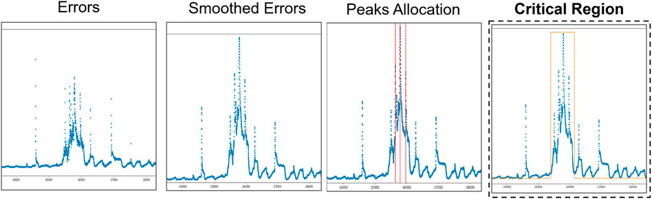
Figure 5. DITAN thresholding methodology.

3.4 Numerical interpretation

The magnitude of scores across sensors within anomalous records can be used to provide sufficient information to allow an understanding and troubleshooting of anomalies. The contribution of each sensor d to an anomalous record i, namely, root-cause, is computed using a softmax function across to its corresponding severity scores s:

$e^{s_d^i}/{\displaystyle \sum _j}{e}^{s_j^i}$

We estimate the similarity between anomalous records in the model-space using the unit dimensionality instead of feature dimensionality. First, we find the internal representations of each record rⁱ. Then, we apply Gaussian Mixture Modeling (GMM) using an optimal number of components to classify each anomalous record to the component with maximum probability p(rⁱ). The anomalous records under the same component are considered similar.

Upon this already validated architecture, we build and introduce here a fifth module (knowledge management), involving physical interpretation of the time series and anomalies. It is a graphical environment which allows to create, read, update and delete (CRUD) knowledge held in the Knowledge Base (KB, see Supplementary Appendix A). The knowledge management module allows complete control over the KB in the form of IF-THEN rules that incorporate temporal constraints or rules. The scope of a rule in our system is to characterize the physical event responsible for the occurrence of a series of conditions.

3.5 DITAN knowledge management module

3.5.1 Conditions

A condition (C) applies to a sensor (S) or physical event (E) that is in an abnormal state. We define five abnormal states: increasing, decreasing, positive, tare and missing values. Although an S-condition can indicate any of these abnormal states, an E-condition can only have a positive abnormal state, meaning that the event has occurred. Therefore, post-condition is always a physical event, while the preconditions consist of one or more S- and/or E-conditions. A condition occurs when an abnormal state is found to be valid for a certain duration. In a given sequence the validation of abnormal states is thus assessed as it follows:

• Increasing: at least three consecutive values exhibit only an increasing trajectory.

• Decreasing: at least three consecutive values exhibit only a decreasing trajectory.

• Positive: consecutive values exhibit only positive values.

• Tare: the first order difference at each step in the sequence results in the same maximum value.

• Missing value: there is at least one missing time-step in the sequence.

3.5.2 Constraints

Following Giannoulis et al. (2019), the preconditions of a rule are constrained using both logical and temporal operators. The conjunction (AND) logical operator is used to combine conditions, while the negation (NOT) logical operator is used to define the abnormal state of a condition. The conditions are temporally constrained such that the start time of the first condition and the start time of the last condition are at most 60 min, 24 h or 7 days apart, introducing lag resolutions of minutes, hours or days across rules. These constraints ensure that all preconditions occur within a defined time interval. The post-condition of a rule exists from the start time of the first condition to the end time of the last condition.

3.5.3 Inference engine

Following Giannoulis et al. (2019), the rule preconditions guide the inference process by incorporating an event-driven protocol, where DITAN’s inference engine is given in Algorithm 1. It is handed the executable rules from the knowledge base (KB) and the anomalous sensor values from critical regions (CR) identified by DITAN in the time series. The objective is to report all post-conditions in the events base (EB), by identifying valid preconditions. This requires support by rule-chains in which the post-condition of a rule lies in the preconditions of another. Thus, in an outer-loop, N executable rules with e events in preconditions are selected from the KB, e being iteratively increased until N becomes zero. At each iteration, the FetchRules function is responsible for selecting and ordering rules. Rules referenced the most frequently are executed first. Given a rule R, RExecute is responsible for validating the occurrences of its conditions across CR (sensor type) or EB (event type). The preconditions of a rule are valid when both temporal and logical constraints are satisfied. The occurrences of a post-condition can also overlap. In such a case, overlapping occurrences are merged. Merging is applied at the end of the algorithm to preserve different event start times which are needed in the chaining process. The final occurrences of R are stored in EB.

Algorithm 1.Inference Engine.

Require: KB, CR ⊳ Knowledge Base (KB), Critical Regions (CR)

Ensure: EB ⊳ Events Base (EB)

  e ← 0 ⊳ Number of events allowed in rule’s precondition

  while True do

     rules ← FetchRules(KB, e) ⊳ Fetch rules ordered by the number of events

     if len(rules) == 0 then ⊳ Halt if there are no more rules

         break

     end if

     for R ∈ rules do

         occurences ← RExecute(CR, EB, R) ⊳ Find occurrences in which R is validated

         if occurences ≠ [] then

              EB.update([R: occurences])⊳ Keep only the executed rules

         end if

     end for

     e + = 1 ⊳ Increase number of events for the next iteration

end while

3.5.4 Rule validation

A rule is valid when its logical and temporal constraints are valid. Validation of the logical constraints (negation, conjunction) is straightforward, because each constraint is a well-defined operator. Instead, further analysis is required for handling temporal relations. Once all valid occurrences of the conditions have been examined, the next step is thus to analyze their temporal differences. To accomplish this, DITAN constructs an upper triangular matrix containing all possible pairs of occurrences for all conditions. For instance, if there are four conditions (C1, C2, C3, C4) DITAN will construct six pairs of categories (C1-C2, C1-C3, C1-C4, C2-C3, C2-C4, C3-C4), and the upper triangular matrix allows consideration of each unique pair of conditions without redundancy. Next, DITAN constructs chains between the occurrences of different pairs so as to derive the final temporal relations. A chain is deemed valid if it incorporates all the different pairs of categories. A pair is added to the chain if it does not violate the temporal constraint. Therefore, a rule is linked to the occurrences of its valid chains (if multiple conditions apply) or its valid condition (if there is only a single condition).

3.5.5 Risk factor

The risk of a (valid) rule is related to the intensity of its preconditions. This is usually quantified by experts using fuzzy logic (Leung and Lam, 1988) or certainty factors (Shortliffe, 1976), such as in Giannoulis et al. (2019). However, DITAN quantifies risk by using the severity scores. The severity score of an anomaly refers to the intensity of its contamination. Local anomalies typically receive lower scores due to their limited impact on the time series as a whole, being primarily confined to a specific region in data. Global anomalies, conversely, tend to receive higher scores, indicating their widespread impact on the time series and significance across multiple data regions. The risk associated with an S condition is equal to the average of the severity scores within the partition (duration) j of a critical region: $R{F}_S=average(C{R}_{\mathit{scores}}^j)$, and the risk of an event E condition is equal to the average risk of its preconditions: RF_E = average(RF_S1, …, RF_Ek). As a result, the risk factor RF provides a general overview of the predictability offset across conditions within their validated durations. The maximum risk is selected when an E condition occurs multiple times within overlapping durations. Finally, to preserve a relative risk across valid rules, within a probabilistic-like range, max-normalization is applied.

3.6 DITAN: initialization of the knowledge management module for Vulcano

DITAN’s “knowledge” is based on rules entered by experts. An example of rule entry via DITAN’s graphical interface is given in Supplementary Appendix B. The time scale of “normal” variations in the time series then needs to be defined, before DITAN is trained and anomalies detected.

3.6.1 Rules

For Vulcano, knowledge is expressed in the form of seven temporal rules R as presented in Table 3. The rules were set to describe severe meteorological (external) events, allowing us to assess storm systems as causes of anomalous decreases in surface temperatures, followed by recovery. We define three event types (Table 3):

1. R1 and R2 define a meteorological event, since only external conditions are linked to each other.

2. R3 to R6 characterize anomalous surface temperature events resulting from external drivers (Figure 3).

3. R7 considers sensor failure, thus finding an “instrumental event.”

Table 3

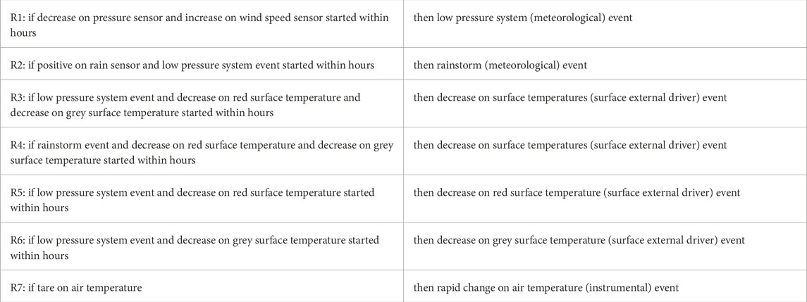
Table 3. The knowledge defined by Experts in the form of temporal rules.

The post-condition of R1 is in the preconditions of R2, R3, R4 and R5, and the post-condition of R2 is in precondition of R4. Instead, R1 and R7 have no events in their preconditions. Therefore, all of the possible inferences are: (a) R1, (b) R1 → R2, (c) R1 → R3, (d) R1 → R2 → R4, (e) R1 → R5, (f) R1 → R6, (g) R7. According to Algorithm 1 executions are divided into three iterations. In the first iteration, (a, g) are executed. In the second iteration, (b, c, e, f) are executed. Finally, in the third iteration, (d) is executed.

3.6.2 Data preparation

There are seven sensors in our Vulcano network (Table 1), for which the frequency of measurements varies between one record every 5 min for the hot and cold stations, and one record per minute for the weather station. Thus, all measurements were sub-sampled to a frequency of 5 min, and then down-sampled (averaged) to a common frequency of one record (time-step) per hour. This results in 6,799 records (for around 283 days), where each record is a vector of seven sensor values. Thus, the temporal resolution of anomalies is expected to be of at least 1 h. An overview of range of values recorded for data set is given in Table 4. There are three main data set characteristics:

1. All temperature sensors exhibit diurnal and annual cycles (normality).

2. Sensors do not have similar value ranges, have scales that differ by six orders of magnitude between rainfall, through temperature, humidity and wind speed, to pressure.

3. There are three significant data gaps in June, September, and October.

Table 4

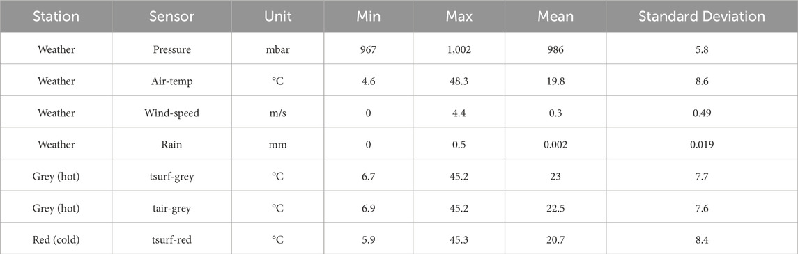
Table 4. Sensor description for Vulcano in the year 2020.

3.6.3 Pre-processing

Of the 1,253 missing time-steps (hours), only 73 can be linearly interpolated. The remaining 1,180 missing time-steps were removed, because they formed gaps that were too long to allow interpolation. Since normality is learned as the regularity of the context-horizon mappings, the impact of these data gaps on the frequency of occurrence of regular context-horizon mappings is negligible due to their relatively small size.

Although decomposition is an option, we chose to decompose measurements solely into the residuals component. This decision was based on the understanding that external phenomena manifest themselves as short-term interruptions to normality causing perturbations to the diurnal cycle. In contrast, the internal driver primarily affects the long-term trend. Therefore, the values of each sensor are transformed into residuals by estimating its decomposition type and period. Min-max normalization is then applied across all sensors to introduce a common scale, without biasing any correlations or underlying distributions. The resulting value range [−3, 3] allows a good spread in range that is not too broad. This ensures that the presence of outlier (extreme) values are not excessively compressed, and maintains outlier relative positions and magnitudes. The effectiveness of the pre-processing strategy is closely tied to its ability to preserve the actual correlations between sensors. The objective is to convert the data into a format suitable for analysis and input into DITAN, while still preserving the inherent relationships within the data. A summary of pre-processing output is given in Table 5.

Table 5

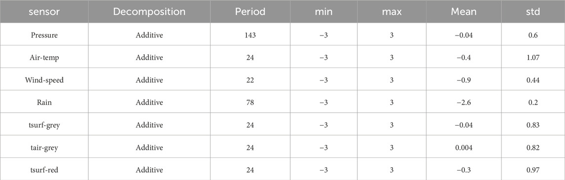
Table 5. Pre-processed sensor description for Vulcano in the year 2020.

3.6.4 Forecasting scenario

The selection of the appropriate size for observation context and forecast horizon needs to be based on the time scale of expected variations. Surface temperatures will exhibit diurnal cycles of 24 h, while also following an annual cycle. In addition, following (Sanders, 1984) major storm systems will develop over hours so that parameters such as wind speed and pressure will evolve over timescales of 6–24 h during high intensity events, such as Medicanes. Thus, following Haque et al. (2021) the context window is set to 24 h to allow a forecast horizon of 6 h.

The training phase of DITAN is thus conducted on data with 24 h context size and 6 h horizon size. The aim of learning is to reduce the differences between forecasted and actual values by identifying suitable model parameters. To ensure equal importance in minimizing all differences, we employ mean absolute error (MAE) as the loss function. By using absolute differences to compute gradients of the loss function, DITAN can mitigate the influence of extreme events such as Mediterranean hurricanes, which would otherwise dominate as the main indicator of normality. Instead, DITAN prioritizes the average understanding of underlying patterns, with patterns appearing more frequently having a greater influence on determining normality.

During the Bayes optimization process, a total of 20 different hyper-parameter configurations were examined. Each configuration was assessed using four expanding time windows applied to the pre-processed data set, resulting into an examination of 80 (=4 × 20) models. The first (initial) configuration is described in Table 6.

Table 6

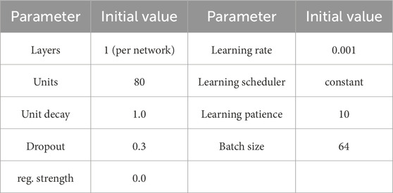
Table 6. Initial parameter setup.

We observe that no improvement occurs until the 5^th configuration, with a significant improvement being observed during the 6^th configuration with relatively small variations occurring up to the 16th configuration. A gradual decrease is then observed between the 16th and 20th configurations, at which point the objective function converges (Figure 6). By changing from the initial to the optimal configuration, the optimization error is decreased from 0.268 to 0.195, resulting in a 27% improvement on the objective function.

Figure 6

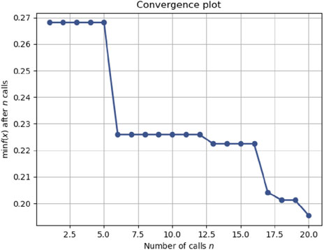
Figure 6. Convergence plot of DITAN across configurations using Bayes Optimizer.

The hyper-parameters of the optimal (20th) configuration are reported in Table 7. The resulting model consists of 19.815 parameters. These parameters are updated in batches of 32 consecutive patterns, where each record within these patterns is encoded using 32 units. In addition, use of a larger learning rate of 0.01 means that the convergence process becomes capable at exploring global maxima more effectively throughout all epochs. To maintain stability during training, a step decay factor is used, which gradually reduces the learning rate every 4 epochs. This approach strikes a balance between exploration and stability in the optimization process. The final parameters are selected at epoch 78, at which point the patience of early stopping is exhausted, with the internal validation loss not improving by $>0.0003$ for 10 consecutive epochs after epoch 68.

Table 7

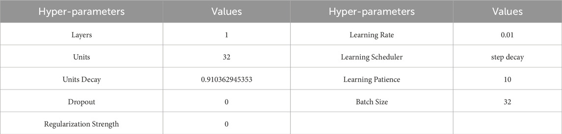
Table 7. The hyper-parameters of the optimal DITAN model.

3.6.5 Detecting anomalies

In the detection phase the trained model is used to predict normality across 6,843 (records) hours, resulting in a corresponding number of errors per sensor, as illustrated in Figure 7. Each error is computed as the absolute difference between the predicted and observed value, according to the selected loss function. Each sequence is then smoothed using a simple moving average (SMA) of 6-hour. An important consideration when reducing temporal resolution is to maintain a balanced trade-off between smoothness and introduced lag. The “goodness” of the proposed window size is demonstrated in Figure 8, using a subset of errors from a randomly selected (pressure) sensor. We observe that the smoothed versions of the errors maintain a responsiveness to the raw errors.

Figure 7

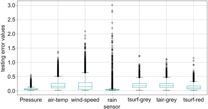
Figure 7. Box plots of the prediction errors of DITAN across the 7 sensors. For each sensor, the boxplot consists of a rectangular box which spans the interquartile range (IQR) of the data, the line inside representing the median. “Whiskers” extend from the edges of the box to indicate the range of the data outside the IQR, often with outliers (black points) shown beyond the whiskers. Small median errors were observed for all sensors with small IQRs. Several outliers were observed for the rain sensor, since rain is a rare event in the observed sequence.

Figure 8

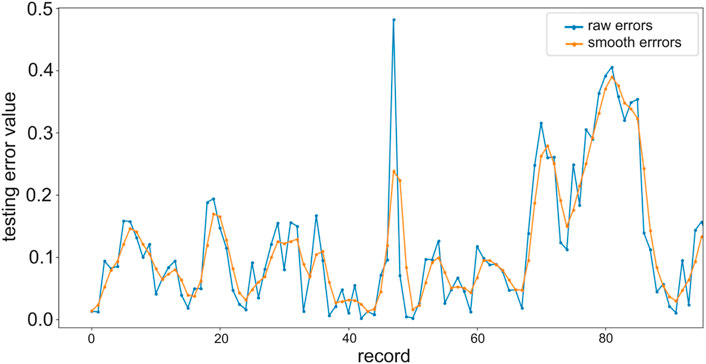
Figure 8. A sub-part of the raw and smoothed error sequences on pressure sensor.

4 Results

Our objective is to examine the intensity, duration and type of anomalies caused on surface temperature by meteorological/atmospheric effects at a hydrothermal system. External drivers on the thermal state of the surface are described by air pressure, wind speed, rain, humidity and air temperature. To do this, DITAN detects anomalies across the seven sensors, and then uses the expert rules to interpret them as physical events. Within this framework, two or more anomalies are considered to be linked to each other when their start difference is within a defined time interval.

4.1 Normality

Figure 9 gives key statistics of the preprocessed sensors. We see 3 features of normality: one typical of the meteorological system, and two characteristic of the hydrothermal system:

1. The four sensors of the meteorological station recording the external parameters (pressure, air temperature, wind-speed, and rain), exhibit the expected correlation during the passage of a low-pressure system. That is, as pressure falls so too does air temperature, but wind speed and rainfall increase.

2. The surface temperatures for the hot zone exhibit a higher median than those of the cold zone. This is because the surface temperature of the hot zone is buffered by the enhanced geothermal heat flux associated with the hydrothermal system. The difference between the medians for the two surface temperatures (0.3) thus gives the median normalized magnitude of ΔT for the year 2020.

3. The median air temperature in the hot zone is higher than that at the weather station, again due to buffering by the geothermally heated surface 15 cm below the air temperature sensor, giving a median normalized magnitude for the air temperature anomaly during 2020 of 0.5.

Figure 9

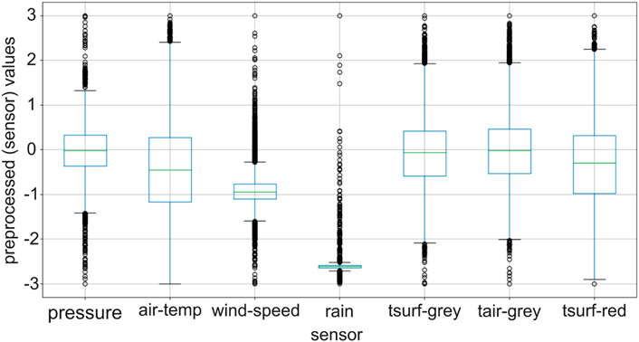
Figure 9. Box-plot of the pre-processed data for Vulcano in 2020. Despite the fact that decomposing to only residuals results in more values outside of the interquartile ranges, the sensors are able to preserve their correlations.

4.2 Anomalies

From the 6,843 records (hours), 1,737 were detected as anomalous. This means around 72 days (or 25% of total records) experience anomalous events. The number of anomalies and critical regions per sensor are given in Table 8. The most critical regions occur on the temperature sensors, but the number of critical regions in the cold zone is slightly higher than in hot zone for air and surface temperatures. This again highlights the buffering effect of the geothermal heat flux in the hot zone. Wind-speed, rain and pressure also exhibit anomalies, indicating that the main source of anomalies on the temperature sensors at Vulcano during 2020, and thus also on ΔT, were due to external drivers.

Table 8

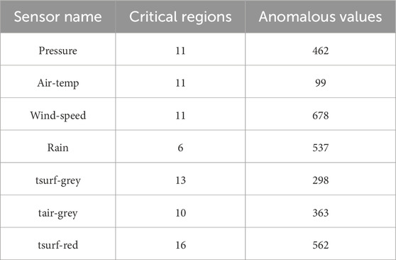
Table 8. DITAN’s detection results per sensor.

4.3 Rule execution

The number of valid executions per rule are given in Table 9. The two meteorological events (rules R1 and R2) are executed seven and three times, respectively. Instead, R4 does not occur, R3 and R6 are executed only once, and R5 twice. This highlights the influence of external drivers on the surface temperature on both the hot and cold zones, but with a higher influence on the cold zone. Rule R7 was executed nine times. This indicates that data were corrupted on nine occasions due to the sensor giving a spurious output, such as during automatic reset, or the presence of recording glitches.

Table 9

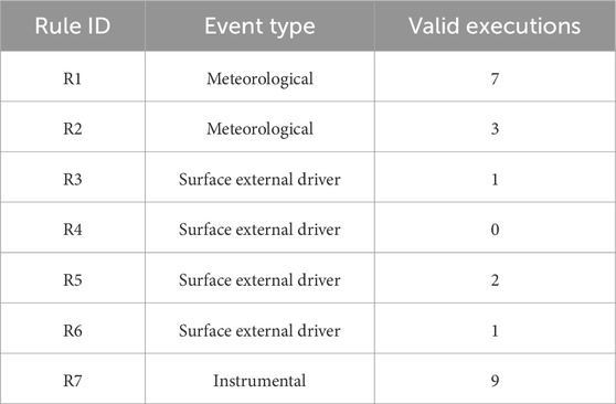
Table 9. Rules executed using the inference engine.

The main anomalous meteorological events occurring at Vulcano in the year 2020 were thus associated with the passage of low pressure systems and rainstorms (cloudbursts), as defined by rules R1 and R2, respectively. To obtain the temporal occurrences of these anomalous meteorological events we need to analyze the critical regions of DITAN within the pressure, rain and wind speed sensors, where the root-causes of the critical regions in these sensors are given in Figure 10. Recall that root causes are probabilistic contributions of each sensor to the anomalous character of a time-step (record), ranging from 0 to 1. During normal time-steps, all root cause values are set to zero. Consequently, the root cause diagrams provides a detailed analysis, at a time-step resolution, of the temporal difference (delay) between anomalous events triggered at various sensors. We observe that most of critical regions for wind speed and pressure are closely correlated in terms of time, contributing to the occurrence of R1. The critical regions for rain are concentrated later in the year, in close proximity to critical regions for wind speed and pressure, resulting in execution of R2 at this time.

Figure 10

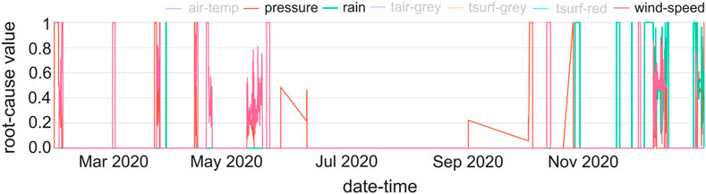
Figure 10. The root-causes diagram for pressure, rain and wind speed sensors.

4.4 Abnormal meteorological events

Critical regions for the air pressure sensor demonstrate a negative correlation with the wind speed sensor. This implies that when pressure exhibits an abnormal decrease, the anomalous values of the corresponding critical region for wind speed tends to increase. The positive correlation with critical regions of the rain sensor indicate that low pressure systems that were classified as abnormal were also associated with intense rain fall. We here use abnormal in the sense that the pressure, wind speed and rainfall intensity associated with the low pressure system in question was not normal compared with the trends learnt by DITAN for “regular” system behavior.

Of all the 19 critical regions identified for 2020, nine are for pressure, seven are for wind speed, and two are for rain. Abnormalities in the time series for pressure, wind speed and rainfall, related to passage of a low pressure system (Rule R1), occurred during the first 4 months of 2020, and then again in December. R1 was executed (Figure 11):

• once in early-February (event duration = 2 days);

• once in late-March (event duration = 2 days);

• once in mid-April (event duration = 1 day);

• once in early-May (event duration = 5 days);

• three times during December (combined duration = 4 days).

Figure 11

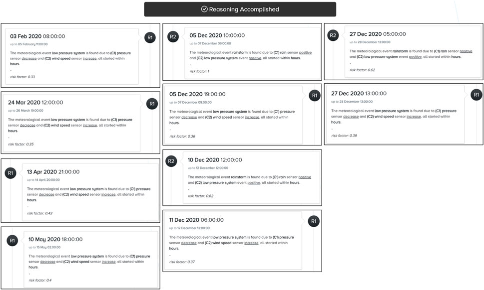
Figure 11. Timeline of detected meteorological events (R1, R2).

Summer and autumn lacked abnormal meteorological events, with all sensors maintaining relatively low (normal) levels (Figure 11). Rainfall remained at relatively low (normal) levels during the spring, summer and autumn months of 2020, but in December the rainstorm rule (R2) was executed three times. These abnormal rainstorm events lasted a total of 5 days, and coincided with the three occurrences of abnormalities due to low pressure systems.

4.5 Abnormalities in surface temperatures

The values of the surface temperatures in both the cold and hot zones are positively correlated (Figure 12). However, a partial correlation is observed between their anomalous values within critical regions, since the surface temperature of the hot zone is buffered to the external conditions by the internal driver (i.e., the geothermal heat source). Two critical regions were identified for surface temperature in both the hot zone and cold zone (Figure 13). Anomalies are confined to the winter and spring months, while summer and autumn are free of critical regions. An abnormal decrease in surface temperature in the cold zone (R5) was detected in early-February and lasted 2 days, although this did not affect the hot zone. An abnormal decrease in surface temperature was recorded for both zones in mid-May, and lasted 6 days. During this period, the surface temperature at the hot zone began to decrease a few hours before the cold zone.

Figure 12

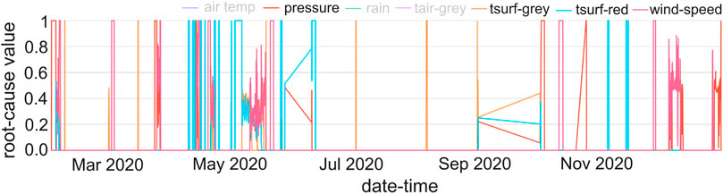
Figure 12. The root-causes diagram for pressure, wind speed and (red, grey) surface temperature sensors.

Figure 13

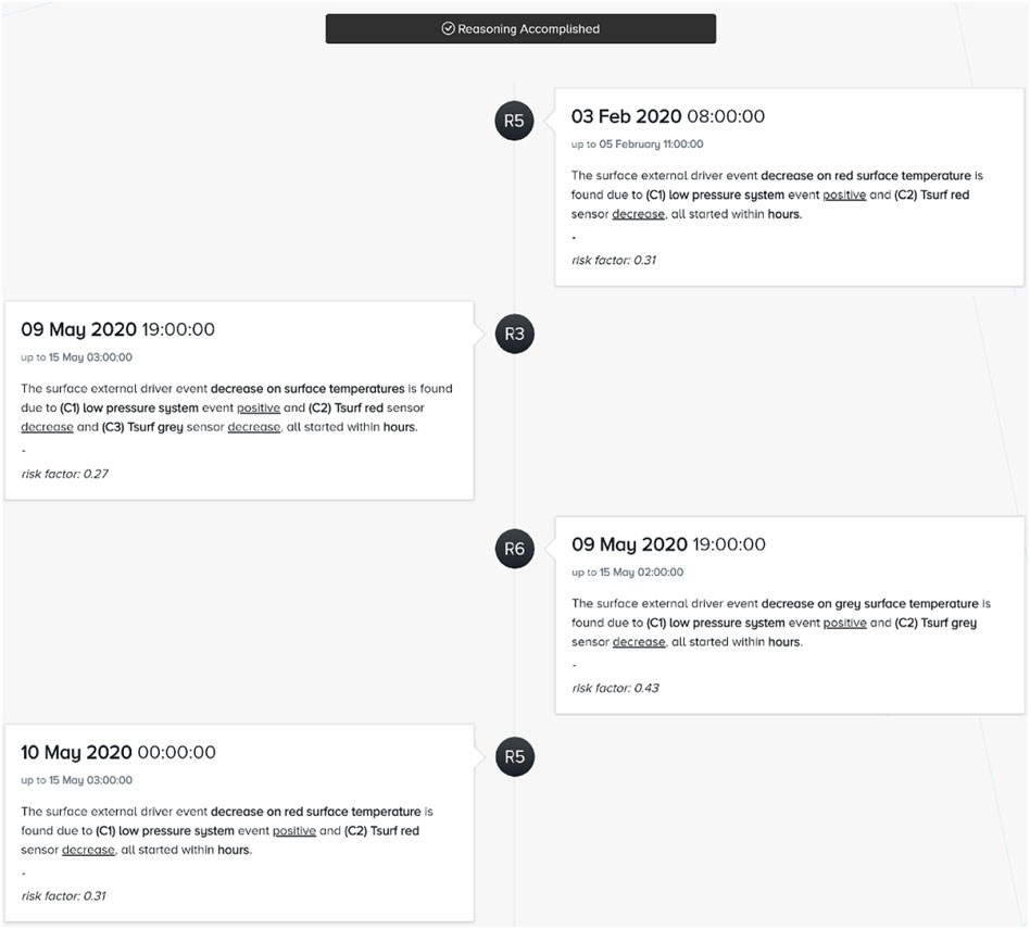
Figure 13. The timeline of the detected surface external driver events (R3, R5, R6).

The two-day-long February abnormality in surface temperature began on 3 February, and was characterized by a dampening of the diurnal cycle, but only for the cold zone whose amplitude decreased by 4°C (Supplementary Appendix C). Abnormality began around midnight of 2–3 February, and was coincident with an abnormal decrease in pressure from 996 mbar to 976 mbar until midnight on 4–5 February. The pressure drop at 0.4 mb h^-1 was matched by an increase in wind speed from 7 km/h to 36 km/h, with no rainfall being recorded (Supplementary Appendix C). DITAN therefore characterized this meteorological event as a low-pressure system, but not a rain storm.

The six-day-long May surface temperature abnormality began on 9 May, continued until 15 May, and affected both the cold and the hot zones. The abnormality was due to a dampening of the diurnal cycles in surface temperature by 2°C–3°C (Supplementary Appendix C). For the 6 days prior to the abnormality diurnal ranges were 10°C (32°C–22°C) in the cold zone and 16°C (36°C–20°C) in the hot zone, whereas for the 6 days of abnormality ranges were 8°C (32°C–26°C) and 13°C (31°C–18°C). The surface temperature abnormality was associated with an abnormality in pressure which fell from 990 mbar to 976 mbar over 48 h beginning at midnight 8–9 May (Supplementary Appendix C). Pressure recovered on 15–16 May, also synchronous with the end of abnormality in surface temperature. The greatest decrease in pressure was at a rate of 1 mbar per hour during 10 May, which classes the event as a “meteorological bomb.” Such events are defined as “extra-tropical surface cyclones whose central pressure fall averages at least 1 mbar h^-1 for 24 h” being a “maritime, cold-season event, with hurricane-like features” (Sanders and Gyakum, 1980). Meteorological bombs are not necessarily associated with rain, but are associated with sustained high winds which increase as the pressure decreases, making them “wind storms” (Sanders and Gyakum, 1980). Indeed, the 6 days of abnormality were characterized by no rain, but winds peaked at 30 km/h which was twice the speed recorded in the 6 days prior to passage of the bomb (Supplementary Appendix C) and, given the sheltered location of the anemometer inside the crater, high. DITAN therefore also characterized this event as an anomalous low-pressure system, but not a rain storm.

Surface temperature abnormalities are thus due to suppressed ranges of the diurnal cycle. This is triggered by decreases in pressure, which would have increased radiative cooling of the surface through its influence on vapor pressure. In addition, forced convection would have been greatly enhanced by the high winds. The combined effect is to dampen the diurnal cycle of surface temperature, making the cycles abnormal.

4.6 Prediction errors

Figure 7 presents the prediction errors across sensors, and based on these errors, the risk associated with the occurrence of abnormal meteorological events is also depicted in Figure 11. The risk of an abnormal low-pressure system varies from 0.33 to 0.43, whereas the risk of an abnormal rainstorm varies from 0.62 to the maximum risk of 1.0. That is because, especially during the early days of December, the prediction offset in rain activity was higher than the prediction offset of wind speed and pressure activities.

The risk of abnormal decrease in cold surface temperature (R5) is 0.31, while the risk of abnormal decrease of hot surface temperature (R6) is higher at 0.43 (Figure 13). This suggests that abnormal surface temperature changes in the hot zone have a higher level of risk of occurrence than in the cold zone. In addition, the risk of abnormal surface temperature decreases at both cold and hot zones (R3) is 0.27, which is lower because it considers all conditions from R5 and R6. This observation suggests that abnormal temperature changes across the entire surface carry slightly less risk of occurrence compared to changes in either the cold zone or hot zone temperatures.

5 Discussion

The critical regions for surface temperatures in the cold and hot zones, as well as wind speed and pressure, are given as a root-causes diagram in Figure 12. The detected physical events associated with anomalies in these critical regions have been checked as true positives (Table 10). This analysis shows that critical regions for surface temperature, wind speed and pressure are closely associated, showing partial or complete overlap. The passage of abnormally intense low pressure systems (meteorological event R1) always caused surface temperature anomalies involving abnormal decreases in temperature. Meteorological event R1 drove decreases in surface temperature for both hot and cold zones. However, the cooling experienced by the hot zone was modulated by the effect of the hydrothermal system heat source. Thus, critical regions were more associated with passage of a low pressure system for the cold zone than the hot zone.

Table 10

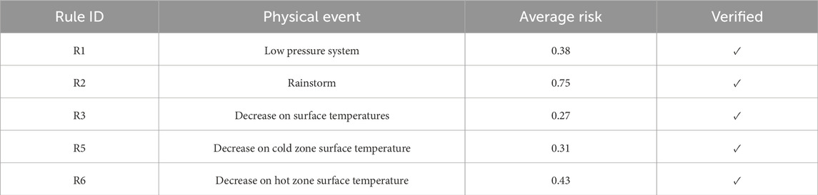
Table 10. The detected meteorological and surface external driver events.

This has implications for the effect of external drivers on the surface thermal anomaly (ΔT). In early-February 2020, a low-pressure system passed over Vulcano, persisting for 2 days. During this period, the cold zone experienced an abnormal decrease in surface temperature. However, no abnormality was recorded in the hot zone. This, thus, drove the thermal anomaly upwards, but increasing ΔT was the result of an external rather than an internal driver. However, the effect was limited to just 2 days. A second low pressure system passed over Vulcano in late-March and lasted 2 days. This was followed a one day-long period of low pressure system conditions in mid-April. In both of these cases, there were no abnormalities in the surface temperatures at either the cold or hot zones, meaning that the thermal anomaly was unaffected. However, in early-May, a low-pressure system persisted for approximately 5 days. Its influence decreased the surface temperature in the hot zone and the cold zone, disrupting normality across the entire surface. Abnormal rainstorm events were detected throughout December, and were associated with abnormalities in wind speed and pressure. However, surface temperatures retained their normality in both the cold and hot zones.

This means that, even when at low, baseline levels, external drivers have a minimal role in causing abnormalities in surface temperature in the hot and cold zones, and hence also the surface thermal anomaly. Passage of intense low pressure systems with high winds was the main external driver for abnormal variations in surface temperature. However, even the most intense, cloudburst events did not force abnormality on the surface temperature time series, meaning that when the system is at baseline levels, surface temperature normality is immune to rain. However, this conclusion applies only to surface temperatures (Pailot-Bonnétat et al., 2023; Pailot-Bonnétat and Harris, 2024).

5.1 Physical link between intensity of meteorological abnormality and surface cooling

At Vulcano, heat produced by condensation of ascending hydrothermal fluids has been shown to heat the surface (Chiodini et al., 2005) buffering the surface temperature so that surfaces are warmer than in an ambient scenario. Both heated and non-heated surfaces undergo diurnal and annual variation. Thus, because the heated surface is just a few degrees greater than ambient it is subject to the same external factors, such as solar heating, wind and rain, that drive surface heating and cooling. However, temperature cycles for the heated zone are at a higher level, thus creating the thermal anomaly (ΔT). For 2020 at Vulcano we found that the only external factor that could drive an abnormal behavior in the diurnal cycles was particularly low atmospheric pressures and wind speeds, rain not playing a role.

5.2 Abnormality in the thermal anomaly due to external drivers

Only particularly intense and long lasting low-pressure systems associated with meteorological bombs can dampen the diurnal cycles at both heated and non-heated surfaces. In such a case, because both T_h and T₀ behave in the same way, there is no abnormality in ΔT. However, passage of less intense systems of shorter duration only dampen the cycles in T₀, thereby causing abnormality in ΔT. The buffering provided by the internal heat source is sufficient to protect the hot surface from abnormal cooling. Thus, we consider passage of moderate intensity systems the only external driver on ΔT, where the effect of abnormal decrease in T₀, but not T_h, will increase ΔT for the period of the event.

6 Conclusion

Deep learning is beginning to be applied to understand abnormalities in diurnal cycles of surface temperature in non-volcanic environments, such as at urban heat islands (Qi et al., 2023), but not yet at low temperature thermal anomalies associated with hydrothermal systems. At bottom-heated surfaces above hydrothermal systems, due to the low amplitude of the anomaly we expect the form and amplitude of diurnal cycles in surface temperature to have both external drivers (the meteorological system) and internal drivers (the magmatic and hydrothermal systems). However, the role of the meteorological system in driving abnormality in surface temperatures at both geothermally heated and non-heated ground, in a vegetation-free crater, is poorly constrained. Most studies focus instead on the role of rainfall in influencing meteoric inflow into the hydrothermal mixing zone (Carapezza et al., 1981; Chiodini et al., 1995; Nuccio et al., 1999). We have thus applied DITAN to a year of meteorological data for the geothermally-heated zone in the Vulcano Fossa crater to understand the role of external (meteorological) factors in heating and cooling the surface.

We intentionally chose the year 2020, as heat fluxes were particularly low and stable allowing us to assess the background state of the system. Defining baselines is fundamental in volcano surveillance (McGuire et al., 1995). In the baseline state, the system appears to be remarkably robust and relatively immune to external drivers. Divergence from normality in surface temperature only occurred twice, and was associated with the passage of particularly intense low-pressure systems with durations of 2–5 days. Abnormal rainfall events did not cause divergence from normality in surface temperature cycles. Thus, during low levels of heat flux, external factors play a minimal role in driving the system away from normality in terms of diurnal and seasonal cycles of surface heating and cooling.

When applied to meteorological and surface temperature time series for surfaces above an active hydrothermal system, and configured with rules to define physical events, DITAN allows anomalies driven by external factors to be detected and classified. It could thus be applied to any geothermal system where appropriate data are available. If, as here, applied during a period when external drivers are variable, but internal drivers are stable and at background levels, all anomalies will be characteristic of a “stable” system whose surface temperature abnormalities are only driven by meteorological events. Once this is defined, such externally-driven abnormalities can be identified, cleaned and removed from periods when the internal drivers become variable and, hence, the hydrothermal system becomes unstable.

We consider this work as test and starting point for a model that cleans data set of externally driven thermal anomalies, isolating abnormalities in thermal anomalies due to internal drivers, such as recharge of the magmatic system or changes in system permeability. During our period of study, no such events occurred. However, recharge of the magmatic system or changes in system permeability can be the prelude to eruption, or enhanced CO₂ soil degassing, so that isolating such internal changes is fundamental. That the thermal anomaly is so subtle, and that influences on it are multivariate, makes this task challenging, and hence requiring of a machine-learning based approach. Thus, defining the key internal drivers for, and their association and temporal interplay with, surface temperature abnormalities as the system moves into unrest will be our next step.

Data availability statement

The raw data supporting the conclusion of this article will be made available by the authors, without undue reservation.

Author contributions

MG: Conceptualization, Methodology, Software, Writing–original draft, Writing–review and editing, Investigation. SP-B: Data curation, Resources, Validation, Writing–original draft, Writing–review and editing, Investigation. VB: Conceptualization, Formal Analysis, Supervision, Writing–original draft, Writing–review and editing. AH: Data curation, Funding acquisition, Supervision, Validation, Writing–original draft, Writing–review and editing, Conceptualization.

Funding

The authors declare that financial support was received for the research, authorship, and/or publication of this article. ANR-19-CE04-0014-01 DIRE.

Conflict of interest

The authors declare that the research was conducted in the absence of any commercial or financial relationships that could be construed as a potential conflict of interest.

Publisher’s note

All claims expressed in this article are solely those of the authors and do not necessarily represent those of their affiliated organizations, or those of the publisher, the editors and the reviewers. Any product that may be evaluated in this article, or claim that may be made by its manufacturer, is not guaranteed or endorsed by the publisher.

Supplementary material

The Supplementary Material for this article can be found online at: https://www.frontiersin.org/articles/10.3389/feart.2024.1372621/full#supplementary-material

References

Alparone, S., Cannata, A., Gambino, S., Gresta, S., Milluzzo, V., and Montalto, P. (2010). Time-space variation of volcano-seismic events at La Fossa (Vulcano, Aeolian Islands, Italy): new insights into seismic sources in a hydrothermal system. Bull. Of Volcanol. 72, 803–816. doi:10.1007/s00445-010-0367-6

CrossRef Full Text | Google Scholar

Aubert, M., Diliberto, S., Finizola, A., and Chébli, Y. (2008). Double origin of hydrothermal convective flux variations in the Fossa of Vulcano (Italy). Bull. Of Volcanol. 70, 743–751. doi:10.1007/s00445-007-0165-y

CrossRef Full Text | Google Scholar

Bahrami, A., Safavinejad, A., and Amiri, H. (2019). Spectral radiative entropy generation in a non-gray planar participating medium including H2O and CO2. J. Of Quantitative Spectrosc. And Radiat. Transf. 227, 32–46. doi:10.1016/j.jqsrt.2019.01.024

CrossRef Full Text | Google Scholar

Bonneville, A., and Gouze, P. (1992). Thermal survey of Mount Etna volcano from space. Geophys. Res. Lett. 19, 725–728. doi:10.1029/92gl00580

CrossRef Full Text | Google Scholar

Carapezza, M., Nuccio, P., and Valenza, M. (1981). Genesis and evolution of the fumaroles of Vulcano (Aeolian Islands, Italy): a geochemical model. Bull. Volcanol. 44, 547–563. doi:10.1007/bf02600585

CrossRef Full Text | Google Scholar

Carniel, R., and Guzmán, S. (2020). Chapter machine learning in volcanology: a review. London, UK: InTechOpen.

Google Scholar

Chiodini, G., Cioni, R., Marini, L., and Panichi, C. (1995). Origin of the fumarolic fluids of Vulcano Island, Italy and implications for volcanic surveillance. Bull. Of Volcanol. 57, 99–110. doi:10.1007/bf00301400

CrossRef Full Text | Google Scholar

Chiodini, G., Granieri, D., Avino, R., Caliro, S., Costa, A., and Werner, C. (2005). Carbon dioxide diffuse degassing and estimation of heat release from volcanic and hydrothermal systems. J. Of Geophys. Res. Solid Earth 110. doi:10.1029/2004jb003542

CrossRef Full Text | Google Scholar

Corradino, C., Ramsey, M., Pailot-Bonnétat, S., Harris, A., and Del Negro, C. (2023). Detection of subtle thermal anomalies: deep learning applied to the ASTER global volcano dataset. IEEE Trans. Geoscience And Remote Sens. 61, 1–15. doi:10.1109/tgrs.2023.3241085

CrossRef Full Text | Google Scholar

Diliberto, I. (2011). Long-term variations of fumarole temperatures on Vulcano Island (Italy). Ann. Of Geophys.

Google Scholar

Dobson, P., Kneafsey, T., Hulen, J., and Simmons, A. (2003). Porosity, permeability, and fluid flow in the Yellowstone geothermal system, Wyoming. J. Of Volcanol. And Geotherm. Res. 123, 313–324. doi:10.1016/s0377-0273(03)00039-8

CrossRef Full Text | Google Scholar

Ferreira, A., Curilem, M., Gomez, W., and Rios, R. (2023). Deep learning and multi-station classification of volcano-seismic events of the Nevados del Chillán volcanic complex (Chile). Neural Comput. And Appl. 35, 24859–24876. doi:10.1007/s00521-023-08994-z

CrossRef Full Text | Google Scholar

Ferrucci, F., Gaudiosi, G., Milano, G., and Nercessian, A. (1991). Seismological exploration of Vulcano (aeolian islands): case history. Acta Vulcanol.

Google Scholar

Giannoulis, M., Harris, A., and Barra, V. (2023). DITAN: a deep-learning domain agnostic framework for detection and interpretation of temporally-based multivariate ANomalies. Pattern Recognit. 143, 109814. doi:10.1016/j.patcog.2023.109814

CrossRef Full Text | Google Scholar

Giannoulis, M., Kondylakis, H., and Marakakis, E. (2019). Designing and implementing a collaborative health knowledge system. Expert Syst. Appl. 126, 277–294. doi:10.1016/j.eswa.2019.02.010

CrossRef Full Text | Google Scholar

Haque, E., Tabassum, S., and Hossain, E. (2021). A comparative analysis of deep neural networks for hourly temperature forecasting. IEEE Access 9, 160646–160660. doi:10.1109/access.2021.3131533

CrossRef Full Text | Google Scholar

Harris, A. (2013). Thermal remote sensing of active volcanoes: a user’s manual. Cambridge, England: Cambridge University Press.

Google Scholar

Harris, A., Alparone, S., Bonforte, A., Dehn, J., Gambino, S., Lodato, L., et al. (2012). Vent temperature trends at the Vulcano Fossa fumarole field: the role of permeability. Bull. Of Volcanol. 74, 1293–1311. doi:10.1007/s00445-012-0593-1

CrossRef Full Text | Google Scholar

Harris, A., Lodato, L., Dehn, J., and Spampinato, L. (2009). Thermal characterization of the Vulcano fumarole field. Bull. Of Volcanol. 71, 441–458. doi:10.1007/s00445-008-0236-8

CrossRef Full Text | Google Scholar

Harris, A., and Stevenson, D. (1997). Thermal observations of degassing open conduits and fumaroles at Stromboli and Vulcano using remotely sensed data. J. Of Volcanol. And Geotherm. Res. 76, 175–198. doi:10.1016/s0377-0273(96)00097-2

CrossRef Full Text | Google Scholar

Hochreiter, S., and Schmidhuber, J. (1997). Long short-term memory. Neural Comput. 8, 1735–1780. doi:10.1162/neco.1997.9.8.1735

PubMed Abstract | CrossRef Full Text | Google Scholar

Hochstein, M. (2005). “Heat transfer by hydrothermal systems in the east african rifts,” in Proceedings Of The World Geothermal Congress 2005, Antalya, Turkey.

Google Scholar

Hochstein, M., and Browne, P. (2000). Surface manifestations of geothermal systems with volcanic heat sources. Encycl. Of Volcanoes, 835–855.

Google Scholar

Ishibashi, H., Tomabechi, R., Nishidate, K., Osaka, N., Shimomura, T., Yamada, S., et al. (2023). Evaluation of radiative absorption effect to estimate mean radiant temperature in environments with high water vapor concentration such as in a sauna. Build. And Environ. 243, 110684. doi:10.1016/j.buildenv.2023.110684

CrossRef Full Text | Google Scholar

Keszthelyi, L., Harris, A., and Dehn, J. (2003). Observations of the effect of wind on the cooling of active lava flows. Geophys. Res. Lett. 30. doi:10.1029/2003gl017994

CrossRef Full Text | Google Scholar

Lagios, E., Vassilopoulou, S., Sakkas, V., Dietrich, V., Damiata, B., and Ganas, A. (2007). Testing satellite and ground thermal imaging of low-temperature fumarolic fields: the dormant Nisyros Volcano (Greece). ISPRS J. Of Photogrammetry And Remote Sens. 62, 447–460. doi:10.1016/j.isprsjprs.2007.07.003

CrossRef Full Text | Google Scholar

Leung, K., and Lam, W. (1988). Fuzzy concepts in expert systems. Computer. 21, 43–56. doi:10.1109/2.14346

CrossRef Full Text | Google Scholar

Luong, T., Pham, H., and Manning, C. D. (2015). “Effective approaches to attention-based neural machine translation,” in Proc. of the 2015 Conf. on Empirical Methods in Natural Language Processing, Lisbon, Portugal, September 17-21, 2015, 1412–2142. doi:10.18653/v1/d15-1166

CrossRef Full Text | Google Scholar

Malfante, M., Dalla Mura, M., Mars, J., Métaxian, J., Macedo, O., and Inza, A. (2018). Automatic classification of volcano seismic signatures. J. Of Geophys. Res. Solid Earth 123, 10–645. doi:10.1029/2018jb015470

CrossRef Full Text | Google Scholar

Manley, G., Mather, T., Pyle, D., Clifton, D., Rodgers, M., Thompson, G., et al. (2022). A deep active learning approach to the automatic classification of volcano-seismic events. Front. Earth Sci. 10, 807926. doi:10.3389/feart.2022.807926

CrossRef Full Text | Google Scholar

Mannini, S., Harris, A., Jessop, D., Chevrel, M., and Ramsey, M. (2019). Combining ground-and ASTER-based thermal Measurements to Constrain fumarole field heat budgets: the case of Vulcano Fossa 2000–2019. Geophys. Res. Lett. 46, 11868–11877. doi:10.1029/2019gl084013

CrossRef Full Text | Google Scholar

B. McGuire, C. Kilburn, and J. Murray (1995). Monitoring active volcanoes: strategies, procedures and techniques. 1st ed. (England, UK: Routledge).

Google Scholar

Nicholson, K., and Nicholson, K. (1993). Geothermal systems. Geotherm. Fluids Chem. And Explor. Tech., 1–18. doi:10.1007/978-3-642-77844-5_1

CrossRef Full Text | Google Scholar

Nuccio, P., Paonita, A., and Sortino, F. (1999). Geochemical modeling of mixing between magmatic and hydrothermal gases: the case of Vulcano Island, Italy. Earth And Planet. Sci. Lett. 167, 321–333. doi:10.1016/s0012-821x(99)00037-0

CrossRef Full Text | Google Scholar

Pailot-Bonnétat, S., and Harris, A. (2024). A thermal record for unrest at Vulcano 2020–2022: in situ meteorological data and soil temperature recorded at high temporal resolution. Bull. Of Volcanol. 86, 13. doi:10.1007/s00445-023-01696-3

CrossRef Full Text | Google Scholar

Pailot-Bonnétat, S., Rafflin, V., Harris, A., Diliberto, I., Ganci, G., Cappello, A., et al. (2023). Others Anatomy of thermal unrest at a hydrothermal system: case study of the 2021-2022 crisis at Vulcano.

Google Scholar

Qi, W. Q., Wang, X., Meng, Y., Zhou, Y., and Wang, H. (2023). Exploring the impact of urban features on the spatial variation of land surface temperature within the diurnal cycle. Sustain. Cities Soc. 91, 104432. doi:10.1016/j.scs.2023.104432

CrossRef Full Text | Google Scholar

Sanders, F. (1984). The meteorological ”bomb”; an explosive maritime cyclone. OCEANS 1984 318-323.

Google Scholar

Sanders, F., and Gyakum, J. (1980). Synoptic-dynamic climatology of the bomb. Mon. Weather Rev. 108, 1589–1606. doi:10.1175/1520-0493(1980)108<1589:sdcot>2.0.co;2

CrossRef Full Text | Google Scholar

Sekioka, M., and Yuhara, K. (1974). Heat flux estimation in geothermal areas based on the heat balance of the ground surface. J. Of Geophys. Res. 79, 2053–2058. doi:10.1029/jb079i014p02053

CrossRef Full Text | Google Scholar

Shortliffe, E. (1976). Books: computer-based medical consultations: MYCIN. J. Of Clin. Eng. 1, 69. doi:10.1097/00004669-197610000-00011

CrossRef Full Text | Google Scholar

Stimac, J., Goff, F., and Goff, C. (2015). Intrusion-related geothermal systems. Encycl. Of Volcanoes, 799–822. doi:10.1016/b978-0-12-385938-9.00046-8

CrossRef Full Text | Google Scholar

Watson, A., Schuster, U., Shutler, J., Holding, T., Ashton, I., Landschützer, P., et al. (2020). Revised estimates of ocean-atmosphere CO2 flux are consistent with ocean carbon inventory. Nat. Commun. 11, 4422. doi:10.1038/s41467-020-18203-3

PubMed Abstract | CrossRef Full Text | Google Scholar

White, D., Muffler, L., and Truesdell, A. (1971). Vapor-dominated hydrothermal systems compared with hot-water systems. Econ. Geol. 66, 75–97. doi:10.2113/gsecongeo.66.1.75

CrossRef Full Text | Google Scholar