Determining the Moho topography using an improved inversion algorithm: a case study from the South China Sea

The Parker-Oldenburg method, as a classical frequency-domain algorithm, has been widely used in Moho topographic inversion. The method has two indispensable hyperparameters, which are the Moho density contrast and the average Moho depth. Accurate hyperparameters are important prerequisites for inversion of fine Moho topography. However, limited by the nonlinear terms, the hyperparameters estimated by previous methods have obvious deviations. For this reason, this paper proposes a new method to improve the existing Parker-Oldenburg method by taking advantage of the invasive weed optimization algorithm in estimating hyperparameters. The synthetic test results of the new method show that, compared with the trial and error method and the linear regression method, the new method estimates the hyperparameters more accurately, and the computational efficiency performs excellently, which lays the foundation for the inversion of more accurate Moho topography. In practice, the method is applied to the Moho topographic inversion in the South China Sea. With the constraints of available seismic data, the crust-mantle density contrast and the average Moho depth in the South China Sea are determined to be 0.535 g/cm³ and 21.63 km, respectively, and the Moho topography of the South China Sea is inverted based on this. The results of the Moho topography show that the Moho depth in the study area ranges from 5.7 km to 32.3 km, with more obvious undulations. Among them, the shallowest part of the Moho topography is mainly located in the southern part of the Southwestern sub-basin and the southern part of the Manila Trench, with a depth of about 6 km. Compared with the CRUST 1.0 model and the model calculated by the improved Bott’s method, the RMS between the Moho model and the seismic point difference in this paper is smaller, which proves that the method in this paper has some advantages in Moho topographic inversion.

1 Introduction

The South China Sea (SCS) is located at the junction of the Eurasian, Philippine Sea and Indo-Australian plates, and has previously experienced a complete Wilson Cycle including Mesozoic plate subduction, Cenozoic continental rifting, seafloor spreading, subduction, and basin closure, which has led to numerous controversial scientific issues in the region, such as formation causes, dynamical mechanisms, and evolutionary processes (Dong et al., 2020; Wan et al., 2020). Moho topography and its features are one of the effective ways to understand the internal tectonics, formation mechanisms and related dynamical issues of a region (WU et al., 2017; Xu et al., 2017; Gozzard et al., 2019). Previously, based on seismic lines, numerous scholars have studied the Moho topography in the SCS. With 2D ray-tracing forward and inverse methods, Wei et al. (2011) fitted the profile of the OBS 2006–3 survey line and revealed the Moho topography in the north-central continental margin of the SCS. In conjunction with the time-depth conversion results of the NH973-2 survey line, Niu et al. (2014) re-conducted a forward and inverse study of the OBS973-2 survey line and obtained the Moho topography of Reed Tablemount in the SCS. Combined reflection and refraction seismic travelling time, Pichot et al. (2014) invert a 2D velocity model in the Southwest sub-basin of the SCS, and derive a Moho topography corresponding to the survey line. Piao et al. (2022) studied the continent-ocean transition zone in the northern part of the SCS based on deep-reflection seismic profiles, and identified an average Moho topography of 21.9 km for the thinned continental crust, and an average Moho topography of 12 km for the normal oceanic crust. As can be seen, the application of seismic lines has obtained numerous results in the study of the Moho topography in the SCS.

However, constrained by the relatively sparse OBS survey lines and the high cost of data collection, new methods are needed to obtain the Moho topography of the SCS. In recent years, with the development of satellite altimetry and satellite gravity technology, a large amount of high-precision and high-resolution gravity data have been generated, covering the entire SCS (Tapley et al., 2004; Floberghagen et al., 2011; Sandwell et al., 2014; Kornfeld et al., 2019). Previously, the Parker-Oldenburg method, as a representative gravity method, has been applied to Moho topographic inversion several times (Lei et al., 2016; Li and Wang, 2016; Xuan et al., 2020; Zhao et al., 2020). Based on the EGM2008 model, Lei et al. (2016) used the Parker-Oldenburg method to invert the Moho topography in the southern part of the SCS and its neighbouring areas. Wu et al. (2017) used control points to construct an initial interface undulation model, calculated interface corrections based on the difference between the forward gravity anomalies and observations, and inverted on this basis to obtain the Moho topography of the SCS Basin and its neighbouring areas. Using empirical linear relationship, Melouah et al. (2021) estimated the Moho depth in the Triassic province. Based on satellite potential field data, Eldosouky et al. (2021) calculated the Moho topography in the Arabian-Nubian Shield. Pham et al. (2022) proposed an improved algorithm based on a combination of spatial and frequency domain techniques and applied it to the study of the Moho interface in the Arabian Shield. Based on the EIGEN 6C4 gravity field model, Melouah et al. (2023) estimated the Moho depth in the Western Arabian Shield. Joint seismic and gravity data, Huang et al. (2023) used the Parker-Oldenburg method to invert the Moho topography of the SCS, and found that there is a significant asymmetry in the crustal thickness of the mid-ocean ridges in the Eastern sub-basin. Rao et al. (2023) proposed an improved Parker-Oldenburg method that inverted Moho topography in the SCS under the constraints of available geological data. Notably, the Parker-Oldenburg method is extremely dependent on two hyperparameters, the Moho density contrast and the average Moho depth. Therefore, in order to invert a more accurate Moho topography, there is an urgent need for a method of estimating hyperparameters at this stage, which in turn improves the existing Parker-Oldenburg method.

The invasive weed optimization (IWO) is a classical algorithm for finding globally optimal parameters (Mehrabian and Lucas, 2006; Yang et al., 2019). IWO has several advantages, the first one is that it fully takes into account the effect of nonlinear terms in the inverse problem, the second one is that it performs excellently computationally, and the third one is that it can be used to compute multiple parameters. Moho topographic inversion itself is a typical nonlinear inverse problem. Therefore, this paper proposes a new method to improve the existing Parker-Oldenburg method based on IWO and invert the Moho topography based on it. In addition, this paper applied this new method to the study of Moho topography in the SCS, which fully verified the validity of the method.

2 Methods

2.1 Parker-Oldenburg method

Based on the fast Fourier transform, Parker (1973) proposed a frequency-domain method to forward the gravity anomalies due to the subsurface undulating interface. On this basis, Oldenburg (1974) proposed a related iterative inversion formula for the potential field, as shown in Eq. 1:

$h=-F^{-1}\left[\frac{F\left[g\right]e^{k{z}_0}}{2\pi G\rho }+{\displaystyle \sum _{n=2}^{\infty }}\frac{k^{n-1}}{n!}F\left[h^n\right]\right](\mathrm{1a})$

where $g$ is the gravity anomaly, $h$ is the Moho topography, $G$ is the universal gravitational constant, $\rho$ is the Moho density contrast, $k$ is the modulus of the wave number field, $z_0$ is the average Moho depth, and $F\left[\right]$ and $F^{-1}\left[\right]$ are the two-dimensional Fourier transform and inverse transform, respectively. It can be seen that the two hyperparameters, the Moho density contrast and the average Moho depth, have an important influence on the Moho topographic inversion. Previously, a series of studies have used seismic data as constraints to obtain these two hyperparameters (Florio, 2020; Zhao et al., 2020; Florio et al., 2021). However, the hyperparameters estimated by previous methods have some bias, which can lead to inaccurate Moho topographic inversion.

2.2 IWO

In 2006, IWO was first proposed (Mehrabian and Lucas, 2006). The algorithm is inspired by the growth process of weed population expansion in nature and is a heuristic stochastic search algorithm based on mimicking the invasive behaviour of weeds. IWO has a wide range of applications and strong global search, and is suitable for many types of optimization solutions, including combinatorial optimization, sequential optimization, and multi-objective optimization problems. In this paper, IWO is applied to the optimal inversion parameter problem of the Parker-Oldenburg inversion method.

The target variables for IWO search are Moho density contrast $C$ (in g/cm³) and average Moho depth $D$ (in km), respectively, and the input parameters are as follows: 1) $MaxC$ and $MinC$ represent the maximum and minimum values of the Moho density contrast, respectively, and $MaxD$ and $MinD$ represent the maximum and minimum values of the average Moho depth, respectively, and the IWO will do a heuristic search within that range. 2) $MWS$ is the maximum number of weed populations, which is taken according to the demand, and the default is 50. 3) $MGC$ is the maximum number of weed population reproduction, which is taken according to the demand, and the default is 10. 4) $NLF$ is the nonlinear adjustment factor in the IWO algorithm, which is taken in the range of [1,5], and the default is 3, which is generally a constant. 5) $MaxN$ is the maximum number of seeds generated by an individual weed, taking values according to demand, default is 6. 6) $MinN$ is the minimum number of seeds generated by an individual weed, taking values according to demand, default is 2. 7) $ID$ is the iteration start threshold. 8) $MID$ is the iteration termination threshold, which satisfies $MID<ID$. If a weed with RMS less than $MID$ is found, it means that the optimal vector is found, and the whole IWO search process ends directly.

The process has a total of nine steps, as shown in Figure 1.

FIGURE 1

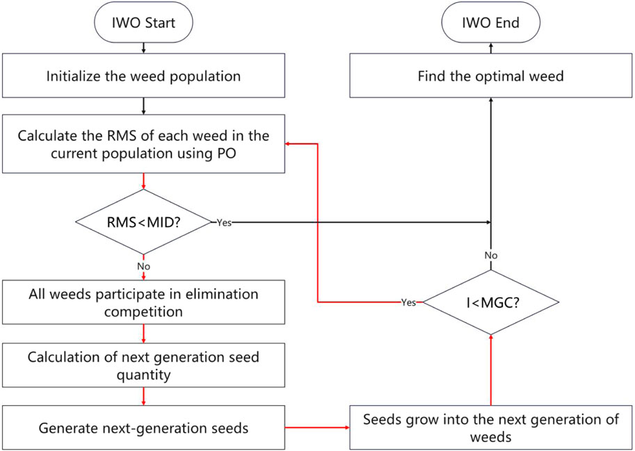
FIGURE 1. Estimation process of hyperparameters.

Step 1. Initialize parameters and weed populations. The starting weed population is randomly generated. The population contains multiple weeds, and each weed consists of two variables, Moho density contrast and average Moho depth. The two variables were randomly generated for individuals within the search interval, and finally the initialization of a single individual was completed. The execution was repeated $MWS$ times to finish the initialization of the population.

Step 2. Calculate the RMS of each current weed. Traversing each individual weed of the population, the two variables of the individual are used as inputs to obtain the corresponding Moho topography based on Equation 1. Based on this, comparing with the corresponding Moho depth of the seismic points, the RMS of the difference between the two is obtained.

Step 3. Traverse the RMS of weed individuals within the current population, if there exists an individual with RMS less than $MID$, it means that the optimal hyperparameter vector is found, go to step 9, and the whole process ends. Otherwise, turn to step 4.

Step 4. All weeds participate in the elimination competition. If the current number of weeds does not exceed $MWS$, then there is no need to participate in the elimination competition. Otherwise, all weeds are sorted according to RMS from smallest to largest, and the top $MWS$ weeds are taken to enter into the next-generation of reproduction, while all other weeds are eliminated. Because the smaller the RMS, the better the weed performs, weeds with larger RMS are eliminated. Turn to step 5.

Step 5. Next-generation seed count calculation. Traverse each weed and calculate the number of seeds $S{N}_i$ by using Eq. 2.

$S{N}_i=MinN+\frac{\left(C{R}_i-MinR\right)}{\left(MaxR-MinR\right)}*\left(MaxN-MinN\right)(2)$

Where $C{R}_i$ denotes the RMS of the current weed, and $MaxR$ and $MinR$ are the maximum and minimum values of the RMS in the current population, respectively. The larger $C{R}_i$ is, the larger $S{N}_i$ is, and vice versa, the less. That is, when the weed population is farther away from the optimal solution, more seeds need to be generated for searching, and when the weed population is closer to the optimal solution, it can be ensured that each weed has at least $MinN$ seeds for searching. Turn to step 6.

Step 6. Generate next-generation seeds. Update $Sigma$ based on the current number of iterations $I$, as shown in Eq. 3. Traverse each weed and execute Eqs 4, 5 to generate $S{N}_i$ seeds for the current weed. Until the traversal is completed, the next-generation seed is obtained. Turn to step 7.

$Sigma=MID+{\left(\frac{MGC-I}{MGC}\right)}^{NLF}*\left(ID-MID\right)(3)$

$C_n=C_i+N\left(0,\frac{Sigma}{30}\right)(4)$

$D_n=D_i+N\left(0,Sigma\right)(5)$

where $C_n$ and $D_n$ are the Moho density contrast and average Moho depth corresponding to the next-generation of seeds, respectively, $C_i$ and $D_i$ are the Moho density contrast and average Moho depth corresponding to the current weed, respectively, and $N\left(x,y\right)$ is a Gaussian distribution with mean $x$ and standard deviation $y$.

Step 7. Seeds grow into next-generation weeds. At this point the next-generation of seeds has grown into a weed and the population is made up of the parent weed and the offspring weed, iteration number $I=I+1$. Go to step 8.

Step 8. If $I>MGC$, go to step 9, the optimal hyperparameter vector is the gene of the weed individual with the smallest RMS in the current population. Otherwise go to step 2.

Step 9. Find the optimal vector. When this step is reached, it indicates the end of the whole IWO process, when the optimal hyperparameter vector has been searched.

3 Synthetic tests

3.1 Airy-isostatic model

To validate the method in this paper, we did synthetic tests in the SCS (110°E∼121°E, 9°N∼22°N). Firstly, an average mantle density ${\rho }_m$ of 3.287 g/cm³ was obtained from the CRUST 1.0 model (Laske et al., 2013), and by subtracting the reference crustal density ${\rho }_c$ (2.67 g/cm³), a Moho density contrast of 0.617 g/cm³ was obtained for the model. In order to reduce the marginal effects generated by the inversion later in the paper, all models in this paper are expanded by 5° in all directions (i.e., ranging from 105°E to 126°E, 4°N to 27°N). Based on the existing ETOPO1 terrain model (Amante and Eakins, 2009), we use Airy-isostatic theory to calculate the Moho topography $m_A$ of the region, as shown in Eq. 1.

$m_A=H-\frac{{\rho }_t}{{\rho }_c-{\rho }_m}h(6)$

Where $H$ is the average compensation depth, taken as 23.4 km (from the average Moho depth of the CRUST 1.0 model). $h$ is the topographic load, taken as the topographic height. ${\rho }_t$ is the topographic density, where ${\rho }_t$ is 2.67 g/cm3 when $h\ge 0$ and ${\rho }_t$ is 1.64 g/cm3 when $h<0$. It can be seen that the Airy Moho topography in the region is shown in Figure 2A, which has an average Moho depth $z_0$ of 20.33 km. 100 Moho depth control points were randomly selected from Figure 2A, as shown in Figure 2B. In addition, based on Figure 2 a) and the available inversion parameters (Moho density contrast of 0.617 g/cm3 and an average Moho depth of 20.33 km), we forward its gravity effect using Parker’s method (Parker, 1973) as shown in Figure 2 c).

FIGURE 2

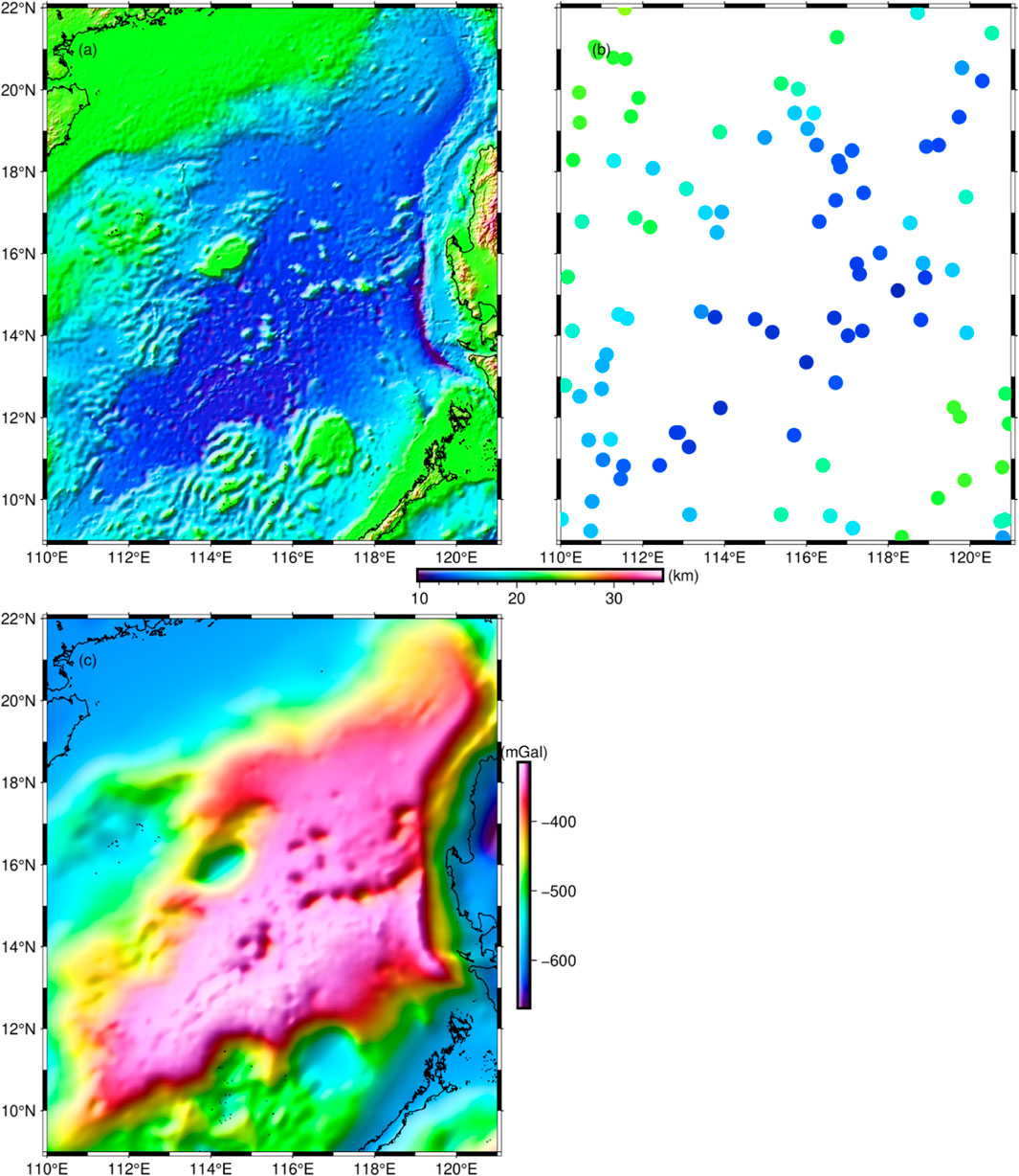
FIGURE 2. Synthetic data in the SCS. (A) Airy-isostasy model. (B) Synthetic seismic control points. (C) Synthetic gravity observations.

3.2 Parameter estimation

In order to compare the differences of different methods in estimating hyperparameters, the improved linear regression method (Li et al., 2022) and IWO are selected in this paper. Based on the synthetic gravity observations (Figure 2C) and the synthetic Moho depth of the control points (Figure 2B), the corresponding hyperparameters are estimated and compared with the true values, respectively, and the results are shown in Table 1.

TABLE 1

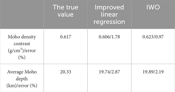
TABLE 1. Accuracy, efficiency statistics of different methods.

At first, the method used was the improved linear regression method. Based on the gravity observations and the Moho depth of the control point, the linear relationship between the two was calculated, as shown in Figure 3A. From its linear intercept (the Moho depth at the control point corresponding to a gravity observation of 0), an average Moho depth of 19.75 km can be obtained, which differs from the true value by 0.58 km. In addition, the corresponding Moho density contrast are estimated by robust linear regression, as shown in Figure 3B. The slope of Figure 3B is the reciprocal of the estimated Moho density contrast, which was calculated to be 0.606 g/cm³, with a difference of 0.011 g/cm³ from the true value. Overall, the Moho density contrast estimated by the method are closer to the true value, but the average Moho depth is still somewhat deviated from the true value.

FIGURE 3

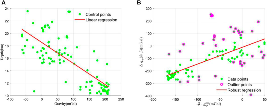
FIGURE 3. Improved linear regression proposed by Li et al. (2022). (A) Estimation of mean Moho topography. (B) Estimation of Moho density contrast.

Next, the method used was IWO. based on IWO, this paper calculated the distribution of weeds for different generations as shown in Figure 4 (the horizontal coordinate is the Moho density contrast, the vertical coordinate is the average Moho depth, and the colours represent the RMS of the difference between the Moho depth and the seismic point depth). Figure 4A shows the first generation of weeds, the distribution of the population is relatively discrete, and the inversion parameters corresponding to each individual weed are significantly different from the actual true values. Figure 4B shows the second generation of weeds, the distribution of populations converges near the true value, and the corresponding average Moho depth is basically in the range of 17–22 km. In this paper, we find the optimal average Moho depth and Moho density contrast in the second generation weed population, which are 19.89 km and 0.623 g/cm³, respectively, with deviations from the true values of 0.46 km and 0.006 g/cm³. Compared with the improved linear regression method, the hyperparameters estimated by IWO are closer to the true values.

FIGURE 4

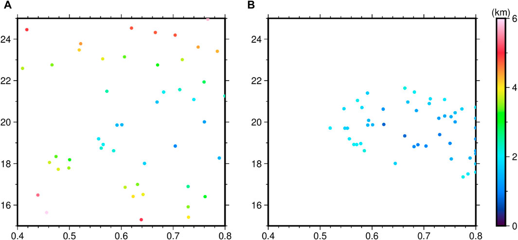
FIGURE 4. Population distributions at different generations. (A) first generation, (B) 2nd generation.

3.3 The influence of noise

Considering that the real gravity observation data and seismic data have noise, which will have a direct impact on the inversion of Moho topography. Therefore, in order to verify the anti-noise ability of IWO, this paper adds Gaussian noise with mean value 0 and standard deviation 2 km to the seismic data of Figure 2B, as shown in Figure 5A. Meanwhile, the gravity observation data of Figure 2C is also added with Gaussian noise with mean value 0 and standard deviation 5 mGal, as shown in Figure 5B. Based on these two noise added data, we use IWO to obtain the weed populations of different generations, as shown in Figure 6. Figure 6 shows the distribution of weed populations from the first to the eighth generation, respectively, and it can be seen that along with several iterations of weed populations, there is an increasing concentration of individual weeds. In the presence of noise, the optimal average Moho depth and Moho density contrast were found to be 19.92 km and 0.614 g/cm³, respectively, from the eighth generation of weed populations. A difference of 0.04 km was found in the average Moho depth and 0.009 g/cm³ in the Moho density contrast, compared to the previous results without noise. In the presence of noise, the deviations of the results in this paper from the true values are 0.41 km and 0.003 g/cm³, which are closer to the true values than the other results in Table 1. It can be seen that the IWO is still valid in the presence of noise.

FIGURE 5

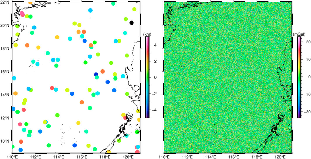
FIGURE 5. Noise in synthetic data.

FIGURE 6

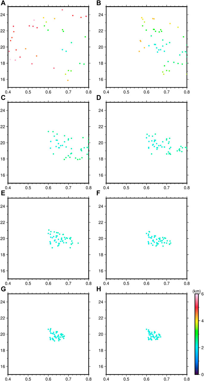
FIGURE 6. Population distributions at different generations under noise. (A) first generation. (B) 2nd generation. (C) third generation. (D) fourth generation. (E) fifth generation. (F) sixth generation. (G) seventh generation. (H) eighth generation.

4 Moho topography in the SCS

4.1 Study area

The study area of this paper ranges from 110°E to 121°E and 9°N to 22°N, with a topographic height of −5,132 m–2,683.9 m, as shown in Figure 7. The region consists of three major sub-basins: the Southwest Sub-Basin (SWSB), the Northwest Sub-Basin (NWSB), and the Eastern Sub-Basin (ESB). In addition, there are the Pearl River Mouth Basin (PRMB), Southeast Hainan Basin (SEHB), Ligue Basin (LYB), Southwest Taiwan Basin (SWTB), Northwest Palawan Basin (NWPB), Zhongjiannan Basin (ZJNB), and Manila Trench (MT), among others. The SCS has experienced a complex evolutionary period in the Cenozoic era, ranging from continental margin rifting, seafloor spreading to subduction collision, leaving abundant traces of seafloor spreading evolution in the marginal seas. Studying the Moho topography in the SCS will help to understand the internal dynamical mechanism of the tectonic evolution in the SCS.

FIGURE 7

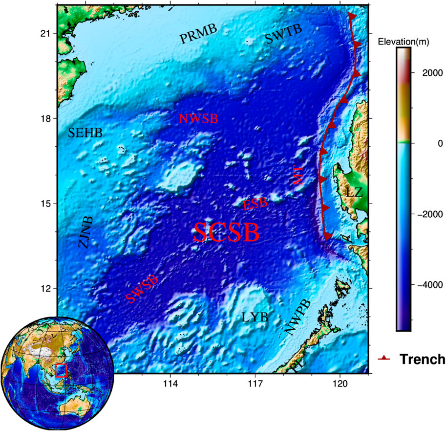
FIGURE 7. Topography of the SCS. The darkred solid line is the Manila Trench (MT); SWSB, Southwest Sub-basin; NWSB, Northwest Sub-basin; ESB, East Sub-basin; LYB, Ligue Basin; ZJNB, Zhongjiannan Basin; PRMB, Pear River Mouth basin; SWTB, Southwest Taiwan basin; SEHB, Southeast Hainan basin; NWPB, Northwest Palawan basin; LZ, Luzon Island.

4.2 Data

There are three main publicly available Datasets used in this paper: 1) The ETOPO1 model (Amante and Eakins, 2009) with a spatial resolution of 1′×1′was used for the topographic data, as shown in Figure 7. 2) Sediment thickness was adopted from the Globsed-v3 model (Straume et al., 2019) with a spatial resolution of 5′× 5′, as shown in Figure 8A. 3) The gravity data used is the XGM 2019e_2159 model (Zingerle et al., 2020) with a spatial resolution of 2′× 2′.

FIGURE 8

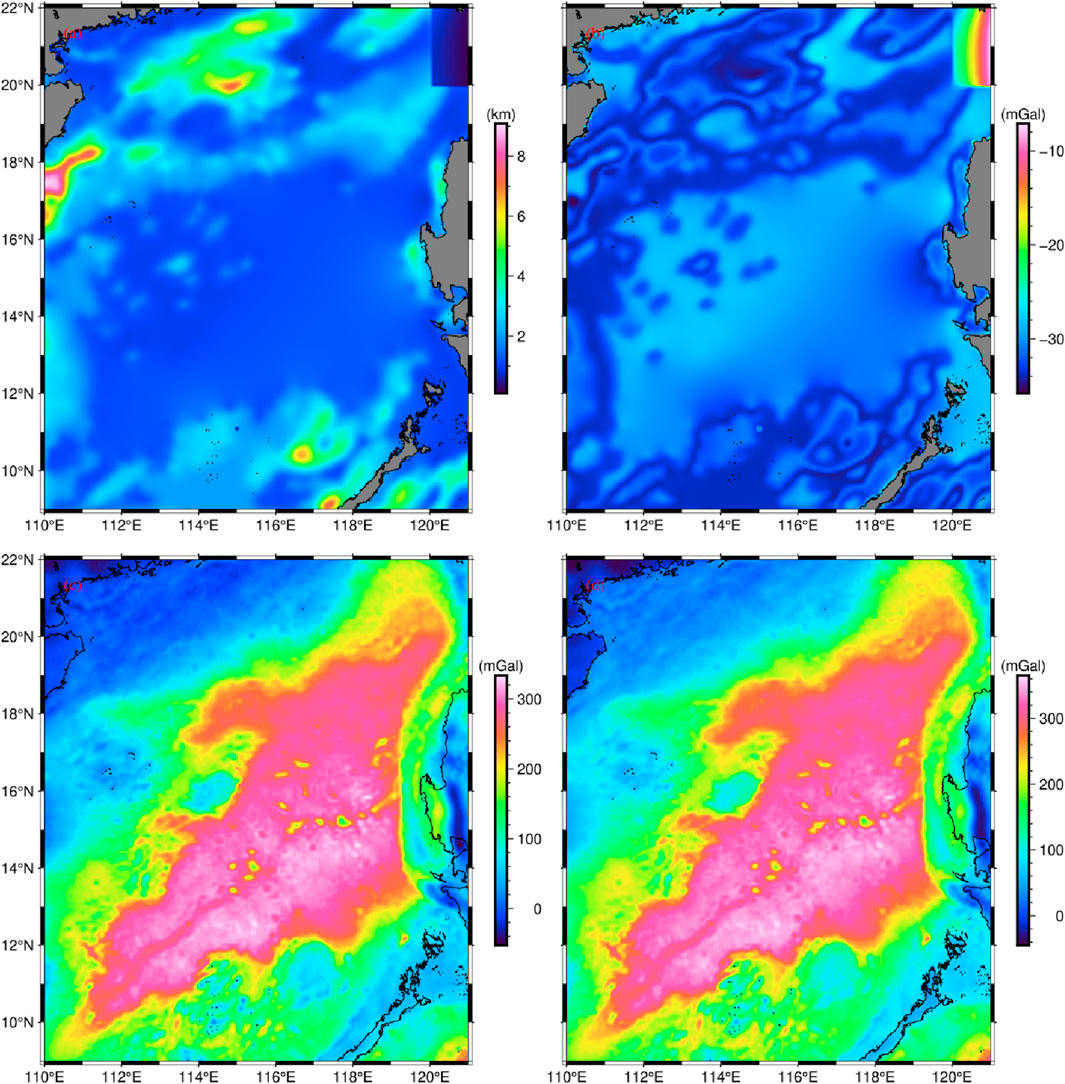
FIGURE 8. Sediment thickness (A) and corresponding gravitational effects (B). (C) Bouguer gravity anomaly. (D) Sediment-free gravity anomalies.

The seismic control point data in this paper are shown in Figure 9, which are mainly from the existing ocean bottom seismometer (OBS) data, including several survey lines such as OBS 2011, OBS973-1, OBS973-2, OBS 2006-2, OBS2013-ZN, OBS2014-ZN, OBS 2017-2, OBS973-3, OBSGS80 (Nissen et al., 1995; Pin et al., 2001; Qiu et al., 2001; Huang et al., 2005; Wang et al., 2006; Luo et al., 2009; Qiu et al., 2011; Wei et al., 2011; Ao et al., 2012; McIntosh et al., 2014; Pichot et al., 2014; Ruan et al., 2016; Zhang et al., 2016; Wu et al., 2017; Yu et al., 2017; Zhao et al., 2018; Huang et al., 2019; Li et al., 2020; Wang et al., 2020; Zhang et al., 2020; Li et al., 2021). In addition, some of the seismic control point data were derived from sonar data (Qin et al., 2011). In order to make effective use of the seismic data, this paper divided the seismic data into test points (circles in Figure 9) and validation points (triangles in Figure 9). Among them, the test points are used to estimate the average Moho depth and Moho density contrast in the SCS, and the validation points are used to evaluate the accuracy of the Moho topographic model.

FIGURE 9

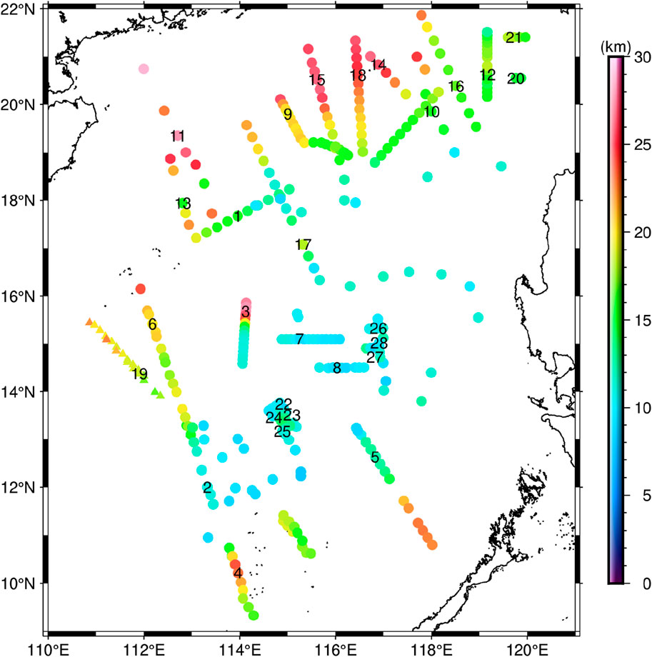
FIGURE 9. Seismic control points in the SCS.

Circles are test points for the estimation of hyperparameters. Triangles are validation points for estimating the accuracy of the Moho topography. Different numbers in the figure represent different seismic lines. Among them, line 1 is OBS 2006-2 (Ao et al., 2012), line 2 is OBS 2011-1 (Yu et al., 2017; Huang et al., 2019), line 3 is OBS 2017-2 (Li et al., 2020; 2021), line 4 is OBS973-1 (Qiu et al., 2011), line 5 is OBS973-2 (Qiu et al., 2011), line 6 is OBS973-3 (Qiu et al., 2011), line 7 is OBS2013-ZN (Ruan et al., 2016), line 8 is OBS2014-ZN (Ruan et al., 2016), line 9 is DSRP 2002 (Huang et al., 2005), line 10 is ESP1985-E (Nissen et al., 1995), line 11 is ESP1985-W (Nissen et al., 1995), line 12 is MGL0908-3 (McIntosh et al., 2014), line 13 is OBH 1996-4 (Qiu et al., 2001), line 14 is OBS863 (Luo et al., 2009; Wu et al., 2017), line 15 is OBS 1993 (Pin et al., 2001), line 16 is OBS 2001 (Wang et al., 2006), line 17 is OBS 2006-1 (Wu et al., 2012), line 18 is OBS 2006-3 (Wei et al., 2011), line 19 is OBS 2011 (Pichot et al., 2014; Wu et al., 2017), line 20 is T1 from Wu et al. (2017), line 21 is T2 from Wu et al. (2017), line 22 is T1 from Zhang et al. (2016) and Zhang et al. (2020), line 23 is T2 from Zhang et al. (2020), line 24 is T3 from Zhang et al. (2020), line 25 is T4 from Zhang et al. (2020), line 26 is P1 from Zhao et al. (2018), line 27 is P3 from Zhao et al. (2018), and line 28 is P4 from Zhao et al. (2018).

We calculated the Bouguer gravity anomaly in the study area based on the free-air gravity anomaly corresponding to the XGM 2019e_2159 model and the ETOPO1 model, as shown in Figure 8C. Due to the consideration of the effect brought by the sedimentary layer, based on the Globsed-v3 model, this paper calculated the gravity effect corresponding to the sedimentary layer by using Parker’s method (Parker, 1973), as shown in Figure 8B. By subtracting the gravity effect corresponding to the sedimentary layer from the Bouguer gravity anomaly, we obtained the sediment-free gravity anomaly, as shown in Figure 8D.

In Figure 8D, the gravity anomalies in the study area range from −44.2 mGal to 361.2 mGal. Among them, the gravity anomalies of the SCSB as a whole are on the high side. Most of the SWSB and ESB are higher than 310 mGal, and the gravity anomalies of the NWSB are around 300 mGal. The upper left corner in the study area contains ZJMB, SWTB, SEHB, and ZJNB, and the area is dominated by continental shelf with relatively low gravity anomalies, most of the area is below 100 mGal. In addition, the gravity anomalies of LYB and NWPB are around 100 mGal.

4.3 Moho topographic inversion

In order to invert a finer Moho topography in the SCS, the first step that needs to be determined is the inversion parameters (Moho density contrast and average Moho depth) for the region. Here, the sediment-free gravity anomaly is assumed to be associated only with the undulation of the Moho surface, and based on this gravity anomaly and the seismic test points (circles in Figure 9), we calculated the distribution of weeds for different generations using IWO, as shown in Figure 10.

FIGURE 10

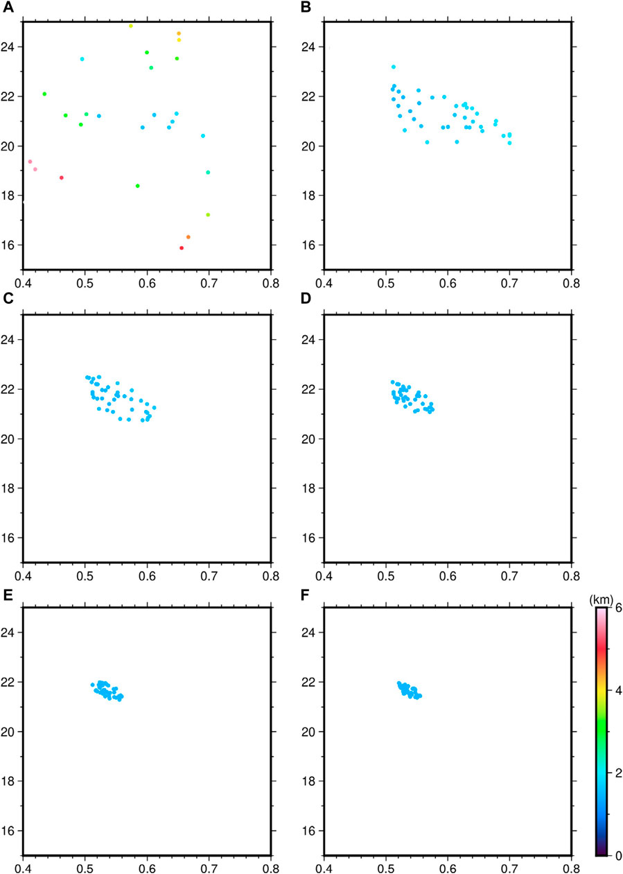
FIGURE 10. Population distributions at different generations. (A) first generation. (B) third generation. (C) fifth generation. (D) seventh generation. (E) ninth generation. (F) 12th generation.

In Figure 10, we showed the population distribution of the first a), third b), fifth c), seventh d), ninth e) and 12th f) generations, respectively. It can be seen that the population distribution of the first generation is more discrete, covering almost the entire search space. The population distributions of the third, fifth and seventh generations begin to cluster slowly, suggesting that the likelihood interval of the inversion parameters is decreasing. When iterating to the ninth and 12th generations, the RMS corresponding to the weed individuals is almost around 1.0 km, reaching a stable state. In this case, the optimal weed individual is selected from the population, which corresponds to the optimal parameters of Moho topographic inversion.

Under the constraints of seismic control points, this paper finds the optimal weed individual, whose corresponding Moho density contrast and average Moho depth are 0.535 g/cm³ and 21.63 km, respectively. Based on these two parameters, the Moho topography of the SCS is obtained by using Eq. 1, as shown in Figure 11.

FIGURE 11

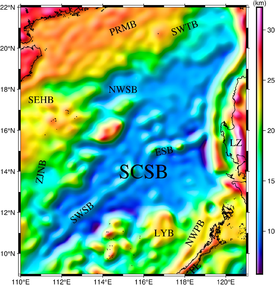
FIGURE 11. Moho topography in the SCS.

Figure 11 shows that the Moho surface in the study area is distinctly undulating, ranging between 5.7 km and 32.3 km overall. Among them, the shallowest part of the Moho surface is close to 6 km, and there are two main areas, the first one is located in the southern part of SWSB, roughly ranging from 113.3°E to 114°E, 10.8°N to 11.5°N. The second one is located in the southern part of MT, roughly ranging from 118.8°E to 119.1°E, 13.9°N to 15.5°N. The deepest part of the Moho surface in the study area is mainly concentrated in the LZ, which roughly ranges from 120.5°E to 121°E and 14°N to 16°N, and its Moho surface is around 31 km. Compared to other regions, the SCSB has significant mantle uplift, with an overall Moho surface of less than 15 km. of which, with the exception of some seamounts, is essentially around 13 km in the ESB and NWSB. It is worth mentioning that there is a clear asymmetry in the Moho surface on the north and south sides of the SWSB, bounded by the spreading ridge. The Moho surface on the south side of the spreading ridge is shallower, with depths ranging from 6 to 10 km. On the other hand, the Moho surface on the northern side is deeper, with depths generally ranging from 10 to 13 km. The Moho surface in the continental shelf area, such as ZJMB, SEHB, NWPB, etc., is basically between 21 and 26 km. In addition, the Moho surface of LYB is around 23 km.

Previously, the CRUST 1.0 model was the internationally known Moho topography model (Laske et al., 2013), as shown in Figure 12 a). In this paper, a new Moho topographic model (Model A) is computed using the improved Bott’s method (Li et al., 2022), as shown in Figure 12 b). To verify the accuracy of the Moho topographic model in this paper, the seismic validation points (triangles in Figure 9) and all seismic points were used as a control group, and Table 2 demonstrated the differences between the CRUST 1.0 model, Model A, and the model in this paper. As can be seen, in comparison with the all seismic points, the RMS of the CRUST 1.0 model is 4.4 km, the RMS of model A is 1.9 km, and the RMS of the model in this paper is 1.4 km. In addition, in the comparison with the seismic validation points, the RMS of CRUST 1.0 model is 3.9 km, the RMS of Model A is 2.5 km, and the RMS of the model in this paper is 1.3 km. Compared with the CRUST 1.0 model and Model A, the RMS of the model in this paper has a significant reduction, which is closer to the real situation. Moreover, this also verified the reliability of IWO in Moho topographic inversion.

FIGURE 12

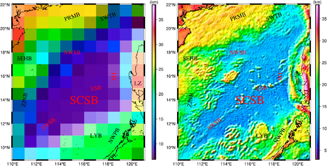
FIGURE 12. Moho topography from the CRUST 1.0 model (A) and the Model A (B).

TABLE 2

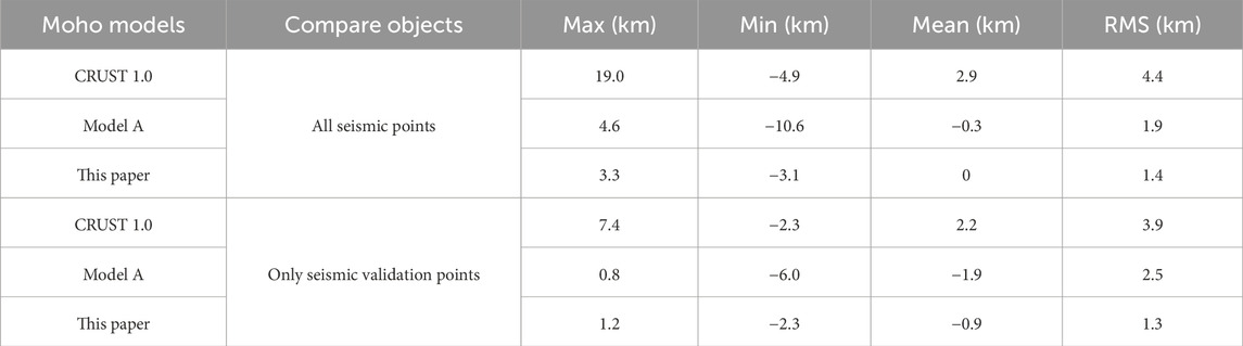
TABLE 2. Comparison of different Moho topography models and seismic Moho depth.

5 Conclusion

Based on the advantages of IWO in solving nonlinear problems, this paper proposed to improve the existing Parker-Oldenburg method with IWO. Under the constraint of seismic control points, more accurate Moho density contrast and average Moho depth are estimated, which in turn invert the fine Moho topography of SWSB. In the synthetic tests, the errors of Moho density contrast and average Moho depth estimated by IWO were 0.97% and 2.19%, respectively, each of which decreased compared to the improved linear regression method, indicating that the parameters estimated by this method are closer to the true values. This suggests that IWO has a clear advantage in estimating Moho density contrast and mean Moho depth, and this in turn provides a basis for estimating a more accurate Moho topography. In practical application, based on the XGM 2019e_2159 gravity field model and the seismic control point data, this paper estimated the Moho density contrast and the average Moho depth of the SCS to be 0.623 g/cm³ and 19.89 km, respectively, by using IWO, and then inverted Moho topography of the SCS. The Moho topography shows that the Moho surface in the study area ranges from 5.7 to 32.3 km, among which, the Moho surface in the South China Sea Basin is less than 15 km, with obvious mantle uplift phenomenon. By comparing with the seismic validation points, the RMS of the difference between it and the Moho topographic model in this paper is 1.3 km, which is more consistent with the actual situation compared with other Moho surface models. This depends on more precise Moho density contrast and average Moho depth, which also fully confirms that IWO is effective.

6 Discussion

In order to show the difference between the Moho topographic model in this paper (Figure 11) and the seismic data (Figure 9), we extracted the Moho depths at the seismic points of the two and made the difference, and the results are shown in Figure 13. Figure 13A shows that the depth difference at seismic points in the study area ranges from −3 to 3 km, and most of the survey lines have depth differences within plus or minus 1 km (appearing as light green or light blue), which suggests that the Moho topographic model in this paper performs better and is close to the seismic data. Among them, the depth difference at seismic points in SCSB is small, ranging from −2 km to 2 km. Some seismic lines in the northern (e.g., PRMB) and southern (e.g., LYB) parts of the South China Sea have large differences from the Moho topographic model in this paper, with some seismic points having differences of about 3 km. In order to find the relationship between depth differences and sediments, we extracted the corresponding sediment thicknesses based on the distribution of points in Figure 13A, as shown in Figure 13B. In Figures 13A,A few lines have large depth differences. Combined with Figure 13B, it can be seen that these survey lines are mainly located in areas with thick sedimentary layers, and it is possible that the sedimentary layers are affecting the seismic results. Based on previous research (Holbrook et al., 1996; Loureiro et al., 2016; Wang et al., 2020), we consider that this effect stems from two sources. One is that complex sedimentary basins pose modelling challenges, which may lead to biases in interface depths due to systematic under or over estimations of propagation velocities. The second is that different OBS spacing changes the sensitivity of the detection technique to the sedimentary layers. If they are too far apart, it is not possible to extract propagation velocities from the topmost layers. Any lateral variation in propagation velocity in the sediment will propagate as uncertainty in the lower structures. Of course, this bias does not have a large impact on the estimation of the inversion parameters in this paper because multiple survey lines are used and most of them correspond to more accurate results.

FIGURE 13

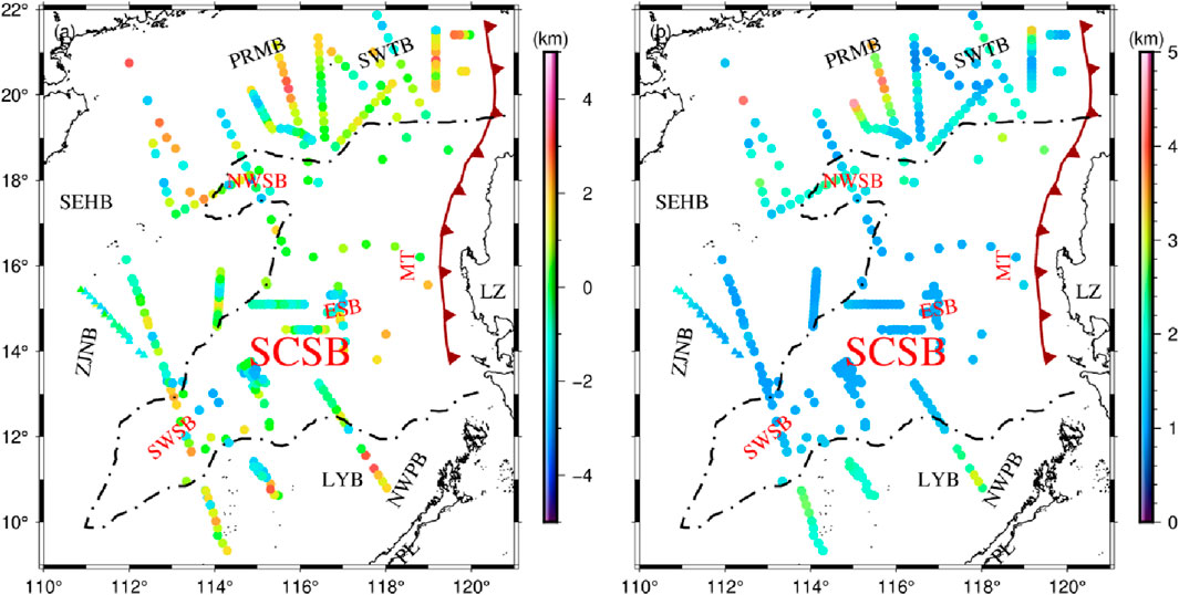
FIGURE 13. (A) Difference between Moho topographic model and seismic data. (B) Sediment thickness corresponding to seismic points.

Data availability statement

The original contributions presented in the study are included in the article/Supplementary Material, further inquiries can be directed to the corresponding authors.

Author contributions

HZ: Writing–original draft. HY: Writing–original draft, Writing–review and editing. CX: Writing–original draft, Writing–review and editing. RL: Writing–review and editing. LB: Writing–review and editing. QH: Writing–review and editing. YL: Writing–review and editing. JL: Writing–review and editing. YX: Writing–review and editing. YL: Writing–review and editing.

Funding

The author(s) declare financial support was received for the research, authorship, and/or publication of this article. This work was supported by the NSFC-Guang-dong Joint Fund (Grant Nos. U20A20100), the National Natural Science Foundation of China (42104136, 41974014, 42274004), the China Geological Survey (DD20230649, DD20191007, DD20221714), and the Natural Science Foundation of Guangdong Province (2022A1515010396), with thanks to the Western Australian Geodesy Group, Zingerle et al. (2020), Amante and Eakins (2009), Straume et al. (2019) and Laske et al. (2013) for data support. Dedicated Fund for Marine Economic Development in Guangdong Province (GDNRC[2023]40).

Conflict of interest

The authors declare that the research was conducted in the absence of any commercial or financial relationships that could be construed as a potential conflict of interest.

Publisher’s note

All claims expressed in this article are solely those of the authors and do not necessarily represent those of their affiliated organizations, or those of the publisher, the editors and the reviewers. Any product that may be evaluated in this article, or claim that may be made by its manufacturer, is not guaranteed or endorsed by the publisher.

References

Amante, C., and Eakins, B. (2009). ETOPO1 1 arc-minute global relief model:procedures, data sources and analysis. Natl. Geophys. Data Cent. 10 (2009), V5C8276M. doi:10.7289/V5C8276M

CrossRef Full Text | Google Scholar

Ao, W., Zhao, M. H., Qiu, X. L., Ruan, A. G., and Li, J. B. (2012). Crustal structure of the northwest sub-basin of the South China Sea and its tectonic implication. Earth Science-Journal China Univ. Geosciences 37 (4), 779–790.

Google Scholar

Dong, M., Wu, S., Zhang, J., Xu, X., Gao, J., and Song, T. (2020). Lithospheric structure of the Southwest south China sea:implications for rifting and extension. Int. Geol. Rev. 62 (7-8), 924–937. doi:10.1080/00206814.2018.1539926

CrossRef Full Text | Google Scholar

Eldosouky, A. M., Pham, L. T., El-Qassas, R. A. Y., Hamimi, Z., and Oksum, E. (2021). Lithospheric structure of the Arabian–Nubian shield using satellite potential field data. Geol. Arabian-Nubian shield, 139–151. doi:10.1007/978-3-030-72995-0_6

CrossRef Full Text | Google Scholar

Floberghagen, R., Fehringer, M., Lamarre, D., Muzi, D., Frommknecht, B., Steiger, C., et al. (2011). Erratum to:Mission design, operation and exploitation of the Gravity field and steady-state Ocean Circulation Explorer (GOCE) mission. J. Geodesy 85, 749–758. doi:10.1007/s00190-011-0498-3

CrossRef Full Text | Google Scholar

Florio, G. (2020). The estimation of depth to basement under sedimentary basins from gravity data:Review of approaches and the ITRESC method, with an application to the Yucca Flat Basin (Nevada). Surv. Geophys. 41 (5), 935–961. doi:10.1007/s10712-020-09601-9

CrossRef Full Text | Google Scholar

Florio, G., Milano, M., and Cella, F. (2021). Gravity mapping of basement depth in seismogenic, fault-controlled basins:The case of Middle Aterno Valley (Central Italy). Tectonophysics 817, 229044. doi:10.1016/j.tecto.2021.229044

CrossRef Full Text | Google Scholar

Gozzard, S., Kusznir, N., Franke, D., Cullen, A., Reemst, P., and Henstra, G. (2019). South China Sea crustal thickness and oceanic lithosphere distribution from satellite gravity inversion. Pet. Geosci. 25 (1), 112–128. doi:10.1144/petgeo2016-162

CrossRef Full Text | Google Scholar

Holbrook, W. S., Brocher, T. M., ten Brink, U. S., and Hole, J. A. (1996). Crustal structure of a transform plate boundary: San Francisco Bay and the central California continental margin. J. Geophys. Res. Solid Earth 101 (B10), 22311–22334. doi:10.1029/96JB01642

CrossRef Full Text | Google Scholar

Huang, C., Zhou, D., Sun, Z., Chen, C., and Hao, H. (2005). Deep crustal structure of Baiyun Sag, northern South China Sea revealed from deep seismic reflection profile. Chin. Sci. Bull. 50, 1131–1138. doi:10.1360/04wd0207

CrossRef Full Text | Google Scholar

Huang, H., Qiu, X., Pichot, T., Klingelhoefer, F., Zhao, M., Wang, P., et al. (2019). Seismic structure of the northwestern margin of the South China Sea:implication for asymmetric continental extension. Geophys. J. Int. 218 (2), 1246–1261. doi:10.1093/gji/ggz219

CrossRef Full Text | Google Scholar

Huang, L., Wen, Y., Li, C. F., Peng, X., Lu, Z., Xu, L., et al. (2023). A refined Moho depth model from a joint analysis of gravity and seismic data of the South China Sea basin and its tectonic implications. Phys. Earth Planet. Interiors 334, 106966. doi:10.1016/j.pepi.2022.106966

CrossRef Full Text | Google Scholar

Kornfeld, R. P., Arnold, B. W., Gross, M. A., Dahya, N. T., Klipstein, W. M., Gath, P. F., et al. (2019). GRACE-FO:The gravity recovery and climate experiment follow-on mission. J. Spacecr. Rockets 56 (3), 931–951. doi:10.2514/1.A34326

CrossRef Full Text | Google Scholar

Laske, G., Masters, G., Ma, Z., and Pasyanos, M. (2013). “Update on CRUST1.0 – a 1-degree global model of Earth’s crust,”in EGU general assembly conference abstracts.

Google Scholar

Lei, J. P., Jiang, S. H., Li, S. Z., Gao, S., Zhang, H. X., Wang, G., et al. (2016). Gravity anomaly in the southern South China Sea:a connection of Moho depth to the nature of the sedimentary basins' crust. Geol. J. 51, 244–262. doi:10.1002/gj.2817

CrossRef Full Text | Google Scholar

Li, C. F., and Wang, J. (2016). Variations in Moho and curie depths and heat flow in eastern and southeastern asia. Mar. Geophys. Res. 37, 1–20. doi:10.1007/s11001-016-9265-4

CrossRef Full Text | Google Scholar

Li, J., Xu, C., and Chen, H. (2022). An improved method to Moho depth recovery from gravity disturbance and its application in the South China Sea. J. Geophys. Research:Solid Earth 127 (7). doi:10.1029/2022JB024536

CrossRef Full Text | Google Scholar

Li, Y., Huang, H., Grevemeyer, I., Qiu, X., Zhang, H., and Wang, Q. (2021). Crustal structure beneath the Zhongsha Block and the adjacent abyssal basins, South China Sea:New insights into rifting and initiation of seafloor spreading. Gondwana Res. 99, 53–76. doi:10.1016/j.gr.2021.06.015

CrossRef Full Text | Google Scholar

Li, Y., Huang, H., Qiu, X., Dang, Y., Sun, X., Zhang, L., et al. (2020). OSmfs: an online interactive tool to evaluate prognostic markers for myxofibrosarcoma. Chin. J. Geophys. 63 (4), 1523–1537. doi:10.3390/genes11121523

CrossRef Full Text | Google Scholar

Loureiro, A., Afilhado, A., Matias, L., Moulin, M., and Aslanian, D. (2016). Monte Carlo approach to assess the uncertainty of wide-angle layered models: application to the Santos Basin, Brazil. Tectonophysics, 683: 286–307. doi:10.1016/j.tecto.2016.05.040

CrossRef Full Text | Google Scholar

Luo, W. Z., Yan, P., Wen, N., and Wang, L. (2009). Ocean-Bottom seismometer experiment over chaoshan sag in the northern south China Sea. J. Trop. Oceanogr. 28 (4), 59–65.

Google Scholar

McIntosh, K., Lavier, L., van Avendonk, H., Lester, R., Eakin, D., and Liu, C. S. (2014). Crustal structure and inferred rifting processes in the northeast South China Sea. Mar. Petroleum Geol. 58, 612–626. doi:10.1016/j.marpetgeo.2014.03.012

CrossRef Full Text | Google Scholar

Mehrabian, A. R., and Lucas, C. (2006). A novel numerical optimization algorithm inspired from weed colonization. Ecol. Inf. 1 (4), 355–366. doi:10.1016/j.ecoinf.2006.07.003

CrossRef Full Text | Google Scholar

Melouah, O., Ebong, E. D., Abdelrahman, K., and Eldosouky, A. M. (2023). Lithospheric structural dynamics and geothermal modeling of the Western Arabian Shield. Sci. Rep. 13 (1), 11764. doi:10.1038/s41598-023-38321-4

PubMed Abstract | CrossRef Full Text | Google Scholar

Melouah, O., Eldosouky, A. M., and Ebong, E. D. (2021). Crustal architecture, heat transfer modes and geothermal energy potentials of the Algerian Triassic provinces. Geothermics 96, 102211. doi:10.1016/j.geothermics.2021.102211

PubMed Abstract | CrossRef Full Text | Google Scholar

Nissen, S. S., Hayes, D. E., Bochu, Y., Zeng, W., Chen, Y., and Nu, X. (1995). Gravity, heat flow, and seismic constraints on the processes of crustal extension: northern margin of the South China Sea. J. Geophys. Res. solid earth 100 (B11), 22447–22483. doi:10.1029/95JB01868

CrossRef Full Text | Google Scholar

Niu, X. W., Wei, X. D., Ruan, A. G., and Wu, Z. (2014). Comparision of inversion method of wide angle Ocean Bottom Seismometer profile: a case study of profile OBS973-2 across Ligue bank in the South China Sea. Chin. J. Geophys. 57 (8), 2701–2712. doi:10.6038/cjg20140828

CrossRef Full Text | Google Scholar

Oldenburg, D. W. (1974). The inversion and interpretation of gravity anomalies. Geophysics 39 (4), 526–536. doi:10.1190/1.1440444

CrossRef Full Text | Google Scholar

Parker, R. L. (1973). The rapid calculation of potential anomalies. Geophys. J. Int. 31 (4), 447–455. doi:10.1111/j.1365-246X.1973.tb06513.x

CrossRef Full Text | Google Scholar

Pham, L. T., Oksum, E., Eldosouky, A. M., Gomez-Ortiz, D., Abdelrahman, K., Altinoğlu, F. F., et al. (2022). Determining the Moho interface using a modified algorithm based on the combination of the spatial and frequency domain techniques: a case study from the Arabian Shield. Geocarto Int. 37 (25), 10581–10596. doi:10.1080/10106049.2022.2037733

CrossRef Full Text | Google Scholar

Piao, Q., Zhang, B., Zhang, R., Geng, M., and Zhong, G. (2022). Continent-ocean transition in the northern South China Sea by high-quality deep reflection seismic data. Chin. J. Geophys. (in Chinese) 65 (7), 2546–2559. doi:10.6038/cjg2022P0663

CrossRef Full Text | Google Scholar

Pichot, T., Delescluse, M., Chamot-Rooke, N., Pubellier, M., Qiu, Y., Meresse, F., et al. (2014). Deep crustal structure of the conjugate margins of the SW South China Sea from wide-angle refraction seismic data. Marine and Petroleum Geology 58, 627–643. doi:10.1016/j.marpetgeo.2013.10.008

CrossRef Full Text | Google Scholar

Pin, Y., Di, Z., and Zhaoshu, L. (2001). A crustal structure profile across the northern continental margin of the South China Sea. Tectonophysics 338 (1), 1–21. doi:10.1016/S0040-1951(01)00062-2

CrossRef Full Text | Google Scholar

Qin, J., Hao, T., Xu, Y., Huang, S., Lv, C., and Hu, W. (2011). The distribution characteristics and the relationship between the tectonic units of the Moho depth in South China Sea and adjacent areas. Chinese Journal of Geophysics 54 (12), 3171–3183.

Google Scholar

Qiu, X., Ye, S., Wu, S., Shi, X., Zhou, D., Xia, K., et al. (2001). Crustal structure across the xisha trough, northwestern south China Sea. Tectonophysics 341 (1-4), 179–193. doi:10.1016/S0040-1951(01)00222-0

CrossRef Full Text | Google Scholar

Qiu, X. L., Zhao, M. H., Ao, W., et al. (2011). OBS survey and crustal structure of the SW sub-Basin and nansha block, south China Sea. Chinese Journal of Geophysics 54 (6), 1009–1021. doi:10.1002/cjg2.1680

CrossRef Full Text | Google Scholar

Rao, W., Yu, N., Chen, G., Xu, X., Zhao, S., Song, Z., et al. (2023). Moho inversion by gravity anomalies in the South China Sea: updates and improved iteration of the parker-oldenburg algorithm. Earth and Space Science 10 (9). doi:10.1029/2022EA002794

CrossRef Full Text | Google Scholar

Ruan, A., Wei, X., Niu, X., Zhang, J., Dong, C., Wu, Z., et al. (2016). Crustal structure and fracture zone in the Central Basin of the South China Sea from wide angle seismic experiments using OBS. Tectonophysics 688, 1–10. doi:10.1016/j.tecto.2016.09.022

CrossRef Full Text | Google Scholar

Sandwell, D. T., Müller, R. D., Smith, W. H. F., Garcia, E., and Francis, R. (2014). New global marine gravity model from CryoSat-2 and Jason-1 reveals buried tectonic structure. Science 346 (6205), 65–67. doi:10.1126/science.1258213

PubMed Abstract | CrossRef Full Text | Google Scholar

Straume, E. O., Gaina, C., Medvedev, S., Hochmuth, K., Gohl, K., Whittaker, J. M., et al. (2019). GlobSed: updated total sediment thickness in the world's oceans. Geochemistry, Geophysics, Geosystems 20 (4), 1756–1772. doi:10.1029/2018GC008115

CrossRef Full Text | Google Scholar

Tapley, B. D., Bettadpur, S., Watkins, M., and Reigber, C. (2004). The gravity recovery and climate experiment: mission overview and early results. Geophysical Research Letters 31 (9). doi:10.1029/2004gl019920

CrossRef Full Text | Google Scholar

Wan, X., Li, C. F., Zhao, M., He, E., Liu, S., Qiu, X., et al. (2020). Seismic velocity structure of the magnetic quiet zone and continent-ocean boundary in the northeastern South China Sea. Journal of Geophysical Research Solid Earth 124 (11), 11866–11899. doi:10.1029/2019jb017785

CrossRef Full Text | Google Scholar

Wang, Q., Zhao, M., Zhang, H., Zhang, J., He, E., Yuan, Y., et al. (2020). Crustal velocity structure of the Northwest Sub-basin of the South China Sea based on seismic data reprocessing. Science China Earth Sciences 63, 1791–1806. doi:10.1007/s11430-020-9654-4

CrossRef Full Text | Google Scholar

Wang, T. K., Chen, M. K., Lee, C. S., and Xia, K. (2006). Seismic imaging of the transitional crust across the northeastern margin of the South China Sea. Tectonophysics 412 (3-4), 237–254. doi:10.1016/j.tecto.2005.10.039

CrossRef Full Text | Google Scholar

Wei, X., Ruan, A., Zhao, M., Qiu, X., Li, J., Zhu, J., et al. (2011). A wide-angle OBS profile across dongsha uplift and chaoshan depression in the mid-northern south China Sea. Chinese Journal of Geophysics (in Chinese) 54 (12), 3325–3335. doi:10.3969/j.issn.0001-5733.2011.12.030

CrossRef Full Text | Google Scholar

Wu, Z., Gao, J., Ding, W., Shen, Z., Zhang, T., and Yang, C. (2017). Moho depth of the South China Sea basin from three-dimensional gravity inversion with constraint points. Chinese Journal of Geophysics 60 (7), 2599–2613. doi:10.6038/cjg20170709

CrossRef Full Text | Google Scholar

Wu, Z. L., Li, J. B., Ruan, A. G., Lou, H., Ding, W., Niu, X., et al. (2012). Crustal structure of the northwestern sub-basin, South China Sea: results from a wide-angle seismic experiment. Science China Earth Sciences 55, 159–172. doi:10.1007/s11430-011-4324-9

CrossRef Full Text | Google Scholar

Xu, C., Liu, Z., Luo, Z., Wu, Y., and Wang, H. (2017). Moho topography of the Tibetan Plateau using multi-scale gravity analysis and its tectonic implications. Journal of Asian Earth Sciences 138, 378–386. doi:10.1016/j.jseaes.2017.02.028

CrossRef Full Text | Google Scholar

Xuan, S., Jin, S., and Chen, Y. (2020). Determination of the isostatic and gravity Moho in the east China Sea and its implications. Journal of Asian Earth Sciences 187, 104098. doi:10.1016/j.jseaes.2019.104098

CrossRef Full Text | Google Scholar

Yang, J., Liu, C., Chen, T., and Zhang, Y. (2019). The invasive weed optimization–based inversion of parameters in probability integral model. Arabian journal of geosciences 12, 424–429. doi:10.1007/s12517-019-4592-9

CrossRef Full Text | Google Scholar

Yu, Z., Li, J., Ding, W., Zhang, J., Ruan, A., and Niu, X. (2017). Crustal structure of the Southwest Subbasin, South China Sea, from wide-angle seismic tomography and seismic reflection imaging. Marine Geophysical Research 38, 85–104. doi:10.1007/s11001-016-9284-1

CrossRef Full Text | Google Scholar

Zhang, J., Li, J., Ruan, A., Ding, W., Niu, X., Wang, W., et al. (2020). Seismic structure of a postspreading seamount emplaced on the fossil spreading center in the Southwest Subbasin of the South China Sea. Journal of Geophysical ResearchSolid Earth 125 (10). doi:10.1029/2020JB019827

CrossRef Full Text | Google Scholar

Zhang, J., Li, J., Ruan, A., Wu, Z., Yu, Z., Niu, X., et al. (2016). The velocity structure of a fossil spreading centre in the Southwest Sub-basin, South China Sea. Geological Journal 51, 548–561. doi:10.1002/gj.2778

CrossRef Full Text | Google Scholar

Zhao, G., Liu, J., Chen, B., Kaban, M., and Zheng, X. (2020). Moho beneath Tibet based on a joint analysis of gravity and seismic data. Geochemistry, Geophysics, Geosystems 21 (2). doi:10.1029/2019GC008849

CrossRef Full Text | Google Scholar

Zhao, M., He, E., Sibuet, J. C., Sun, L., Qiu, X., Tan, P., et al. (2018). Postseafloor spreading volcanism in the central east South China Sea and its formation through an extremely thin oceanic crust. Geochemistry, Geophysics, Geosystems 19 (3), 621–641. doi:10.1002/2017GC007034

CrossRef Full Text | Google Scholar

Zingerle, P., Pail, R., Gruber, T., and Oikonomidou, X. (2020). The combined global gravity field model XGM2019e. Journal of Geodesy 94 (7), 66. doi:10.1007/s00190-020-01398-0

CrossRef Full Text | Google Scholar