Prediction of permeability in a tight sandstone reservoir using a gated network stacking model driven by data and physical models

Introduction: Permeability is one of the most important parameters for reservoir evaluation. It is commonly measured in laboratories using underground core samples. However, it cannot describe the entire reservoir because of the limited number of cores. Therefore, petrophysicists use well logs to establish empirical equations to estimate permeability. This method has been widely used in conventional sandstone reservoirs, but it is not applicable to tight sandstone reservoirs with low porosity, extremely low permeability, and complex pore structures.

Methods: Machine learning models can identify potential relationships between input features and sample labels, making them a good choice for establishing permeability prediction models. A stacking model is an ensemble learning method that aims to train a meta-learner to learn an optimal combination of expert models. However, the meta-learner does not evaluate or control the experts, making it difficult to interpret the contribution of each model. In this study, we design a gate network stacking (GNS) model, which is an algorithm that combines data and model-driven methods. First, an input log combination is selected for each expert model to ensure the best performance of the expert model and selfoptimization of the hyperparameters. Petrophysical constraints are then added to the inputs of the expert model and meta-learner, and weights are dynamically assigned to the output of the expert model. Finally, the overall performance of the model is evaluated iteratively to enhance its interpretability and robustness.

Results and discussion: The GNS model is then used to predict the permeability of a tight sandstone reservoir in the Jurassic Ahe Formation in the Tarim Basin. The case study shows that the permeability predicted by the GNS model is more accurate than that of other ensemble models. This study provides a new approach for predicting the parameters of tight sandstone reservoirs.

1 Introduction

The absolute permeability, k, is a measure of the ability of a porous medium to pass through a certain fluid in the presence of one or more fluid phases. The accurate prediction of permeability plays an important role in the evaluation of reservoir quality, numerical simulations of reservoirs, and estimation of geological reserves. Rock permeability is usually obtained through laboratory core measurements (Wu, 2004). However, this method is time-consuming and costly, and it has problems such as non-random sampling locations and limited quantity, making it impossible to characterize the permeability characteristics of the entire reservoir.

Scholars have performed extensive research on the problem of permeability predictions. The Kozeny-Carman equation (KC equation) based on the tube-like model applies the porosity and Kozeny constant to calculate permeability (Kozeny, 1927; Carman, 1937). However, the formation is not a uniform porous medium; thus, the prediction results are unreliable (Paterson, 1983; Mauran et al., 2001). Timur established a relationship using the porosity, bulk volume irreducible (BVI), and free fluid index (FFI) to predict permeability, but the predicted value was sensitive to the value of BVI, and it generally tended to overestimate permeability (Timur, 1968). Coates and Dumanoir derived a new free fluid model that ensured zero permeability at zero porosity when the irreducible water saturation was 100%. However, this model was only valid for intergranular pores and was not applicable for tight sandstones (Coates and Dumanoir, 1973). Ahmed considered the influence of minerals based on the Timur model and introduced a dual-mineral diffusion water model to estimate the permeability values. However, the irreducible water saturation is related to the shale volume and particle size; therefore, in complex heterogeneous or fractured reservoirs, the results are unreliable (Ahmed et al., 1991). The above research shows that it is very difficult to establish a comprehensive permeability prediction equation for highly heterogeneous reservoirs, and it is necessary to find a nonlinear method that uses well log curves for prediction.

In some cases, the models used in petrophysical calculations are nonlinear and cannot be explained by empirical theory. Machine learning is a data-driven approach that can provide alternative models in the absence of deterministic physical models; therefore, machine learning is a suitable technique for building regression models (Mohaghegh and Ameri, 1995; Saemi et al., 2007; Ahmadi et al., 2013; Saljooghi and Hezarkhani, 2014). Rogers applied a backpropagation neural network (BPNN) to predict the permeability and input the porosity log (Rogers et al., 1995). Jamialahmadi predicted the permeability of typical Iranian oil fields based on radial basis function (RBF) neural networks (Jamialahmadi and Javadpour, 2000), and Nazari applied support vector regression (SVR) to extract data into hyperplane dimensions to avoid overfitting (Nazari et al., 2011). Al–Anazi applied the gamma-ray log (GR), density (DEN), neutron (CN) and compressional slow-ness (DT) to predict permeability; the results showed that SVR was better than artificial neural networks (ANN) (Al-Anazi and Gates, 2012). The above research shows that machine learning methods have significant advantages over empirical models. However, overtraining often occurs in the process of using these models for prediction, resulting in individual models that are not robust and have poor generalization. Zhang constructed a visual prediction model and concluded that ResNet learned the best-fitting nonlinear porosity–permeability relationship from the input feature (Zhang et al., 2021).

To improve the problem of limited performance of a single model, ensemble learning has been developed; this method combines separate machine learning models through different combination strategies to improve the performance of the combined model (Nilsson, 1965; Friedman, 2001; Sammut and Webb, 2011; Zhang et al., 2022; Kalule et al., 2023). Chen and Lin used a committee machine with empirical formulas (CMEF) model to predict permeability using a collection of empirical formulas as experts. The results showed that the proposed model was more accurate than any single empirical formula (Chen and Lin, 2006). Sadegh built a supervised committee machine neural network (SCMNN), and each estimator of the SCMNN was the combination of two simple networks and one gating network; the prediction results were in good agreement with the core experimental results (Karimpouli et al., 2010). Zhu built a hybrid intelligent algorithm that combined the AdaBoost algorithm, adaptive rain forest optimization algorithm, and improved Back Propagation Neural Network (BPNN) with Nuclear Magnetic Resonance (NMR) logging data to improve and reconstruct the original artificial intelligence algorithm (Zhu et al., 2017). Zhang established a regression model based on the fusional temporal convolutional network (FTCN) method that can accurately predict the formation properties when there are major changes (Zhang et al., 2022). Bai established an RCM model to predict reservoir parameters, and the prediction results of the integrated model were more accurate than those of individual expert models (Bai et al., 2020). Morteza combined the social ski-driver (SSD) algorithm with a multilayer perception (MLP) neural network and presented a new hybrid algorithm to predict the value of rock permeability. The results indicated that the hybrid models can predict rock permeability with excellent accuracy (Matinkia et al., 2023).

However, in current ensemble learning training, the input data are mostly well log measured in situ, resulting in input features that often lack petrophysical constraints. In log interpretation, the classic petrophysical model is applicable to sandstones with medium and high porosity. However, for tight sandstones, the porosity is low and the pore structure is complex; therefore, the porosity–permeability relationship cannot be explained by a simple linear model. Therefore, we aim to build an improved stacking model in this study.

In this study, we improve a classic stacking model called the gate network stacking (GNS) model. In the methodology section, we introduce the structure of the GNS model, which includes four parts: the input layer, expert layer, meta-learner, and gate network. In the case study section, we apply the GNS model to predict the permeability of tight sandstones in the Jurassic formation of the Tarim Basin and compare its performance with other ensemble learning models. In the discussion section, we discuss the advantages of the GNS model over other models and present the conclusions of the study.

2 Methodology

2.1 Input layer

2.1.1 Data processing

The input layer of the model is the data import port, which is responsible for data standardization and preprocessing. The input data for the gated network stacking model are a variety of well log curves, and the units and orders of magnitude of these log curves are quite different. Data normalization converts raw data into dimension-less and order-of-magnitude standardized values that can be compared between different input indicators. We use Z-value standardization for data preprocessing of the conventional well-logging curves. This method converts the data into a normal distribution with a mean of zero and a standard deviation of one without changing the distribution characteristics. To ensure that the model exhibits the best possible performance, the value of the output variable (core permeability) is considered as a logarithm. The Z-value normalization formula is shown in Eqs 1–3.

${\mathit{Z}}_{\mathit{i}}=\frac{{\mathit{x}}_{\mathit{i}}-\mathit{\mu }}{\mathit{\sigma }}(1)$

$\mathit{\mu }=\frac{\mathbf{1}}{\mathit{n}}{\displaystyle \sum _{\mathit{i}=\mathbf{1}}^{\mathit{n}}}{\mathit{x}}_{\mathit{i}}(2)$

$\mathit{\sigma }=\sqrt{\frac{\mathbf{1}}{\mathit{n}}{\displaystyle \sum _{\mathit{i}=\mathbf{1}}^{\mathit{n}}}{\left({\mathit{x}}_{\mathit{i}}-\mathit{\mu }\right)}^{\mathbf{2}}}(3)$

where $Z_i$ is the standardized result of the i-th sample, $x_i$ is the i-th sample data, $\mu$ is the mean calculated for all samples, $\sigma$ is the variance calculated for all samples, and $n$ is the total number of samples in the dataset.

After data preprocessing, based on the game theory proposed by Shapley (1988), we used Shapley values to analyze the contribution of features and evaluate the importance of features in the ensemble learning model. The Shapley value is a method from cooperative game theory used to fairly distribute the total gains or losses among players based on their individual contributions to the collective effort.

The Shapley regression value represents the feature importance of a linear model in the presence of multicollinearity (Lundberg and Lee, 2016). It assigns an important value to each feature, indicating the impact of including the feature in the model prediction. SHAP (SHapley Additive exPlanations) explains the output of a model by attributing the importance of each feature to the prediction, which can be used to identify a new class of additive feature importance measures and show that there is a unique solution and a desirable set of properties in this class (Lundberg and Lee, 2017; Lundberg et al., 2018; Lundberg et al., 2020). The SHAP value is a unified measure of feature importance that combines these conditional expectation functions with the classic Shapley value from game theory to attribute ${\varphi }_i$ values to each feature, as shown in Eqs 4, 5.

${\mathit{f}}_{\mathit{x}}\left(\mathit{S}\right)=\mathit{E}\left[\mathit{f}\left(\mathit{x}\right)|{\mathit{x}}_{\mathit{S}}\right](4)$

${\mathit{\varphi }}_{\mathit{i}}={\displaystyle \sum _{\mathit{S}\subseteq \mathit{N}\backslash \left\{\mathit{i}\right\}}}\frac{\left|\mathit{S}\right|!\left(\left|\mathit{M}\right|-\left|\mathit{S}\right|-\mathbf{1}\right)!}{\mathit{M}!}\left[{\mathit{f}}_{\mathit{x}}\left(\mathit{S}\cup \left\{\mathit{i}\right\}\right)-{\mathit{f}}_{\mathit{x}}\left(\mathit{S}\right)\right](5)$

where $S$ is the subset and $E\left[f\left(x\right)|x_S\right]$ is the expected value of the function conditioned on a subset S of the input features. ${\varphi }_i$ is the Shapley value. N is the set of all input features. $S\subseteq N\backslash \left\{i\right\}$ comprises all the possible subsets with feature i. $S\cup \left\{i\right\}$ is a subset S with added i, and $\left|S\right|$ is the size of the subset before the ith feature is added to the interaction. $\frac{\left|S\right|!\left(\left|M\right|-\left|S\right|-1\right)!}{M!}$ is the weight of the combination, and $f_x\left(S\cup \left\{i\right\}\right)-f_x\left(S\right)$ is the marginal contribution.

2.1.2 Petrophysical models

In the process of intelligent well-logging interpretation, simply using a data-driven strategy without geological constraints can easily lead to training model prediction results that are significantly different from the objective understanding. Even if the evaluation index of the trained model is good, its prediction results for unknown samples are not convincing. Therefore, we add the results of the petrophysical model as the input.

The volume of clay from the gamma ray log, Vsh, is as follows:

$\mathit{S}\mathit{H}=\frac{\mathit{G}\mathit{R}-{\mathit{G}\mathit{R}}_{\mathit{min}}}{{\mathit{G}\mathit{R}}_{\mathit{max}}-{\mathit{G}\mathit{R}}_{\mathit{min}}}(6)$

${\mathit{V}}_{\mathit{s}\mathit{h}}=\frac{{\mathbf{2}}^{\mathit{G}\mathit{C}\mathit{U}\mathit{R}*\mathit{S}\mathit{H}}-\mathbf{1}}{{\mathbf{2}}^{\mathit{G}\mathit{C}\mathit{U}\mathit{R}}-\mathbf{1}}(7)$

where ${GR}_{\mathit{min}}$ is the minimum value of GR, which is about approximately 40 API; ${GR}_{\mathit{max}}$ is the maximum value of GR, which is about approximately 140 API; $SH$ is the relative value of the clay volume, and GCUR is an empirical coefficient that is approximately 2.

For the volume model of shaley sandstone, the density porosity from the density log, ${\varphi }_D$, is as follows:

${\mathit{\varphi }}_{\mathit{D}}=\frac{\mathit{\rho }-{\mathit{\rho }}_{\mathit{m}\mathit{a}}}{{\mathit{\rho }}_{\mathit{m}\mathit{f}}-{\mathit{\rho }}_{\mathit{m}\mathit{a}}}-{\mathit{V}}_{\mathit{s}\mathit{h}}\frac{{\mathit{\rho }}_{\mathit{s}\mathit{h}}-{\mathit{\rho }}_{\mathit{m}\mathit{a}}}{{\mathit{\rho }}_{\mathit{m}\mathit{f}}-{\mathit{\rho }}_{\mathit{m}\mathit{a}}}(8)$

where ${\rho }_{ma}$ is the matrix density of tight sandstone (density of quartz), which is about approximately 2.65 g/cm³; ${\rho }_{mf}$ is the density of mud filtrate, which is approximately 1.0 g/cm³; and ${\rho }_{sh}$ is the density of shale, which is approximately 2.3 g/cm³.

In addition, the difference between the neutron porosity and density porosity, ND, is as follows:

$\mathit{N}\mathit{D}=\left({\mathit{\varphi }}_{\mathit{N}}-{\mathit{\varphi }}_{\mathit{N}\text{ma}}\right)-\frac{\mathit{\rho }-{\mathit{\rho }}_{\mathit{m}\mathit{a}}}{{\mathit{\rho }}_{\mathit{m}\mathit{f}}-{\mathit{\rho }}_{\mathit{m}\mathit{a}}}(9)$

where ${\varphi }_{N\text{ma}}$ is the matrix neutron porosity of sandstone, i.e., the neutron porosity of quartz, which is about −0.02, fraction.

2.2 Expert layer

The expert layer in this study has the same structure as the expert layer of the stacking model (Wolpert, 1992). It is an intelligent system composed of multiple algorithms (experts), and all experts handle the same tasks. During the model training process, the data set is divided into k folds, and all of the experts output simulation prediction results through K simulation training and prediction processes as the input data set of the meta-learner. Finally, all data sets are used to complete the training of the expert. In the actual prediction process, the test set is input to each expert, and their prediction results are input to the meta-learner for combination.

Permeability prediction is an important aspect of formation evaluation. In the stacking model, using strong learners as experts can improve the accuracy and robustness of the model. Therefore, we selected five experts to construct the expert layer: multilayer perceptron (MLP), support vector regression (SVR), ElasticNet (EN), light gradient boosting machine (LightGBM), and category boosting (CatBoost). The characteristics and advantages of the five experts are discussed in detail below:

An MLP is a feed-forward neural network composed of multiple layers of nodes and neurons. It performs nonlinear mapping through activation functions to complete classification and regression tasks. The error between the predicted and actual results is then measured based on the loss function, and a backpropagation algorithm is applied to update the weights and biases of the neural network. The MLP can adapt to different datasets and tasks, has good capabilities for solving complex function-fitting problems, and has certain generalization capabilities.

SVR is a regression algorithm based on a support vector machine (SVM). It maps the original features to a high-dimensional feature space, transforms the regression problem into a convex optimization problem by determining the optimal hyperplane, and solves the optimization problem to determine the best hyperplane. SVR has strong nonlinear modeling capabilities, can solve complex regression tasks involving nonlinear relationships and high-dimensional data, is robust to noise and outliers in the training data, and can effectively avoid overfitting.

ElasticNet regression is an extended form of linear regression. It uses both L1 and L2 regularization terms in the objective function. The L1 regularization term judges the importance of features through the size of the coefficient, such that for unimportant features the coefficient tends to zero, which is suitable for dealing with problems with redundant features. The L2 regularization term controls the complexity of the model and reduces the impact of the correlation between features on the model. The model is more stable when highly correlated features are present. ElasticNet regression has good robustness when dealing with regression problems with redundant features or fewer samples, and it is relatively insensitive to noise and outliers in the data.

LightGBM iteratively trains multiple weak learners using the gradient boosting algorithm and optimizes and adjusts the newly generated weak learners according to the objective function to improve the accuracy of the model. It retains samples with larger gradients to accelerate the training process and uses a leaf-wise growth algorithm with depth restrictions to prevent overfitting. LightGBM sorts features according to their importance and performs feature selection based on thresholds, thereby improving the generalization ability and interpretability of the model. Further, LightGBM is suitable for processing large-scale data sets with uneven feature distributions.

CatBoost is a gradient boosting algorithm that is specially designed to effectively handle categorical features. The impact of most noise and outliers is diluted in the entire tree structure, thereby reducing their impact on individual nodes. CatBoost dynamically adjusts the learning rate according to the distribution of data and the complexity of the model and has strong accuracy and robustness when processing datasets with noise and outliers.

2.3 Meta-learner

In the classic stacking model, the meta-learner is between the expert and output layers. Its main function is to combine the prediction results of different experts in a manner that minimizes errors, as shown in Figure 1. By generalizing the outputs of multiple expert models, the prediction accuracy of the overall model is improved, and the final prediction result is output. When choosing a meta-learner, the capacity and complexity should be considered. Stronger meta-learners may overfit the model, whereas weaker meta-learners may fail to capture complex relationships. Because the meta-learner only learns the combination of expert models, only simple machine learning models (weak learners) can be used; when dealing with high-dimensional feature sets output by multiple expert models, the fitting effect is often poor.

FIGURE 1

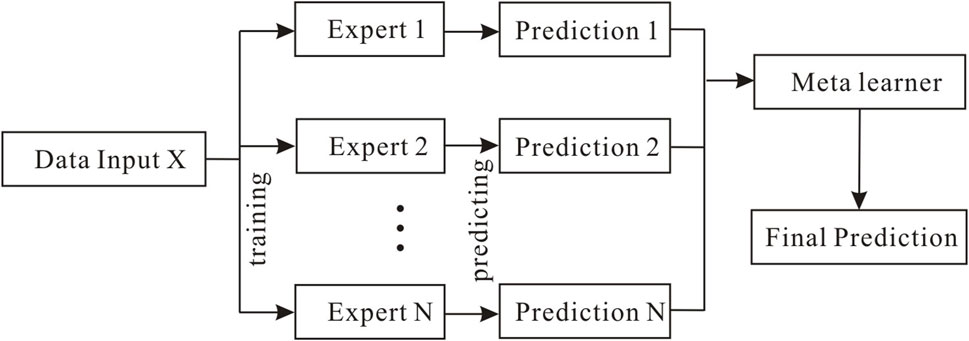
FIGURE 1. Stacking model architecture consisting of an input layer, experts, prediction results, meta-learner, and output layer.

In this study, the AdaBoost model (Freund and Schapire, 1997) is used as the meta-learner, and the weak learner in the model is a linear regression model. During the training process for each learner, the sample weight is adjusted according to the error rate of the previous round, and greater weights are assigned to the misclassified samples to iteratively learn and correct the errors, thereby improving the accuracy of the meta-learner model. The GNS model proposed in this study uses a gate network to assign different weights to the input data of the meta-learner and adds physical model constraints to allow the meta-learner to better find the best combination of expert models while complying with the physical model constraints.

2.4 Gate network

A gate network is a neural network structure that is used to control the flow and processing of information in a model. By adding a gate network mechanism, the input features can be selectively filtered, amplified, or suppressed, thus forming a constraint function for the model. In the classic stacking model, differences in expert performance cause the relationship between the features and learning objectives to become more complex. In addition, the impact of the added experts on the overall model cannot be measured. Therefore, this study introduces gate networks to solve the aforementioned problems, adjust the model architecture, and improve the accuracy and interpretability of the overall model.

In the GNS model, the role of the gate network includes three main aspects.

a. In the input layer, the gate network extracts the input petrophysical model and adds physical constraints to the input data of all expert models and meta-learners to improve the prediction performance and stability of the model and achieve model driving.

b. In the k-fold cross-validation of the expert model, the weight calculated according to the mean squared error (MSE) of each expert model is saved to the gate network, and the features corresponding to each expert model are weighted according to the weight combination saved by the gate network, which reduces the complexity of the meta-learner learning process and improves the robustness. The expert weights of the storage entry network are shown in Eq. 10, and the expert prediction results calculated based on the combination of weights are shown in Eq. 11.

${\mathit{w}}_{\mathit{t}\_\mathit{G}\mathit{N}}=\frac{\mathbf{1}}{\mathit{M}\mathit{S}{\mathit{E}}_{\mathit{t}}}/{\displaystyle \sum _{\mathit{i}=\mathbf{1}}^{\mathit{T}}}\frac{\mathbf{1}}{\mathit{M}\mathit{S}{\mathit{E}}_{\mathit{i}}}(10)$

where T is the total number of expert models, and $MS{E}_t$ is the MSE of the t-th expert.

${\mathit{H}}_{\mathit{t}}\left(\mathit{x}\right)={\mathit{w}}_{\mathit{t}\_\mathit{G}\mathit{N}}\cdot {\mathit{h}}_{\mathit{t}}\left(\mathit{x}\right)(11)$

where $h_t\left(x\right)$ is the prediction result of the t-th expert and $H_t\left(x\right)$ is the prediction result of the t-th expert after assigning weights through the gate network.

c. When the meta learner outputs results, the accuracy indicators of the expert model combination are evaluated through a gate network. Experts who have a positive impact on the accuracy indicators are retained, abandoning experts who have a negative impact on the accuracy indicators are abandoned to ensure that the overall performance of the model is improved.

2.5 GNS model architecture and workflow

For the formation permeability prediction problem, the aforementioned components are used in this study to form a GNS model. First, a dataset is created and labeled. The logging dataset includes the natural gamma-ray log (GR), spectral gamma-ray log (K-TH-U), compressional slow-ness log (DT), neutron log (CN), and density log (DEN). Lab-measured core permeability data points are used as labels. In addition to the logging data mentioned above, $V_{sh}$, $ND$, and ${\varphi }_D$, calculated using Eqs 6–9, are also input into the GNS, called petrophysical constraints. Finally, a petrophysical and data-driven intelligent model is developed.

In the input layer, the optimal combination of the corresponding well log curves is selected for each expert model based on the SHAP value, and the petrophysical constraints are input into the gate network. In the expert layer, petrophysical constraints are added to the input data of the expert model through the gate network, and the hyperparameters of the model are self-optimized. The Bayesian optimization method is used in this study to optimize the parameters; it estimates the posterior distribution of the objective function by constructing a Gaussian process (GP) model and determines the hyperparameter value for the next sampling, thereby quickly finding the global optimal solution. Cross-validation partitioning the dataset into multiple subsets, training the model on some of these subsets, and evaluating its performance on the remaining subsets. After model optimization is completed, each expert model is simulated and predicted using a five-fold cross-validation method. The performance of the expert model is evaluated according to the MSE of the model and stored in the gate network. Each expert model is then trained using all of the datasets.

According to the ranking of expert performance indicators, the expert model simulation prediction results are added to the meta-learner and given weights to form the input set of the meta-learner. At the same time, the gate network adds petrophysical constraints.

Finally, the meta-learner is trained. We evaluate the output results, retain the expert models that positively impact the overall model performance, eliminate the expert models that negatively impact the overall model, and finally output the prediction results of the best model combination.

Because the expert model adds dynamic weight constraints, it is more robust and interpretable than the classic stacking algorithm. Figure 2 shows the GNS workflow based on petrophysical and data-driven methods.

FIGURE 2

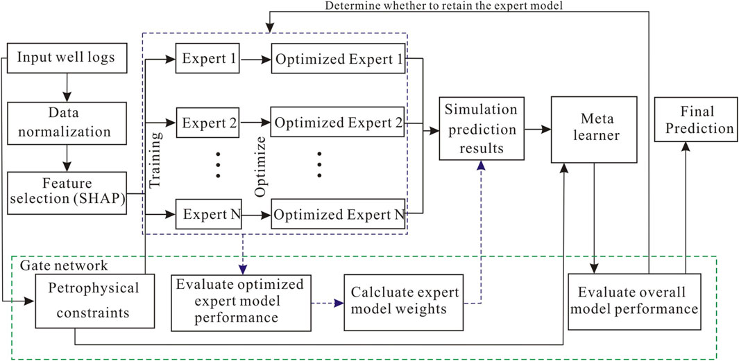
FIGURE 2. GNS model workflow consisting of five parts: the input layer, expert layer, meta-learner, gate network, and output layer.

2.6 Performance evaluation

To verify the reliability and accuracy of the proposed GNS model, three statistical parameters are introduced as performance evaluation indicators. The equations used to calculate each parameter are listed in Table 1.

TABLE 1

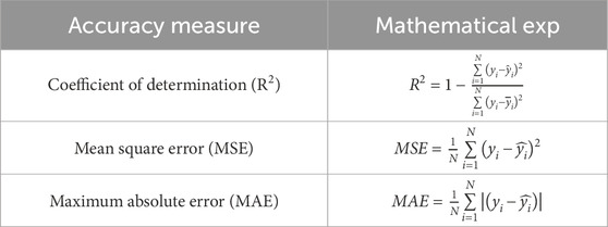
TABLE 1. Parameters for assessment to evaluate the model performance.

3 Case study

3.1 Geological background

The Dibei tight gas reservoir in the Kuqa Depression of the Tarim Basin has become a key exploration area because of its large gas reserve potential. The main production and storage unit is the Jurassic Ahe formation. The lithology is mainly coarse sandstone, and the sedimentary type is a braided river delta plain channel. The rock type in the sedimentation is mainly lithic sandstone, followed by feldspathic lithic sandstone, with a quartz content of more than 60%. Feldspar, clay minerals, calcite, and dolomite are all developed. The Dibei gas reservoir has low porosity, a complex pore throat structure, and a wide range of permeability changes. Multiple factors jointly control the permeability of the reservoir, and the predictive effect of the empirical model is poor. It is necessary to apply a model that can identify nonlinear characteristics between well logs and core data. Therefore, we apply the GNS model to predict the permeability.

3.2 Data acquisition

The stability and accuracy of the model depend on the reliability of the training data. In this study, 1,088 samples were collected from five wells in the Dibei area. The locations of the core wells are shown in Figure 3. The input variables include seven conventional well logs (GR, K, TH, U, DT, DEN, and CN) and three petrophysical constraints (ND, $V_{sh}$ , and ${\varphi }_D$); the permeability value is the desired output. To ensure that the GNS model has the best possible performance, the training data were normalized. Based on the data normalization, we calculated the SHAP value of each input feature, as shown in Figure 4, which reflects the contribution of each feature to the model prediction, further indicating the relative importance of each feature to the prediction results.

FIGURE 3

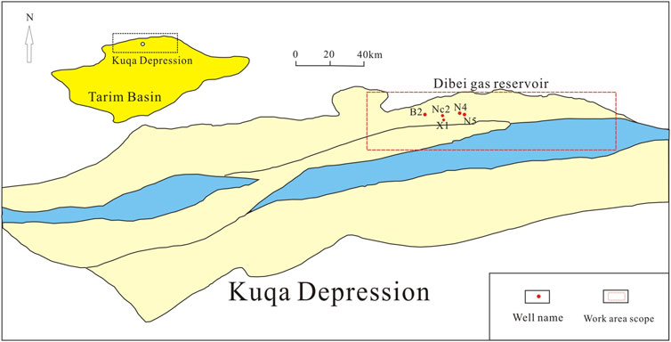
FIGURE 3. The Dibei gas reservoir is located in the northern part of the Kuqa Depression, as indicated by the red box in the thumbnail; the red dot indicates the location of the coring well.

FIGURE 4

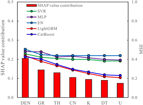
FIGURE 4. SHAP contribution of well logs and changes in the MSE of well log combinations in each expert model.

The bar chart in Figure 4 shows that the contributions of the SHAP values in descending order are DEN, GR, TH, CN, K, DT, and U. Five different expert models were trained based on the SHAP value contribution of the well log, and the MSE of the training results is shown in the line chart in Figure 4. The MSE reduction is defined as a log that has a positive contribution to the model, while conversely, when it has a negative contribution to the model, the positive contribution log is retained as the input of the expert model, and different log combinations are input for different expert models. Together with the permeability label, these constitute the training set, as summarized in Table 2.

TABLE 2

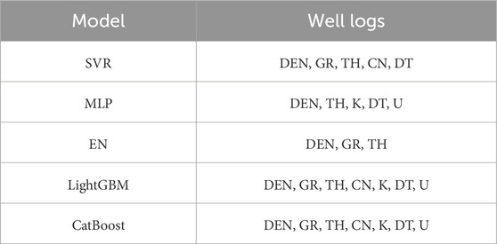
TABLE 2. Well log input combinations for different experts.

3.3 Model training and performance evaluation

The feature combinations in Table 2 are input into the expert model for training, and the Bayesian optimization method is used to find the optimal hyperparameter values such that the model can achieve the best performance on the target task. A performance comparison of the expert model using optimal hyperparameter values and the expert model using default parameters is summarized in Table 3.

TABLE 3

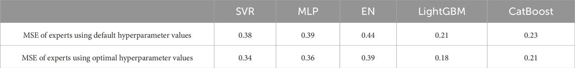
TABLE 3. Expert performance comparison when applying optimized and default hyperparameters.

The petrophysical constraints stored in the gate network are added to the feature combination of each expert to form the input dataset for each expert. Targeting the core permeability, multiple random sampling and no-replacement iterative predictions are conducted on experts to obtain a set of simulation prediction results, record the expert model MSE, save it to the gate network, and use all datasets to train each expert model. The expert combination is formed iteratively based on the MSE of the expert model (from small to large), the weight of each expert in the combination is calculated (Eq. 8), and the corresponding simulation prediction results are weighted (Eq. 9). Next, the weighted prediction results and petrophysical constraints are input into the meta-learner for training to determine the optimal expert model combination strategy. To demonstrate the effectiveness and advantages of the GNS algorithm, a classic stacking model is used for comparison. To ensure consistency, the same experts and meta-learners are used in the models. A performance comparison of the two models is shown in Figure 5.

FIGURE 5

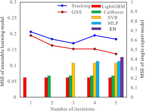
FIGURE 5. MSE of the expert model and changes in the MSE when iteratively inputting the ensemble learning model.

It can be seen that the addition of the gate network clearly improves the overall model. In contrast, the classic stacking model lacks petrophysical constraints and expert evaluation mechanisms and cannot optimize over-fitting, coupling correlation, and other problems existing in the integration process of experts; as a result, the overall performance of the stacking model is inferior to that of the GNS. For example, in the fourth iteration shown in Figure 5, the MLP model may have problems with dataset misfit or poor coupling with other expert results, resulting in negative improvements to the overall model when an expert is added to the stacking model. In the GNS algorithm, the addition of this expert is judged to be a negative improvement. Therefore, the prediction results of this expert are eliminated from the overall model, ultimately maintaining the quality of the overall expert group.

The above analysis shows that the performance of the GNS model is better than that of the stacking model, indicating that the improvement in the gate network is effective. To discuss the superiority of the model architecture, this study conducts a horizontal comparison with other ensemble learning models. We selected three representative integration strategies: two heterogeneous integration models (RCM and Voting) and a bagging integration model constructed using LightGBM. Three evaluation indicators—MSE, MAE, and R2—are used to evaluate the performance of the model. The results are summarized in Table 4. The GNS and RCM models have better prediction performance, and the GNS model achieves the best prediction results.

TABLE 4

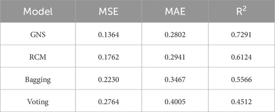
TABLE 4. Performance evaluation parameters of different ensemble learning models.

Figure 6A shows the error between the core permeability measured in the laboratory and that predicted using the GNS model. To compare the prediction effect more intuitively, the permeability is plotted on a cross diagram (Figure 6B), where the 45° diagonal line represents a perfect match between the predicted and true penetration rates. The prediction error of the model conforms to a normal distribution; therefore, the accuracy of the model can be judged based on the variance and MSE (Helle et al., 2001; Zhong et al., 2019). Figures 7–9 show the prediction results of the RCM, bagging, and voting models, respectively.

FIGURE 6

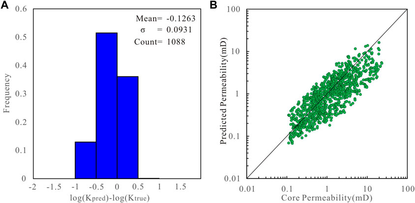
FIGURE 6. (A) Histogram of the error between the core measured permeability value and the permeability predicted by the GNS model. (B) Cross plot of the core measured permeability value and permeability predicted by the GNS model.

FIGURE 7

FIGURE 7. (A) Histogram of the error between the core measured permeability value and the permeability predicted by the RCM model. (B) Cross plot of the core measured permeability value and permeability predicted by the RCM model.

FIGURE 8

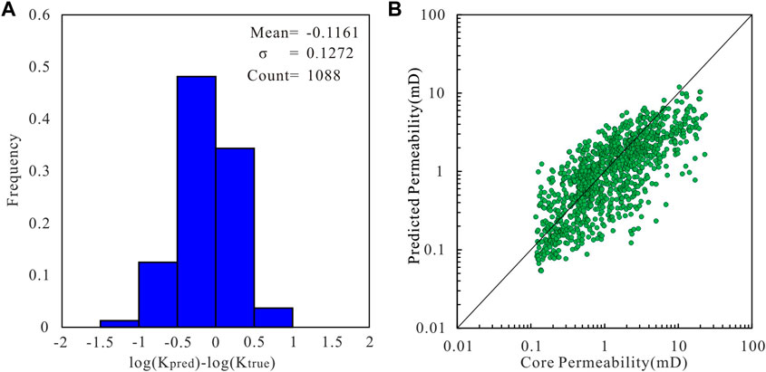
FIGURE 8. (A) Histogram of the error between the core measured permeability value and the permeability predicted by the bagging model. (B) Cross plot of the core measured permeability value and permeability predicted by the bagging model.

FIGURE 9

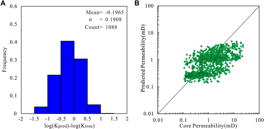
FIGURE 9. (A) Histogram of the error between the core measured permeability value and the permeability predicted by the voting model. (B) Cross plot of the core measured permeability value and permeability predicted by the voting model.

The GNS model has a variance of 0.0931 and MSE of 0.1364. It has the highest degree of fit with the core permeability values. The error does not exceed one order of magnitude for any of the core samples, showing the best performance (Figure 6). The variance of the RCM model is 0.1109 and the MSE is 0.1762. The prediction results are slightly lower in the high-permeability interval, and the performance is slightly weaker than that of the GNS (Figure 7). The variance of the bagging model is 0.1272, and the MSE is 0.2230. Some sample points exhibit large errors at different permeability intervals. This may be because random sampling will lead to a loss of some useful information (Figure 8). Finally, the voting model has the largest variance and MSE, and the predicted permeability has a larger error than the core permeability (Figure 9). These studies demonstrate that the GNS model is consistent with the measured permeability of the cores.

3.4 Prediction results

Well N4 is a core well in the Dibei gas reservoir in the Tarim Basin. The target reservoir is the Jurassic Ahe Formation. Logging data includes natural gamma ray log (GR), porosity logs (DEN-CN-DT), and natural gamma spectrum logs (K-TH-U). In this study, we selected the above seven well logs and three petrophysical constraints (VSH, PHID, and ND) as inputs, used the core permeability measured in the laboratory as label data, and entered it into the GNS model for prediction. For comparison, the results of several other ensemble learning models were obtained. Figure 10 shows the prediction results for each model in Well N4. The first track is the natural gamma curve, the second track is the natural gamma spectrum curve, the third track is the porosity log curve, and the fourth track is the petrophysical constraints. Tracks 6, 7, 8, and 9 are the comparisons between the prediction results of the GNS model, RCM model, bagging model, and voting model and the true value of the core permeability, respectively. The prediction results of the GNS model exhibit the best agreement with the core measurement results. The RCM and bagging models have certain errors at lower permeabilities. The voting model exhibits the largest difference from the core measurement results. The case study shows that the GNS model has advantages in predicting permeability. Importantly, we applied the gate network to integrate the petrophysical constraints with the model, rather than simply taking the petrophysical constraints as inputs. In addition, we controlled the weight of the model through the gate network, avoiding the influence of weak experts. Thus, the proposed model is more flexible than previously established empirical equations and other machine learning models.

FIGURE 10

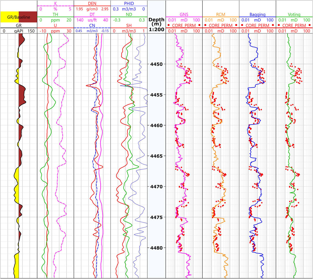
FIGURE 10. Permeability prediction results for Well N4 in the Dibei Gas Reservoir, Tarim Basin.

4 Discussion

In recent years, machine learning has promoted the intelligent development of log interpretation. In the process of supervised learning, machine learning automatically adjusts the internal structure to satisfy the mapping relationship between the feature data and label data and establishes a prediction model with certain generalization capabilities. However, data-driven learning is the core of current machine learning. Most studies have only considered the use of indicators such as accuracy and mean square error to evaluate the performance of machine learning models, ignoring the impact of physical constraints on the overall model. Therefore, even a model with superior performance is not convincing in its predictions for unknown samples. It is clear that a single data-driven method cannot meet the requirements of log interpretation tasks. The combination of model- and data-driven methods is a development trend for the future application of machine learning models in the field of log interpretation. This approach considers model performance and interpretability. While ensuring the accuracy of the model, it also ensures that it conforms to the physical laws of the logging interpretation process.

The stacking model typically consists of an expert model layer and a meta-learner, which has better performance than a single model in actual tasks. However, the meta-learner only learns the combination of experts and does not perform any evaluation or control of the experts, resulting in poor interpretability and difficulty in explaining the contribution of each model. The RCM model relies on the performance of experts, and some weak models may have a greater impact on the results and a weak ability to solve the problem of data imbalance. The bagging model aims to reduce the variance. When the data distribution was uneven, each basic model learned different features from different data subsets. In addition, if the basic model itself has overfitting or underfitting problems, bagging cannot solve them. The voting algorithm relies on the performance of experts. Because the weights are the same, the information obtained by each model may not be fully utilized. The voting model is sensitive to noise. In this study, it is also found that for sample sets with large differences in permeability, noise causes the model to obtain poor results. The GNS model controls the model through the gate network mechanism, adds petrophysical constraints to the inputs of the expert model and meta-learner, dynamically assigns weights to the output of the expert model, and finally iteratively evaluates the overall performance of the model. Connecting each training step of the model and adding constraints uniformly improves the shortcomings of the traditional model and significantly enhances the interpretability and credibility of the overall model.

However, petrophysical constraints are calculated from well logs, and there is still a certain similarity in their features. During the model training process, feature redundancy is possible, and the information dimension may not be sufficiently rich. Therefore, the choice of petrophysical constraints is important. In the future research, while applying petrophysical constraints, more logging information can be used as the input or constraint of the model, such as imaging logging to achieve better results.

5 Conclusion

This paper proposes a workflow for reservoir permeability prediction based on the GNS model. The SHAP value is used to analyze the contribution of the feature curve, select the optimal feature combination to build the traditional stacking model, and use the gate network to control and dynamically optimize the overall model. Finally, the results of other models are compared to verify the superior performance of the GNS model. The following conclusions can be drawn from this study.

1) The selection of a well log is crucial for the prediction performance of intelligent algorithms. Intelligent algorithms based on appropriate features can output more accurate results. SHAP contribution analysis is an effective means of evaluating the importance of well logs.

2) Based on the classical stacking model, the GNS model applies gate networks to control and dynamically optimize the overall model. GNS is an algorithm driven by both data and models. It retains the advantages of the stacking model’s strong expressive ability and significantly improves the interpretability of the algorithm. Compared with single data-driven algorithms, it is more reliable and superior in practical logging task applications.

3) The GNS model can effectively solve the nonlinear prediction problem of high-dimensional features. In the tight sandstone reservoir permeability prediction example, the results of the GNS model are closer to the laboratory-measured permeability than the results of the RCM, voting, and bagging models, thus verifying that the proposed model is an accurate method.

Data availability statement

The data analyzed in this study is subject to the following licenses/restrictions: exploratory research. Requests to access these datasets should be directed to PS, shipy0410@126.com.

Author contributions

PS: Conceptualization, Investigation, Methodology, Software, Validation, Writing–original draft, Writing–review and editing, Data curation, Formal Analysis. PS: Data curation, Methodology, Software, Validation, Writing–original draft, Writing–review and editing. KB: Validation, Writing–review and editing. CH: Validation, Writing–review and editing. XN: Validation, Writing–review and editing. ZM: Supervision, Validation, Writing–review and editing. PZ: Funding acquisition, Validation, Writing–review and editing, Supervision.

Funding

The author(s) declare financial support was received for the research, authorship, and/or publication of this article. The Science Foundation of China University of Petroleum, Beijing (2462020BJRC001).

Conflict of interest

Authors KB, CH and XN were employed by PetroChina Tarim Oilfield Company.

The remaining authors declare that the research was conducted in the absence of any commercial or financial relationships that could be construed as a potential conflict of interest.

Publisher’s note

All claims expressed in this article are solely those of the authors and do not necessarily represent those of their affiliated organizations, or those of the publisher, the editors and the reviewers. Any product that may be evaluated in this article, or claim that may be made by its manufacturer, is not guaranteed or endorsed by the publisher.

References

Ahmadi, M. A., Ebadi, M., Shokrollahi, A., and Majidi, S. M. J. (2013). Evolving artificial neural network and imperialist competitive algorithm for prediction oil flow rate of the reservoir. Appl. Soft Comput. 13 (2), 1085–1098. doi:10.1016/j.asoc.2012.10.009

CrossRef Full Text | Google Scholar

Ahmed, U., Crary, S., and Coates, G. (1991). Permeability estimation: the various sources and their interrelationships. J. Pet. Technol. 43 (5), 578–587. doi:10.2118/19604-PA

CrossRef Full Text | Google Scholar

Al-Anazi, A. F., and Gates, I. D. (2012). Support vector regression to predict porosity and permeability: effect of sample size. Comput. Geosci. 39, 64–76. doi:10.1016/j.cageo.2011.06.011

CrossRef Full Text | Google Scholar

Bai, Y., Tan, M., Shi, Y., Zhang, H., and Li, G. (2020). Regression committee machine and petrophysical model jointly driven parameters prediction from wireline logs in tight sandstone reservoirs. IEEE Trans. Geosci. Remote Sens. 60, 1–9. doi:10.1109/TGRS.2020.3041366

CrossRef Full Text | Google Scholar

Carman, P. C. (1937). Fluid flow through a granular bed. Trans. Instit. Chem. Eng. 15, 150–156. doi:10.1016/S0263-8762(97)80003-2

CrossRef Full Text | Google Scholar

Chen, C. H., and Lin, Z. S. (2006). A committee machine with empirical formulas for permeability prediction. Comput. Geosci. 32 (4), 485–496. doi:10.1016/j.cageo.2005.08.003

CrossRef Full Text | Google Scholar

Coates, G. R., and Dumanoir, J. L. (1973). “A new approach to improved log-derived permeability,” in SPWLA annual logging symposium (Lafayette, Louisiana: SPWLA).

Google Scholar

Freund, Y., and Schapire, R. E. (1997). A decision-theoretic generalization of on-line learning and an application to boosting. J. Comput. Syst. Sci. 55 (1), 119–139. doi:10.1006/jcss.1997.1504

CrossRef Full Text | Google Scholar

Friedman, J. H. (2001). Greedy function approximation: a gradient boosting machine. Ann. Stat. 29 (5), 1189–1232. doi:10.1214/aos/1013203451

CrossRef Full Text | Google Scholar

Helle, H. B., Bhatt, A., and Ursin, B. (2001). Porosity and permeability prediction from wireline logs using artificial neural networks: a North Sea case study. Geophys. Prospect. 49 (4), 431–444. doi:10.1046/j.1365-2478.2001.00271.x

CrossRef Full Text | Google Scholar

Jamialahmadi, M., and Javadpour, F. (2000). Relationship of permeability, porosity and depth using an artificial neural network. J. Pet. Sci. Eng. 26 (1-4), 235–239. doi:10.1016/S0920-4105(00)00037-1

CrossRef Full Text | Google Scholar

Kalule, R., Abderrahmane, H. A., Alameri, W., and Sassi, M. (2023). Stacked ensemble machine learning for porosity and absolute permeability prediction of carbonate rock plugs. Sci. Rep. 13 (1), 9855. doi:10.1038/s41598-023-36096-2

PubMed Abstract | CrossRef Full Text | Google Scholar

Karimpouli, S., Fathianpour, N., and Roohi, J. (2010). A new approach to improve neural networks' algorithm in permeability prediction of petroleum reservoirs using supervised committee machine neural network (SCMNN). J. Pet. Sci. Eng. 73 (3-4), 227–232. doi:10.1016/j.petrol.2010.07.003

CrossRef Full Text | Google Scholar

Kozeny, J. (1927). Uber kapillare leitung der Wasser in boden. R. Acad. Sci. 136, 271–306.

Google Scholar

Lundberg, S., and Lee, S. I. (2016). An unexpected unity among methods for interpreting model predictions. arXiv Preprint. doi:10.48550/arXiv.1611.07478

CrossRef Full Text | Google Scholar

Lundberg, S. M., Erion, G., Chen, H., Degrave, A., Prutkin, J. M., Nair, B., et al. (2020). From local explanations to global understanding with explainable AI for trees. Nat. Mach. Intell. 2 (1), 56–67. doi:10.1038/s42256-019-0138-9

PubMed Abstract | CrossRef Full Text | Google Scholar

Lundberg, S. M., Erion, G. G., and Lee, S. I. (2018). Consistent individualized feature attribution for tree ensembles. arXiv Preprint. doi:10.48550/arXiv.1802.03888

CrossRef Full Text | Google Scholar

Lundberg, S. M., and Lee, S. I. (2017). “A unified approach to interpreting model predictions,” in NIPS'17: proceedings of the 31st international conference on neural information processing systems (ACM). Available at: https://www.aap.org/sections/perinatal/NCE08/TheRole2.pdf

Google Scholar

Matinkia, M., Hashami, R., Mehrad, M., Hajsaeedi, M. R., and Velayati, A. (2023). Prediction of permeability from well logs using a new hybrid machine learning algorithm. Petroleum 9 (1), 108–123. doi:10.1016/j.petlm.2022.03.003

CrossRef Full Text | Google Scholar

Mauran, S., Rigaud, L., and Coudevylle, O. (2001). Application of the carman–kozeny correlation to a high-porosity and anisotropic consolidated medium: the compressed expanded natural graphite. Transp. Porous Med. 43 (2), 355–376. doi:10.1023/a:1010735118136

CrossRef Full Text | Google Scholar

Mohaghegh, S., and Ameri, S. (1995). Artificial neural network as a valuable tool for petroleum engineers. Paper SPE, 29220, 1–6.

Nazari, S., Kuzma, H. A., and Rector, J. W. (2011). “Predicting permeability from well log data and core measurements using support vector machines,” in SEG technical program expanded abstracts 2011. Editor S. Fomel (Tulsa, Okla: Society of Exploration Geophysicists). doi:10.1190/1.3627601

CrossRef Full Text | Google Scholar

Nilsson, N. J. (1965). Learning machines. New York: McGraw-Hill.

Google Scholar

Paterson, M. (1983). The equivalent channel model for permeability and resistivity in fluid-saturated rock—a re-appraisal. Mech. Mat. 2 (4), 345–352. doi:10.1016/0167-6636(83)90025-X

CrossRef Full Text | Google Scholar

Rogers, S., Chen, H., Kopaska-Merkel, D. T., and Fang, J. (1995). Predicting permeability from porosity using artificial neural networks. AAPG Bull. 79 (12), 1786–1797. doi:10.1306/7834DEFE-1721-11D7-8645000102C1865D

CrossRef Full Text | Google Scholar

Saemi, M., Ahmadi, M., and Varjani, A. Y. (2007). Design of neural networks using genetic algorithm for the permeability estimation of the reservoir. J. Pet. Sci. Eng. 59 (1-2), 97–105. doi:10.1016/j.petrol.2007.03.007

CrossRef Full Text | Google Scholar

Saljooghi, B. S., and Hezarkhani, A. (2014). Comparison of WAVENET and ANN for predicting the porosity obtained from well log data. J. Pet. Sci. Eng. 123, 172–182. doi:10.1016/j.petrol.2014.08.025

CrossRef Full Text | Google Scholar

Sammut, C., and Webb, G. I. (2011). Encyclopedia of machine learning. Berlin: Springer Science & Business Media.

Google Scholar

Timur, A. (1968). “An investigation of permeability, porosity, and residual water saturation relationships,” in SPWLA 9th annual logging symposium (New Orleans, Louisiana: SPWLA).

Google Scholar

Wolpert, D. H. (1992). Stacked generalization. Neural Netw. 5 (2), 241–259. doi:10.1016/S0893-6080(05)80023-1

CrossRef Full Text | Google Scholar

Wu, T. (2004). Permeability prediction and drainage capillary pressure simulation in sandstone reservoirs. Doctoral thesis. Texas: Texas A&M University.

Google Scholar

Zhang, G., Wang, Z., Mohaghegh, S., Lin, C., Sun, Y., and Pei, S. (2021). Pattern visualization and understanding of machine learning models for permeability prediction in tight sandstone reservoirs. J. Pet. Sci. Eng. 200, 108142. doi:10.1016/j.petrol.2020.108142

CrossRef Full Text | Google Scholar

Zhang, H., Fu, K., Lv, Z., Wang, Z., Shi, J., Yu, H., et al. (2022a). FTCN: a reservoir parameter prediction method based on a fusional temporal convolutional network. Energies 15 (15), 5680. doi:10.3390/en15155680

CrossRef Full Text | Google Scholar

Zhang, S., Gu, Y., Gao, Y., Wang, X., Zhang, D., and Zhou, L. (2022b). Petrophysical regression regarding porosity, permeability, and water saturation driven by logging-based ensemble and transfer learnings: a case study of sandy-mud reservoirs. Geofluids 2022, 1–31. doi:10.1155/2022/9443955

CrossRef Full Text | Google Scholar

Zhong, Z., Carr, T. R., Wu, X., and Wang, G. (2019). Application of a convolutional neural network in permeability prediction: a case study in the Jacksonburg-Stringtown oil field, West Virginia, USA. Geophysics 84 (6), B363–B373. doi:10.1190/geo2018-0588.1

CrossRef Full Text | Google Scholar

Zhu, L. Q., Zhang, C., Wei, Y., and Zhang, C. M. (2017). Permeability prediction of the tight sandstone reservoirs using hybrid intelligent algorithm and nuclear magnetic resonance logging data. Arab. J. Sci. Eng. 42 (4), 1643–1654. doi:10.1007/s13369-016-2365-2

CrossRef Full Text | Google Scholar