Dispersion and fate of methane emissions from cold seeps on Hikurangi Margin, New Zealand

The influence of cold seep methane on the surrounding benthos is well-documented but the fate of dissolved methane and its impact on water column biogeochemistry remains less understood. To address this, the distribution of dissolved methane was determined around three seeps on the south-east Hikurangi Margin, south-east of New Zealand, by combining data from discrete water column sampling and a towed methane sensor. Integrating this with bottom water current flow data in a dynamic Gerris model determined an annual methane flux of 3 x 10⁵ kg at the main seep. This source was then applied in a Regional Ocean Modelling System (ROMS) simulation to visualize lateral transport of the dissolved methane plume, which dispersed over ∼100 km in bottom water within 1 year. Extrapolation of this approach to four other regional seeps identified a combined plume volume of 3,500 km³ and annual methane emission of 0.4–3.2 x 10⁶ kg CH₄ y^-1. This suggests a regional methane flux of 1.1–10.9 x 10⁷ kg CH₄ y^-1 for the entire Hikurangi Margin, which is lower than previous hydroacoustic estimates. Carbon stable isotope values in dissolved methane indicated that lateral mixing was the primary determinant of methane in bottom water, with potential methane oxidation rates orders of magnitude lower than the dilution rate. Calculations indicate that oxidation of the annual total methane emitted from the five seeps would not significantly alter bottom water dissolved carbon dioxide, oxygen or pH; however, superimposition of methane plumes from different seeps, which was evident in the ROMS simulation, may have localized impacts. These findings highlight the value of characterizing methane release from multiple seeps within a hydrodynamic model framework to determine the biogeochemical impact, climate feedbacks and connectivity of cold seeps on continental shelf margins.

1 Introduction

Although the ocean only accounts for 1%–3% of global methane (CH₄) emissions (9–22 Tg CH₄ y⁻¹, Saunois et al., 2020) marine methane is attracting increasing attention, in part due to its sensitivity to climate change. Marine methane sources are dominated by cold seeps on continental shelf margins and coasts (Weber et al., 2019), which primarily originate from underlying gas hydrates. The latter form in the Gas Hydrate Stability Zone (GHSZ), at low temperature and high pressure, hence their subsurface presence on continental shelves and margins (Hester and Brewer, 2009). Estimates vary widely and indicate that 450–75,000 Pg CH₄ may be stored globally in these reservoirs (Klauda and Sandler, 2005; Wallmann et al., 2012), with annual global seafloor seepage potentially reaching 65 Tg (US EPA: Office of Atmospheric Programs, 2010). However, their contribution to atmospheric emissions is negligible (Saunois et al., 2020), due to a combination of physical, geological and biological barriers that minimize methane transfer to the ocean surface. Methane flux from subsurface hydrates is primarily suppressed by anaerobic methanotrophy in the overlying sediment, which significantly reduces methane release into bottom water to ∼0.02 Gt C y⁻¹ (Boetius and Wenzhöfer, 2013). However, gaseous methane can evade this benthic filter (Sommer et al., 2006), with bubble ebullition and subsequent diffusion elevating dissolved methane in bottom waters (McGinnis et al., 2006). Dispersion and dilution by bottom currents (Kessler et al., 2011; Steinle et al., 2015), and oxidation via the pelagic filter of aerobic methanotrophs (Reeburgh, 2007) then further reduce dissolved methane concentration (de Angelis et al., 1993; Mau et al., 2013; Leonte et al., 2017). The dominance of lateral flow relative to vertical exchange in bottom and intermediate waters, combined with stratification in the main pycnocline, effectively caps the transfer of dissolved methane to surface waters and the atmosphere, with retention in deeper water ultimately resulting in aerobic oxidation to carbon dioxide (CO₂) (Valentine et al., 2001; Reeburgh, 2007).

Methane release at cold seeps has a significant influence on local benthic biology, as it supports microbial communities and associated biogeochemical pathways that sustain unique infauna and macrofauna assemblages via chemosynthesis (Boetius and Wenzhöfer, 2013; Bowden et al., 2013). There is also evidence around seep sites of trophic transfer of carbon derived from methane in food webs that include commercially important fisheries species (Niemann et al., 2013; Seabrook et al., 2019). The potential sensitivity of hydrates to tectonic activity (Crutchley et al., 2023; Rudebusch et al., 2023) and ocean warming (Ruppel and Kessler, 2017), and also interest in methane hydrates as a potential fuel source (Moridis et al., 2011), has focused attention on the fate of methane in bottom water. Warming of deep water may destabilize hydrates at the upper edge of the GHSZ, as indicated in the paleorecord by significant methane release from subsurface reservoirs coincident with periods of ocean warming (Maslin et al., 2010), and there is increasing contemporary evidence for this (Phrampus and Hornbach, 2012; Trivedi et al., 2022). The resulting increase in methane in deep waters could enhance CO₂ production and consumption of oxygen (O₂) via aerobic oxidation, so accelerating acidification and deoxygenation (Biastoch et al., 2011; Ruppel, 2011; Boudreau et al., 2015). However, the impact of seep methane on water column biogeochemistry has received less attention (Levin et al., 2016), in part due to the challenge of tracking dissolved methane in bottom water.

Fluid seepage and cold seeps are well-characterized along the Hikurangi Margin, east of New Zealand (Lewis and Marshall, 1996; Barnes et al., 2010; Watson et al., 2020), with subsurface hydrates evident as bottom-simulating reflectors in seismic data (Henrys et al., 2003; Klaucke et al., 2010; Crutchley et al., 2021; Crutchley et al., 2023). Regional analysis indicates seepage occurring predominantly along the deforming backstop of the margin, with fluid release from both the subducting plate and the accretionary wedge (Watson et al., 2020). Fluid migration is facilitated by folding, fractures and faults arising from tectonic activity and strata of elevated permeability and porosity. Cold seep location is further evidenced by the presence of gas flares or bubble plumes in hydroacoustic backscatter data (Turco et al., 2022), that may extend up to 1 km above the seafloor (Faure et al., 2010; Law et al., 2010). To determine the fate of methane released from cold seeps, dissolved methane concentrations and related biogeochemical parameters including dissolved O₂ and carbonate system parameters were measured in the water column at three seep sites on the south-east Hikurangi Margin. As tracking of dissolved methane in bottom waters is confounded by tidal currents and dispersal in three dimensions, the dissolved methane source and distribution at the main seep site was simulated at local scales in a hydrodynamic framework using a dynamic Gerris model, with dispersal along the margin then determined using the Regional Ocean Modelling System (ROMS). This was extended to four other regional seeps (Turco et al., 2022) to assess the combined dispersal of seep methane and influence on bottom water biogeochemistry. Methane loss was assessed by potential oxidation rate measurements, with oxidation also examined indirectly using carbon stable isotope values in dissolved methane (δ¹³C-CH₄), to establish the relative influence of dispersion and oxidation on seep methane in bottom waters along the Hikurangi Margin.

2 Methods

2.1 Regional setting

Sampling was carried out during July 2019 onboard R/V Tangaroa, as part of the New Zealand HYDEE (Gas Hydrates: Economic Opportunities and Environmental Implications) programme. The study area lies at the southern end of the Hikurangi subduction margin (Figure 1) where the Pacific Plate subducts obliquely beneath the Australian Plate. Measurements were focused on three seeps - Maungaroa, Glendhu Ridge and Uruti Ridge - with data from two additional seep sites–Pahaua Bank and Uruti Ridge West - also considered in the analysis (Turco et al., 2022; see Table 1). Dispersal modelling focused on the main seep site at Maungaroa, where a subsurface layer of gas of >200 m height below the GHSZ has generated doming, fracturing and formation of a conduit that facilitates gas transfer to the seafloor (Crutchley et al., 2021).

Figure 1

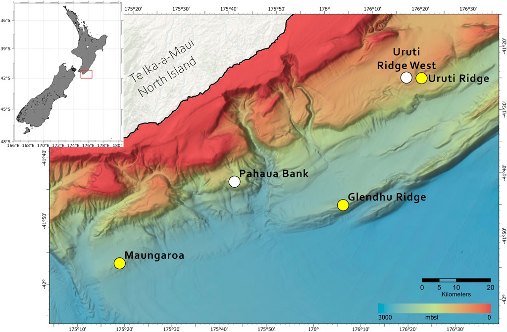
Figure 1. Location of the five seep sites on the south-east Hikurangi Margin plotted against bathymetric depth (m), as shown in the colour bar. The three seep sites surveyed in this study (Maungaroa, Uruti Ridge and Glendhu Ridge) are indicated by yellow circles, and the two additional sites (Uruti Ridge West and Pahaua Bank, (Turco et al., 2022) by white circles. The x-axis shows longitude (ºEast) and y-axis latitude (ºSouth).

Table 1

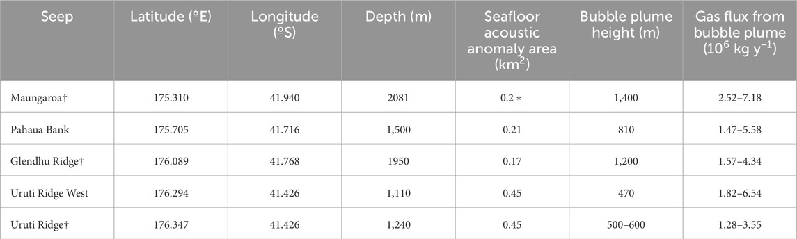
Table 1. Seep locations and dimensions on the south-east Hikurangi Margin (all data from Turco et al., 2022, except for * Crutchley et al., 2021), with the sites sampled in this study indicated by †.

2.2 Bottom water hydrography and properties

A seafloor mooring was deployed in the vicinity of each of the three seeps consecutively to record bottom water physical and biogeochemical properties. The mooring frame was attached to a 460 kg ballast weight and supported a 600 kHz Acoustic Doppler Current Profiler (ADCP) for measuring current direction and velocity. A SBE 37 ODO MicroCAT with conductivity, temperature and optical dissolved O₂ sensors was also deployed on the mooring at ∼15 m above the seafloor. The mooring was deployed for periods of 3–5 days at each site, which either preceded or followed other sampling activities to ensure the mooring and sensors were not compromised. On recovery, the mooring frame was decoupled from the ballast by remote activation of an acoustic release device whilst the ballast remained on the seafloor. The ADCP data was processed and quality controlled to generate a filtered data set with records at 120 s intervals over the lifetime of each respective deployment.

2.3 Water column sampling and characterisation

Dissolved methane concentrations were determined by four different approaches: discrete water sample collection in Niskin bottles on a CTD (Conductivity, Temperature and Depth) rosette in either a) standard vertical profiling mode or b) lateral towed mode, with methane concentration also measured by a methane sensor deployed on c) the CTD or d) a Deep Towed Imaging System (DTIS, Bowden et al., 2013). As the dissolved methane plume was largely retained in near-bottom waters, the CTD and DTIS lateral tows focused on the bottom 10 m of water overlying the seafloor, with each sensor tow orientated relative to the seep by reference to a predetermined location and information from preceding tows. Each sensor tow started ∼1 km from the seep and crossed this at the transect mid-point before completion at a similar distance of 1 km. During the CTD sensor tow, Niskin bottle water samples were obtained with increased sampling frequency close to the seep, with the remaining bottles fired in the bottom 200–500 m during retrieval. At least one vertical CTD cast was carried out at a distance of >1 km from the seep at all three sites to characterize background conditions. Bottom waters at Maungaroa received the most intense sampling, with six DTIS tows and 12 CTDs. Stratification was determined using buoyancy frequency squared (N²), which was calculated as:

${\mathrm{N}}^2=g/{\rho }_{0.}\delta \rho /\rho z$

where g is gravitational acceleration, ρ₀ is a reference density, and δρ/ρz is the vertical density gradient (Stevens et al., 2012).

2.4 Dissolved methane measurements

2.4.1 Analysis of discrete water samples

Seawater from the 10-L Niskin bottles was sub-sampled into 240 mL glass serum bottles, which were overflowed by at least 100% to exclude bubbles and then sealed with butyl rubber septa. The samples warmed passively to ambient temperature, with analysis within 4–5 h of collection. A 40 mL headspace of O₂-free nitrogen (N₂) was injected into the bottle whilst 40 mL of seawater was expelled, with the two phases subsequently equilibrated at room temperature for 30 min. The equilibrated headspace was displaced through a drying tube containing magnesium perchlorate and then a 2.9 mL sample loop, the contents of which were injected onto a 1/8” molecular sieve chromatographic column with methane detection by a Flame Ionisation Detector (Law et al., 2010). Calibration was carried out using prepared gas standards certified by comparison in an international calibration exercise (Wilson et al., 2018), with peak area variation of <0.35% over a 12-h analysis period. Dissolved methane concentration (nmol L⁻¹) was calculated from the measured partial pressure of methane in the headspace, following correction for water vapour and using the equilibration temperature and salinity with the solubility coefficients of Weisenburg and Guinasso (1979). Precision of duplicate sample analysis was 2.5% (1 standard deviation), consistent with the reproducibility reported in an international intercomparison (Wilson et al., 2018). Methane saturation from atmospheric equilibrium was calculated using the mean atmospheric methane mixing ratio of 1740 ppb recorded at the nearby National Institute of Water and Atmospheric Research (NIWA) Baring Head Global Atmosphere Watch Programme station (World Data Centre for Greenhouse Gases; kishou.go.jp), with dissolved methane concentration expressed as a percentage of expected saturation. An example of the vertical profile data for dissolved methane and associated parameters is available in Supplementary Table S1 (Supplementary Material), with the data for all profiles available at the associated website.

2.4.2 Continuous dissolved methane measurement

The dissolved methane dataset was extended to greater temporal and spatial resolution by deployment of a METS Sensor (Franatech, Oslo, Norway). This sensor was used in two modes: i) attached to the CTD, which enabled comparison with discrete sample data so enabling sensor calibration at in situ temperature and pressure; and ii) mounted on the DTIS (Bowden et al., 2013), which generated detailed transects across the seep region in bottom waters between 2 and 8 m above the seafloor. Each CTD lateral tow was at slightly shallower depths (5–15 m above the seabed), with the CTD initially held for 5–10 min to allow equilibration of the METS sensor before towing commenced. The METS relies upon methane diffusion across a permeable membrane, with diffusion assisted by a pump head, and detection by semi-conductor technology. Methane adsorption results in a change in conductivity which is converted to voltage as an output signal, with temperature sensitivity accounted for by a separate voltage (Krabbenhoefft et al., 2010). As diffusion across the membrane is rate-limiting this results in a lag in METS response, which was corrected for by comparison with in situ discrete sample data. The METS working temperature minimum of +2°C and methane concentration sensitivity of ∼1 nmol L^-1 were well suited to measurements in bottom waters along the Hikurangi Margin.

2.5 Dissolved inorganic carbon and total alkalinity

Bottom water collected in the Niskin bottles was subsampled into 1-L and 2-L glass bottles on selected CTD tows and profiles at seep and background stations for analysis of dissolved inorganic carbon (DIC) and total alkalinity (TA), respectively. The bottles were overflowed by 100%, with samples preserved by saturated mercuric chloride addition, sealed with parafilm and stored in the dark, with subsequent analysis in the laboratory. DIC concentration was determined coulometrically (Dickson et al., 2007) with an estimated accuracy and precision of ±1 μmol kg^–1 based on repeat analysis of Dickson Certified Reference Materials. TA was determined by closed-cell potentiometric titration (Dickson et al., 2007), using a curve-fitting optimization with least squares analysis of the titration curve, with an estimated accuracy and precision ±2 μmol kg^–1 also based on repeat analysis of Dickson Certified Reference Materials measurements. The DIC and TA data were used to calculate in situ pH on the total scale using in situ temperature, salinity and pressure and Mehrbach dissociation constants (Mehrbach et al., 1973), as refitted by Dickson and Millero (1987).

2.6 Dissolved methane carbon isotope analysis

Stable C isotope ratios of CO₂ were measured using a GasBench II and GC-PAL autosampler coupled to a DELTA V Plus isotope ratio mass spectrometer (IRMS) (all Thermo Fisher Scientific, Bremen, Germany). Daily checks confirmed that IRMS linearity was <0.06‰ volt⁻¹ for a known m/z 44 voltage span, and the standard deviation of δ¹³C values from 10 peaks of working standard CO₂ was always <0.06‰. Values of sample δ¹³C were derived relative to the CO₂ working standard gas introduced directly into the IRMS and corrected for ¹⁷O (Santrock et al., 1985) by Isodat software (version 3.0.94.17; Thermo Fisher Scientific, Bremen, Germany). Isotopic values were reported in δ-notation relative to the Vienna Pee Dee Belemnite scale. This approach was used for both dissolved methane (Section 2.6.1), and also for DIC in the potential oxidation rate measurement (Section 2.7).

2.6.1 Sample preparation for methane carbon isotope analysis

Seawater samples for dissolved δ¹³C-CH₄ analysis were subsampled from the Niskin bottles into 285 mL glass serum bottles, poisoned with mercuric chloride and sealed with butyl rubber septa. Sample temperature was slowly raised to ambient temperature with a hypodermic needle inserted through the septa to allow water to expel during volume change. In the laboratory, a 15 mL headspace of ultra-high purity helium was introduced while withdrawing an equivalent volume of seawater to obtain a seawater:headspace volume ratio of 18, with the two phases equilibrated on a shaker for 30 min. Using a GasBench II and GC PAL autosampler (Thermo Fisher Scientific, Bremen, Germany) the headspace gas was purged at 20 mL min⁻¹ in a helium carrier flow and directed through a series of in-line traps to remove water, carbon monoxide and CO₂. A PreCon cold trap immersed in liquid N₂ removed nitrous oxide before sample methane was trapped on a second PreCon automated cold trap comprised of 100 cm of coiled GS-Q capillary column (divinylbenzene (DVB), wide-bore 0.32 mm D; Agilent Technologies, United States) also held in liquid N₂ (Yarnes, 2013). On removal of the second trap from the liquid N₂ the methane was transferred into the helium carrier flow and combusted by passing through the PreCon combustion reactor (99.8% alumina, 1.6 mm outer diameter, 0.8 mm bore, 327 mm length; McDanel Ceramics, United States) at 1,000°C. After drying, the CO₂ produced by methane combustion was cryo-focused in the GasBench II cold trap held in liquid N_2, and then separated from residual gases by a chromatographic column (CP-PoraPLOT Q) at 70°C. C stable isotope analysis was as described above, with δ¹³C-CH₄ from clean air from the Baring Head station used to correct sample δ¹³C-CH₄ values (Paul et al., 2007).

2.7 Methane oxidation rate

Potential methane oxidation rate was measured in selected bottom water samples using ¹³C-CH₄ addition, following the method of Leonte et al. (2017). Seawater was transferred from the Niskin bottle into 6 x 240 mL serum bottles for each depth sample, sealed with butyl rubber septa and aluminium seals, and placed in the dark at ambient bottom water temperature (2–2.5°C). Within three-five hours, four of the six serum bottles were injected with 50 µL ¹³C-CH₄ mixed with 50 µL ambient air from a gas-tight syringe, during which the serum bottle was inverted and the rubber seal perforated by a separate needle to maintain atmospheric pressure in the bottle. The remaining two serum bottles were not amended and provided a time zero for the rate measurement. All bottles were gently agitated for 20 min on a wrist-action shaker, after which the four amended samples were incubated in the dark at ambient bottom water temperature for three-five days. The incubation was terminated at time zero, Day 2 and Day 4 by removal of 2 mL of water; this was injected into a 12 mL gas-tight glass vial sealed with a rubber septum previously flushed with high purity helium and containing 100 µL of phosphoric acid. In the laboratory, acidified samples were equilibrated overnight at 24°C, during which the CO₂ released by acidification of DIC had equilibrated with the headspace. C stable isotope analysis was as described above in Section 2.6. Reference materials IAEA NBS-18 and IAEA-603 were used to normalize all δ¹³C_gas values (Paul et al., 2007). Values of δ¹³C-DIC were calculated from δ¹³C_gas values by accounting for the C stable isotope fractionation associated with the CO₂ gas-aqueous partition (Assayag et al., 2006). Potential methane oxidation rate was determined by the transfer of ¹³C from the methane gas to DIC. Background in situ DIC concentrations were determined using the individual sample CO₂ peak values generated by the GasBench II, calibrated against a subset of samples analysed by coulometry, as detailed in Section 2.5. Rates (nmol l⁻¹ d⁻¹, hereafter identified as nM d⁻¹) were derived using the approach of Leonte et al. (2017), and are regarded as “potential” oxidation, reflecting the large ¹³C-CH₄ addition relative to the background dissolved methane concentration.

2.8 Modelling

2.8.1 Near-field dispersion of dissolved methane in bottom water

A dynamic model of nearfield dispersion of dissolved methane around the Maungaroa seep was developed using Gerris, a semi-structured adaptive grid model for the solution of the non-hydrostatic Navier–Stokes equations (S. Popinet, http://gfs.sf.net; Rickard, 2020). The primary aim of the Gerris modelling was to estimate the source input of methane into the water column by assessing advection and diffusion of the methane tracer via fitting to the spatial and temporal transect observations. Dissolved methane was treated as a passive tracer and so was advected and diffused with the imposed flow. As Gerris is applicable to small scales it was appropriate for modelling dispersion of dissolved methane within a 1 km radius of the seep where most of the water sampling took place. The three-dimensional model domain spanned 2.25 km in each horizontal direction and 250 m in the vertical plane, with grid spacing over most of the domain of 7.8 m. The model incorporated advection associated with M2 tidal currents, as measured by the ADCP, with the seep methane assumed to be entrained within 50 m above the seafloor (see Results). The model was spun up for a number of M2 tidal cycles, thereby allowing the methane tracer to advect and diffuse across the domain, with two to four M2 tidal cycles producing tracer patterns that best fitted the observations. Using these best fits an “optimal” ratio of the observed maximum methane concentration to the Gerris model maximum was determined for each transect and profile, with the average ratio subsequently used to calculate methane emission.

2.8.2 Far-field dispersion of dissolved methane

The ROMS (Haidvogel et al., 2008) was used to simulate the advection of passive ‘dye’ tracers released at each of the five seep sites (Table 1) along the southern Hikurangi Margin over a period of 1 year. The model domain spans the continental shelf of the eastern North Island of New Zealand, from Cook Strait in the south to East Cape in the North, with a horizontal resolution of 2 km and 30 terrain-following vertical coordinates. The model bathymetry was constructed from various sources including the NIWA gridded bathymetry database, land elevation data, regional coastline data, and the General Bathymetric Chart of the Oceans (GEBCO) gridded ocean bathymetry. The model was initialized on 1 January 2013 with initial and boundary conditions derived from a global ocean reanalysis based on the Hybrid Coordinate Ocean Model (HYCOM; Chassignet et al., 2009). The global HYCOM product used provides daily snapshots of the 3-dimensional state of the global ocean on a 1/12° grid. Tidal currents were added to the HYCOM boundary conditions using amplitude and phase data for 13 tidal constituents derived from the New Zealand tidal model described by Walters et al. (2001). The ROMS simulation was forced at the surface with wind stress calculated from 3-hourly winds obtained from the 12 km New Zealand Limited Area Model (NZLAM; Lane et al., 2009). Heat and freshwater fluxes were obtained from six-hourly NCEP/NCAR reanalysis data with a horizonal resolution of 2.5° (Kalnay et al., 1996).

The passive tracer computational capabilities of ROMS were used to determine the dispersal of methane via a conservative dye tracer released in the bottom three grid cells (150–200 m above the bottom) at each of the five seep sites. The passive tracers were advected from the release locations following the same governing equations as temperature and salinity. The passive tracer has a unit concentration and was initialized from each location with a value of 100. To simulate a continuous release, the passive tracers were nudged back to a value of 100 at the release locations on a daily basis using a nudging coefficient of 0.05 days⁻¹.

The calculated methane source function generated by the Gerris model was applied to the ROMS dye tracer to determine dispersion from the Maungaroa seep in bottom waters along the Hikurangi Margin. The ratio of the Gerris source function to an independent estimate of methane emission from hydroacoustic backscatter (Turco et al., 2022) was generated for Maungaroa, and then applied to the estimated methane emission from hydroacoustic backscatter for the other four sites (Turco et al., 2022) to re-evaluate the total emission from the five seeps.

3 Results

3.1 Dissolved methane distribution

Analysis of the integrated discrete water sample and high-resolution sensor data determined that most of the dissolved methane was retained in bottom waters up to 200 m above the seafloor, although this was biased by the large number of sensor measurements obtained within 5 m of the seafloor. Dissolved methane concentration varied over four orders of magnitude, with maximum concentrations exceeding 2 μmol L^-1 (supersaturation of 60,000 relative to atmospheric methane) at the Maungaroa and Uruti Ridge sites (Figure 2, Supplementary Table S1). The lower dissolved methane maximum at Glendhu Ridge may reflect that this site is characterized by a number of smaller dispersed seeps (Turco et al., 2022). All three sites showed methane undersaturation, indicative of methane oxidation, in the mid-water column at depths of 750–1,000 m for the shallower Uruti Ridge site and 1,000–1,500 m for the two deeper sites (Figure 2; Supplementary Table S1). Mid-water column methane concentrations were similar at the background and seep stations at Maungaroa, although elevated methane concentration of ∼20 nmol L^-1 was evident at 1,600–1800 m at the background sites. All three sites exhibited a mean methane concentration of ∼4.5 nmol L⁻¹ between 500 m and the surface, with a maximum of ∼12.5 nmol L⁻¹ at a background site near Maungaroa. The near-surface methane supersaturation of <150% was consistent with previous regional surveys (Law et al., 2010), confirming low regional methane flux to the atmosphere. Although there was no evidence of seep methane reaching the surface, emissions from shallower seeps along the Hikurangi Margin may occur (Higgs et al., 2019). Alternatively, the low methane supersaturation in surface waters may be produced by methane phosphonate or methylotrophic pathways (Karl et al., 2008; Weller et al., 2013).

Figure 2

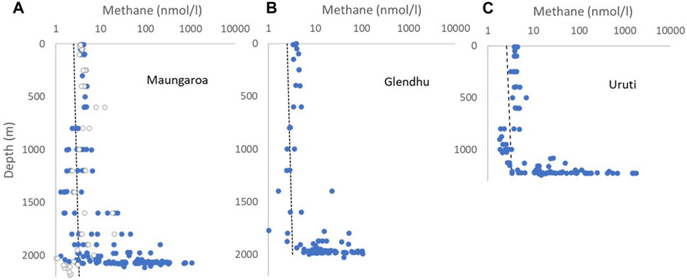
Figure 2. Vertical profiles of dissolved methane concentration (nmol/l) at the three seep sites: (A) Maungaroa, (B) Glendhu Ridge and (C) Uruti Ridge, with consistent depth and concentration scales used for comparison. The dashed line indicates the dissolved methane concentration expected from equilibrium with atmospheric methane. In (A) samples within 1 km of the Maungaroa seep are shown by blue circles, and those from background sites >1 km from the seep by open circles.

3.1.1 High resolution dissolved methane in bottom waters

Comparison of discrete sample and sensor data on three CTD tows at the Maungaroa seep (Figure 3) indicated that the sensor generally overestimated background dissolved methane concentration and underestimated high values. This was not surprising as diffusion limits the sensor response with equilibrium taking longer than exposure to the methane maximum during towing. This also resulted in a “memory” effect, with temporal smearing generating lower broad dissolved methane concentrations relative to the sharper and higher concentrations in the discrete bottle data (see Figure 3). Corrected in situ dissolved methane concentrations (CH_{4 insitu}) were generated from the sensor data by applying the equation CH_{4 insitu} = (CH4_sens −2)^1.15, which was derived from in situ calibration of the sensor relative to discrete bottom water samples. The limiting step of diffusion also caused a sensor response lag of ∼5–6 min, as confirmed by comparison of sensor and discrete sample data, and so the dissolved CH_{4 insitu} was also corrected for this delay (Figure 3). However, the in situ temporal lag was shorter than in pre-voyage laboratory tests, potentially reflecting increased diffusion at the elevated in situ pressure in bottom water. Although the sensor “memory” could not be explicitly determined, the combined concentration and temporal corrections showed good agreement between the calculated CH_{4 insitu} and the bottle data (Figures 3A, B), with some indication of smearing following the methane maxima.

Figure 3

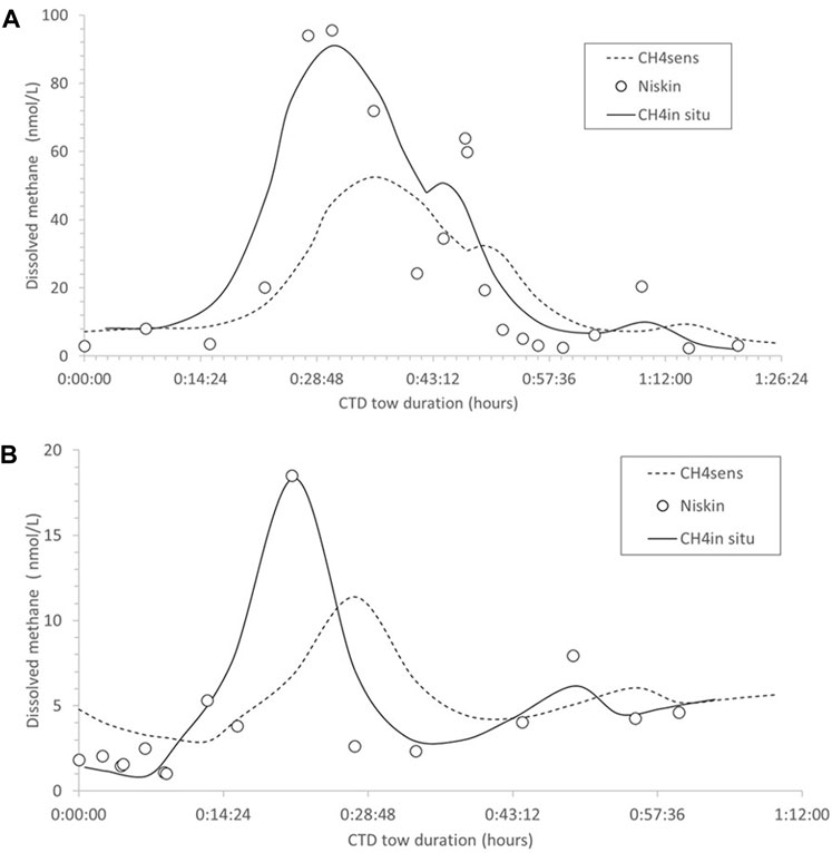
Figure 3. (A,B) CTD-sensor transects in bottom waters 5 m above the seafloor at Maungaroa, showing dissolved methane concentration (nmol/L) as determined by the sensor (CH_{4 sens}, dashed line), and discrete Niskin samples (open circles), overlain by the corrected sensor data (CH_{4 insitu}, black lines). The y-axis indicates the duration of the sensor tow in hours.

The lateral distribution of dissolved methane at Maungaroa was determined by a series of transects carried out with reference to the seep location and also elevated backscatter, which indicated the presence of authigenic carbonates formed by precipitation that is characteristic of seeps along the Hikurangi Margin (Figure 4C; Bowden et al., 2013; Crutchley et al., 2021). In two of the CTD transects dissolved methane associated with the bubble plume reached a water column depth of ∼1,600 m with lateral transport to the north-east (towards 4 in Figure 4B). Retention in bottom waters occurred, with over 50% of total dissolved methane within 50 m of the seafloor and 75% in the bottom 200 m. This largely reflects rapid diffusion of methane out of the bubbles (McGinnis et al., 2006), which is then transferred laterally in dissolved form by bottom currents. This may be supplemented by dissolved methane in fluid release at the seafloor (Krabbenhoeff et al., 2010), although these two sources are indistinguishable with the techniques employed in the current study.

Figure 4

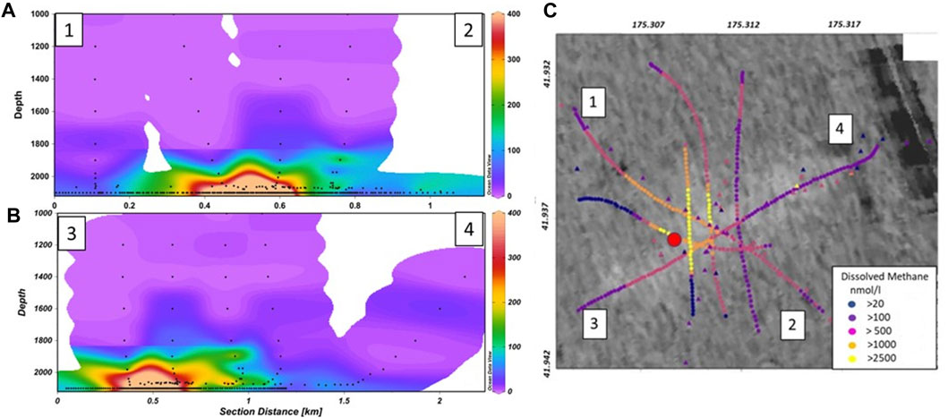
Figure 4. Contour plots showing the vertical distribution of dissolved methane concentration (nmol L⁻¹, see colour bar) below 1,000 m water depth along: (A) a NW–SE transect (1–2), and (B) a SW-NE transect (3–4) across the Maungaroa seep, with sample depths indicated by the black dots. (C) shows the spatial distribution of dissolved methane (nmol/l, see key), from discrete bottle samples (triangles) and sensor measurements (circles), overlain on subsurface backscatter around the Maungaroa seep, with transects 1–2 and 3–4 and mooring location (red dot) identified. The elevated backscatter in the upper right of (C) is an artefact related to swell or outer beam noise. (A,B) were created using Ocean Data View (Schlitzer, 2021), and the spatial plot (C) using ArcGIS.

3.2 Bottom water currents and properties

Regional circulation in the water column overlying the Maungaroa Seep is influenced by eddies and mixing between the northward-flowing Southland Current and the D'Urville Current which flows through the Cook Strait. This generates the Wairarapa Coastal Current (WCC), a relatively cool northward flow along the outer shelf and upper slope (Figure 5D), inshore of the southward-flowing East Cape Current (ECC, Chiswell, 2003). The observed salinity variation between 200 m and 400 m (Figure 5C) likely reflects variability in the relative contributions of the Southland Current, ECC and D’Urville Current between sampling profiles. Below this the Antarctic Intermediate Water (AAIW) is evident as a salinity minimum around 1,000 m depth, with salinity increasing to the seafloor in Pacific Deep Water (PDW).

Figure 5

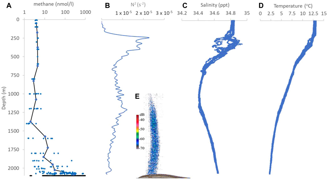
Figure 5. Water column profiles at Maungaroa showing: (A) methane concentration (nmol/l), from discrete samples (blue symbols), and corrected sensor data (CH_{4 insitu}, black points between 2070 and 2080 m depth), with bin average methane concentration (black line), (B) buoyancy frequency squared N² (20 m bin average), (C) salinity and (D) temperature at 1 m resolution from 12 separate vertical profiles. The inset (E) shows the bubble plume at the Maungaroa seep, as imaged by the 38 kHz channel in the multibeam data (reproduced with permission from Turco et al., 2022). All profiles and inset are scaled to the same vertical depth range.

The mean Buoyancy Frequency squared (N²) profile showed strongest vertical stratification between 250 m and 400 m depth at the base of the WCC (Figure 5B), and then decreased to the core of the AAIW at 1,000 m depth. N² subsequently increased to ∼1,250 m depth, at the interface between the AAIW and PDW, before decreasing again to the seafloor. Comparison with the dissolved methane profile at Maungaroa (Figure 5A; also Figures 4A, B) suggests that water column structure and stability have a limited influence on vertical dissolved methane distribution. The bubble plume extended to a water column depth of ∼1,000 m, shallower than the mid-water column stratification maximum at 1,250 m (compare Figures 5B, E), whereas dissolved methane was largely retained below 1,500 m where there was no corresponding N² maximum (compare Figures 5A, B). The absence of near-seafloor stratification (Figure 5B) is in contrast to Opouawe Bank nearby, where dissolved methane from a shallower seep (depth of ∼1,080 m) was constrained by elevated N² just above the seafloor (Law et al., 2010).

The mooring at Maungaroa was located less than 100 m from the seep centre, with sensor measurements at 15 m above the seafloor. The ADCP recorded relatively low currents (<0.15 m s⁻¹), with north-easterly flow dominating and tidal currents running along the shelf parallel to the coast (Supplementary Figure S1). Fitting of M2 tides confirmed that tidal forcing was the dominant factor, despite an apparent anomaly in flow direction on Day 2. The tidal influence was also apparent in bottom water temperature and salinity, which showed an inverse relationship and variability of <0.2°C and 0.02 ppt, respectively, over the 5-day period. Dissolved O₂ concentration showed minor variation of <2 μmol L^-1 relative to a bottom water mean of 152.5–155 μmol L^-1 (44.8%–45.5% saturation with respect to the atmosphere). This variability primarily reflected temperature-related variation in solubility and there was no temperature or dissolved O₂ signal associated with the seep plume (Supplementary Figure S1), as reported in a previous regional study (Krabbenhoefft et al., 2010).

3.3 Modelled near-field methane distribution

The modelled methane was scaled by reference to the observed dissolved methane concentration in bottom waters within a 1 km radius around the seep using the Gerris model to estimate the methane source function, which was then converted to a flux by applying this to a source volume. Figures 6A, B show two sensor tows that crossed the Maungaroa seep, with the modelled distribution at the corresponding tidal state shown in Figures 6C, D. Overlaying the transects in Figures 6C, D highlights the overriding influence of the tidal cycle on the spatial distribution of seep-derived methane in bottom waters; despite both transects passing within 50 m of the seep, the modelled methane concentrations and distribution differ markedly due to the tidal state, as shown in the corresponding model simulations.

Figure 6

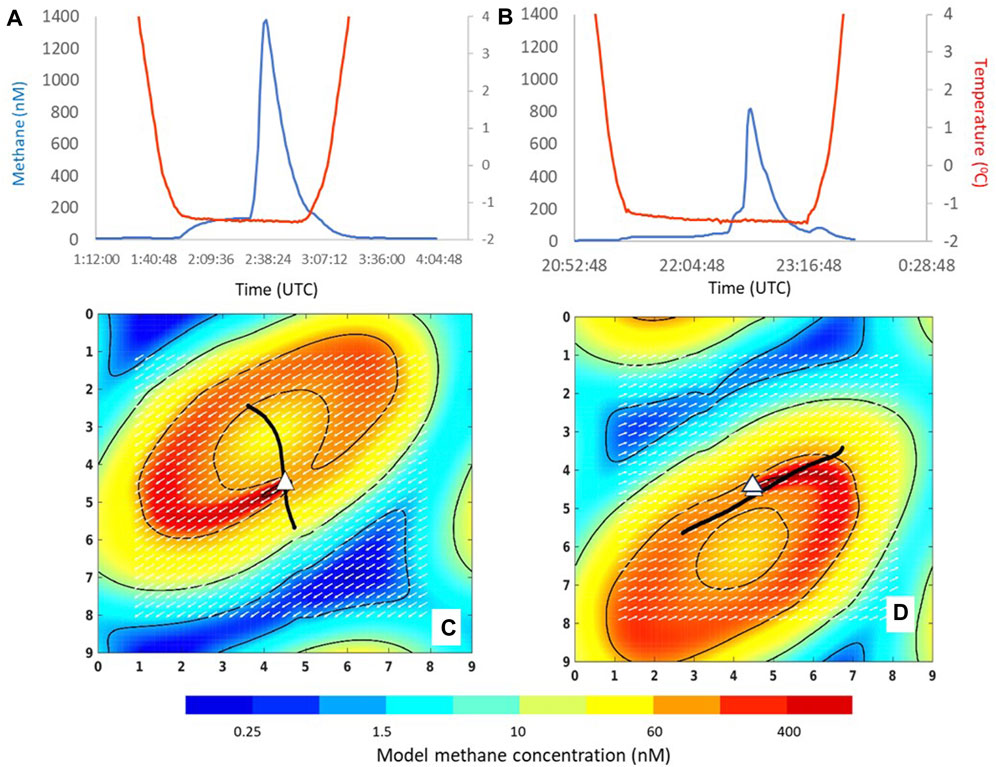
Figure 6. (A,B) Bottom water methane concentration (nM, blue line) and temperature (^oC, red line) during two sensor transects across the Maungaroa seep, shown against time (UTC) on the x-axis. (C,D) show the corresponding dissolved methane distribution in bottom water, based on data obtained in A and B, respectively, as generated by the Gerris model at 2.5 and 3.0 tidal cycles. The seep location is indicated by the white triangle, the sensor transects by the continuous black line, and the modelled dissolved methane concentration by colour corresponding to the underlying colour bar. The white arrows show the tidal flow vectors at the time of the concentration contour snapshot in each frame, to indicate how flow influences dispersal. The total domain is 2.25 km x 2.25 km, with the numbers on the x- and y-axis corresponding to increments of 250 m.

The footprint of the seep was assessed using different approaches. Previous measurement of water column backscatter indicated a seep footprint of ∼200 m² at Maungaroa (Crutchley et al., 2021), although this is likely an overestimate as the bubble plume will be dispersed over a broader area by bottom currents and advection relative to the actual seafloor release area. An alternative approach to estimating seep spatial extent utilized the decline in meiobenthos abundance from the seep centre to background (D. Leduc, pers. comm.) which provided a horizontal length scale of ∼50 m. As the latter estimate is consistent with the length scale reported for active fluid release at seeps along the Hikurangi Margin (Klaucke et al., 2010), a footprint of 50 m x 50 m was applied with the Gerris simulation, to generate a source function of 4.7 x 10⁻⁶ mol m⁻³ s⁻¹ methane, and so an annual methane emission of 3 x 10⁵ kg at the Maungaroa seep.

3.3.1 Modelled far-field dispersion of dissolved methane

ROMS-simulated bottom water currents were comparable with the ADCP currents in strength (<0.15 m s⁻¹) and direction, with north-easterly and south-easterly flow combining with tides to generate a net north-easterly advection (Figure 7A). Dye tracer released at the Maungaroa seep site in the ROMS simulation advected along the 2000 m isobath a maximum distance of ∼87 km north-east of the seep location over 1 year. Scaling the ROMS tracer concentration to the Gerris-derived source function showed that modelled methane concentration was highest in a plume extending north-east of the seep centre (Figure 7B), but this declined sharply, falling below 500 and 200 nmol L⁻¹ within 10 and 20 km of the seep location, respectively, with a total plume surface area of 4,000 km² after 1 year (see Supplementary Table S2).

Figure 7

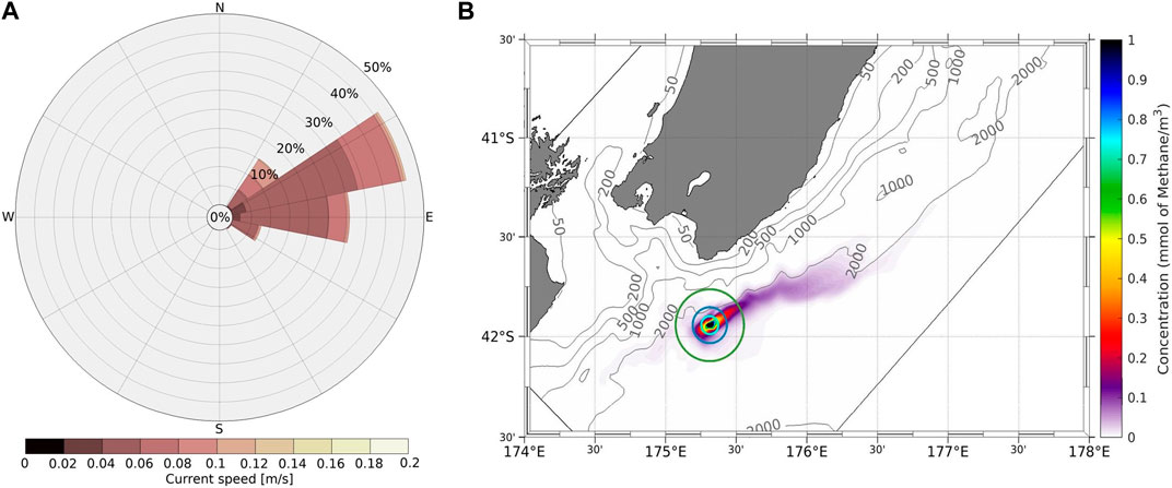
Figure 7. (A) Rose of current speed (m/s) averaged over a polygon spanning the methane seep locations. (B) Time-averaged dissolved methane concentration (mmol m⁻³) for Maungaroa for the simulation period 1 January 2013–16 December 2013, with the turquoise, blue and green concentric circles indicating radii of 5 km, 10 km and 20 km from the release point, respectively. The modelled dissolved methane concentration is shown on the colour bar, with isobaths indicated by the grey contours.

The ROMS model was subsequently applied across the south-east Hikurangi Margin to assess plume dispersion for the four other cold seeps, characterized by Turco et al. (2022); see Table 1). Although the tracer was advected primarily to the north-east at Maungaroa (Figures 7, 8), individual snapshots of tracer concentration over the simulation period showed that some seep plumes advected south-west on occasions (Figure 9). Lateral plume dispersion varied between seeps, with the tracer released at Pahaua Bank advecting a maximum distance of 104 km between the 1,000 m and 2000 m isobaths, in contrast to the shallower Uruti Ridge site, where dispersal was only 50 km within a year. At all sites elevated dye concentration (>0.25%) was generally constrained within 10 km of the release location, although elevated tracer plumes occasionally extended 50 km from the release site (Figure 9).

Figure 8

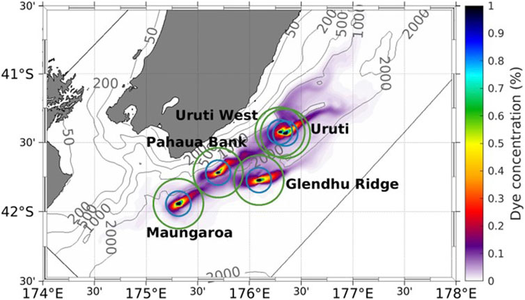
Figure 8. Time-averaged concentration of dye tracer at the five seep locations on the south-east Hikurangi Margin for the period 1 January 2013–16 December 2013. The blue and green circles show radii of 10 and 20 km, respectively, from the release point at each seep. Dye tracer is shown as a percentage relative to 1.0 at the source location, as indicated in the colour bar, with isobaths indicated by the grey contours.

Figure 9

Figure 9. (A–D) Daily snapshots of dye tracer concentration on the south-east Hikurangi Margin at four different timepoints between 1 January 2013 and 16 December 2013. The blue and green circles indicate radii of 10 and 20 km, respectively, from the release point at each location. Dye tracer is shown as a percentage relative to 1.0 at the source location, as indicated in the colour bar, with isobaths indicated by the grey contours.

The extent of the dye tracer footprint for each seep plume was estimated based on a polygon enclosed by the contour associated with a dye concentration of 0.005. After 1 year the surface area of the individual dye tracer plumes ranged from 2,370 to 4,000 km² (Supplementary Table S2). The modelled vertical plume dispersal extended 1,000 m above the seafloor, resulting in a combined plume volume for the five seeps of 3,500 km³ (Supplementary Table S3). The combination of reversing tidal currents, the relative proximity of seeps and their co-location primarily at similar depths resulted in overlap of the tracer plumes from individual seeps. This is evident as extended plumes of elevated tracer concentration (>0.25%) beyond 20 km from the seep location on occasions, such as for Maungaroa and Glendhu Ridge in September 2013 (Figure 9C). The ratio of the Gerris model flux estimate to the hydroacoustic flux estimate for Maungaroa (Turco et al., 2022) was then applied to the other seeps in Table 1 to generate a total methane flux for the five seeps of 0.4–3.2 x 10⁶ kg CH₄ y^-1. Extrapolating this estimate using the approach of Turco et al. (2022) to all seeps across the Hikurangi Margin (Watson et al., 2020) results in a total methane emission of 1.1–10.9 x 10⁷ kg CH₄ y^-1.

3.4 Potential methane oxidation rate

Measurements in 15 bottom water samples obtained within 1 km of the three seep sites (Maungaroa, Uruti Ridge and Glendhu Ridge) generated potential methane oxidation rates of 1.79 ± 0.64 nM d⁻¹ (Supplementary Figure S2). Rates were relatively insensitive to bottom water DIC concentration (mean 2058.1 $\mu$ mol kg^-1), and also showed no trend with distance from seep location or between the three seeps. In addition, there was no relationship between potential oxidation rate and in situ methane concentration, despite three orders of magnitude variation in the latter (Supplementary Figure S2).

3.5 Dissolved δ¹³C-CH₄

Hydrates release methane with a characteristic low stable isotope (δ¹³C-CH₄) value that results from fractionation during bacterial methanogenesis (Reeburgh, 2007), and consequently elevated methane concentrations in bottom water overlying the Hikurangi Margin seeps were associated with low δ¹³C-CH₄. The three seep sites showed a similar relationship between dissolved methane concentration and δ¹³C-CH₄ in waters between 1,000 m depth and the seafloor (Figure 10A), suggesting that there was no significant differences in either the source or processing of methane in bottom waters at the three sites. However, the more extensive dataset obtained at Maungaroa showed greater variability than the other two sites. Analysis of data from this site for the bottom 200 m of water, where most seep methane was retained (Figures 4, 5), showed a linear relationship between methane concentration and δ¹³C-CH₄ (Figure 10B), as would be expected for lateral mixing of seep-derived methane with background water. However, variability precluded identification of end-member values, and indicated the influence of other factors.

Figure 10

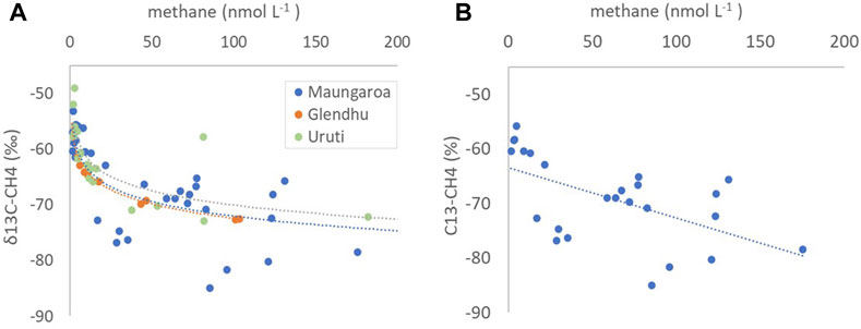
Figure 10. (A) The relationship between dissolved methane concentration (nmol L⁻¹) and δ¹³C-CH₄ values (‰) at depths >1,000 m for the three main seep sites, with the fits indicated by dotted lines and corresponding color for each seep (see key) (B) Dissolved methane concentration - δ¹³C-CH₄ relationship for Maungaroa in bottom water up to 200 m above the seafloor, with the dashed line indicating the mean linear fit.

4 Discussion

4.1 Methane emissions

Integration of in situ measurements in the Gerris model and ROMS simulation provided a new approach to estimating methane seep emissions on the Hikurangi Margin. The resulting methane flux for the Maungaroa seep of 3 x 10⁵ kg CH₄ y^-1 is 4%–12% of a previous estimate of 2.5–7.2 × 10⁶ kg CH₄ y^-1 derived from hydroacoustic data (Turco et al., 2022). These different estimates reflect methodological assumptions and uncertainties, as described in Turco et al. (2022) and other studies (Mitchell, et al., 2022). The hydroacoustic calculation likely overestimates the flux, as diffusive loss of methane during bubble rise (McGinnis et al., 2006) was not accounted for, whereas the Gerris model included uncertainty regarding the spatial dimensions of the methane source (see Section 3.3). The dissolved methane measurements in this study may also have included fluid input, although previous regional studies indicate that fluid release is relatively minor in relation to free gas (Luo et al., 2016). Although emissions from seeps are generally consistent in terms of location and magnitude on the Hikurangi Margin (Law et al., 2010), temporal variation in emissions has been reported (Naudts et al., 2010). Consequently, the emission estimates in this study and that of Turco et al. (2022) provide boundaries on annual methane emissions at Maungaroa of 0.3–7.2 x 10⁶ kg CH₄ y^-1. This estimate is high relative to other seeps on Hikurangi Margin, for which annual emissions range from 10² to 10⁴ kg CH₄ y^-1 (Naudts et al., 2010; Luo et al., 2016), but is consistent with a first order estimate derived from hydroacoustic data and residence time for the Opouawe Bank seep located at a shallower depth close to Maungaroa (4.9–9.8 x 10⁵ kg CH₄ y^-1, Law et al., 2010). The revised methane emission for the entire Hikurangi Margin, of 1.1–10.9 x 10⁷ kg CH₄ y^-1, is equivalent to 0.8%–7.9% of New Zealand terrestrial emissions (Ministry for Environment, 2022), and of similar magnitude to the calculated air-sea methane flux for the entire New Zealand Exclusive Economic Zone (4.1 x 10⁷ kg y⁻¹, based upon 130% surface supersaturation; Law et al., 2010). This highlights the critical role of horizontal dilution and the pelagic methane filter in minimizing transfer of seep-derived methane to the atmosphere.

4.2 The relative roles of methane oxidation and dispersion

A primary aim of this study was to distinguish the relative contributions of dilution and methanotrophy in determining the distribution and concentration of methane in bottom waters along the Hikurangi Margin. The observed decrease in methane concentration in the vicinity of the seep, and corresponding diffusion and advection in the Gerris model, indicate dilution of two orders of magnitude. The equivalent dilution rate of ∼1 mol m^-3 d⁻¹ is considerably larger than the measured potential oxidation rate of ∼2 x 10⁻⁶ mol m⁻³ d⁻¹ and, consequently, advection and dilution are the dominant determinants of methane concentration for the volume of interest and timescales of days in this study.

However, methanotrophy is an important sink for dissolved methane that not only reduces methane concentrations in the deep ocean but also flux to the atmosphere (Mao et al., 2022). The potential contribution of methanotrophy in this study was examined by two independent techniques: measurement of potential oxidation rate in isotope tracer incubations and interpretation of the dissolved δ¹³C-CH₄ values in bottom waters. The potential oxidation rates were relatively invariant, despite being sampled from within the seep plume through to background locations at all three seep sites (Supplementary Figure S2). This uniformity could reflect tidal retention in bottom waters along the shelf (Figure 9), resulting in a homogenised methanotroph community with uniform oxidation capacity. Although the potential oxidation rate technique relies upon addition of isotopic tracer at concentrations in excess of in situ methane concentrations (Leonte et al., 2018), the observed range and low variability are similar to rates reported at other seeps (5.6 ± 2.3 nM d⁻¹; Leonte et al., 2017; 0–3 nM d⁻¹; Graves et al., 2015; 0–2.5 nM d⁻¹; Weinstein et al., 2016), and marine systems (0–2.5 nM d⁻¹, Steinle et al., 2015; Osudar et al., 2015; 1–10 nM d⁻¹; Mau et al., 2013; 0.01–7.5 nM d⁻¹; Mao et al., 2022). This consistency is surprising, considering the range of environments and ambient methane concentrations, and also the different techniques used to measure methane oxidation. However, it should be noted that rate measurements in this and other studies were predominately carried out at atmospheric pressure, which may alter microbial metabolism and so methane oxidation, relative to that at in situ pressure in the deep ocean (Fortunato et al., 2021).

The absence of a relationship between potential oxidation rate and in situ methane concentration, despite three orders of magnitude variation in the latter (Supplementary Figure S2), has been reported in other studies. However, a first-order relationship has also been reported for some hydrate seeps (Valentine et al., 2001), and hydrothermal plumes (de Angelis et al., 1993), with strong evidence from the Deep Water Horizon wellhead blowout in the Gulf of Mexico after which rates rose by four orders of magnitude (Crespo-Medina et al., 2014). Methanotrophic response is slow (Valentine et al., 2001), with rates increasing ∼1–2 months after methane addition and reaching a maximum after 3–4 months, as confirmed by modelling, oxidation rate and in situ O₂ measurements in the Gulf of Mexico (Kessler et al., 2011; Du and Kessler, 2012; Crespo-Medina et al., 2014). This may reflect slow adjustment of methanotroph metabolism or alternatively adaptation at the community level to elevated methane, which may account for the absence of a relationship between oxidation rate and in situ dissolved methane concentration (Supplementary Figure S2). Alternatively, this lag may reflect other controls of methane oxidation (Steinle et al., 2016), as suggested by shorter response times to methane addition at near-seep sites relative to sites at distance (Chan et al., 2019). As dilution was excluded in the Chan et al. study, the results suggest that near-seep methanotrophs were primed by prior exposure to elevated methane, or alternatively availability of a limiting factor such as trace metals or macronutrients (De Angelis et al., 1993; Beal et al., 2009).

The relatively constant potential oxidation rate across three orders of magnitude in dissolved methane concentration in this study resulted in a range in turnover time of 6–1,000 days, consistent with other systems (7–560 days, De Angelis et al., 1993; 3–1,000 days; Osudar et al., 2015; 500 days to decades; Valentine et al., 2001). However, shorter turnover times have been recorded at seeps where mixing and circulation is constrained (0.3–3.7 days, Leonte et al., 2017; 1.3–24.0 days; Weinstein et al., 2016). Indeed, residence time is an important determinant of methane oxidation rate, with regional geomorphology, seasonal and water mass variation influencing methanotroph distribution, abundance and activity via dilution and current flow (Steinle et al., 2016; Gründger et al., 2021). The Maungaroa seep is located on a relatively flat ridge on the Hikurangi Margin (Turco et al., 2022), without canyons or seafloor morphology that might enhance regional retention and entrainment of bottom water, and so accumulation of dissolved methane, and thus methane oxidation, might be expected to be low. Although this is supported by the linear relationship between methane concentration and δ¹³C-CH₄ in bottom waters, other influences are also apparent (Figure 10B). This may reflect tidal circulation and entrainment of methane in the vicinity of the seep, as visualized in the Gerris and ROMS model simulations (Figures 6 and 9), with fresh seep methane of lower δ¹³C-CH₄ mixing with recirculated “older” methane with higher δ¹³C-CH₄ values due to oxidation. Despite potential methane oxidation rates being low (Supplementary Figure S2) relative to mixing, local retention could enhance methanotroph adaptation to elevated methane, resulting in higher δ¹³C-CH₄ values. Conversely, the variability at Maungaroa in Figure 10B may arise due to methane input from other regional seeps, as illustrated in the ROMS simulation in Figure 9. Methane release from hydrates will not have a uniform regional isotopic value but will vary between sites. In addition, thermogenic methane input has been reported for the Hikurangi Margin (Henrys et al., 2009), which could be a source of methane with higher δ¹³C-CH₄. Although tidal circulation of bottom waters may increase methane oxidation and mixing with methane from other sources this also confounds determination of their relative contribution to local methane dynamics.

4.3 Potential influence of methane emissions on water column biogeochemistry

Methane oxidation provides a source of energy and C for methanotroph growth (Hanson and Hanson, 1996), and ultimately produces CO₂ whilst consuming O₂. This is reflected in the elevated O₂ consumption in seafloor seep communities relative to non-seep benthos (Boetius and Wenzhöfer, 2013), that arises directly from methanotrophy and indirectly from chemosynthetically-supported benthic communities. However, there was no evidence of the Hikurangi Margin seeps influencing bottom water O₂ concentrations in either the mooring data (Supplementary Figure S1) or CTD profiles (data not shown), and the measured potential methane oxidation rates would have negligible effect on bottom water O₂. If the total methane release by the five seeps was completely oxidized within the modeled plume volume (90% of dye tracer, ∼1,000 km³) within 1 year, the decrease in dissolved O₂ concentration would be <0.3%. This assumes utilization of 2 mol of O₂ during methanotrophy and so conversion of all methane-fueled biomass to CO₂ (Chan et al., 2019), with resulting CO₂ production of <0.2 μmol L^-1 and a corresponding decrease in pH of <0.002 relative to a background of 7.87. This minor influence is consistent with observations at the Hudson Canyon seeps, where aerobic methane oxidation accounted for only 0.3% of observed changes in DIC (Garcia-Tigreros and Kessler, 2018). A previous estimate based upon all Hikurangi Margin seeps suggested a greater impact of methane oxidation on dissolved O₂ and the carbonate system (Turco et al., 2022), but this was derived using a higher seep methane flux and also did not consider dilution and dispersion. Although the current assessment indicates negligible impact of seep methane on bottom water biogeochemistry it does not account for superimposition of plumes from different seeps along the Hikurangi Margin, as shown in Figure 9, which may result in localized impacts. For example, oxidation of seep methane in overlapping plumes could generate localized decreases of 0.53% in dissolved O₂ concentration and 0.005 in pH. These localized methanotrophy-driven decreases would compound the current low dissolved O₂ saturation in deep water along the Hikurangi Margin, and contribute to ongoing deoxygenation and carbonate saturation horizon shoaling (Feely et al., 2012; Oschlies et al., 2018).

4.4 Characterizing seep dispersal using hydrodynamic models

This study highlights the value of assessing the influence of methane seeps on bottom waters by integrating observations within a hydrodynamic framework. Although bottom water currents confound characterization of dissolved methane distribution around a seep, as illustrated in Figure 6, tidal dispersion and dilution was accounted for in a Gerris model. The ROMS model subsequently simulated methane concentration and distribution using the source function and location generated by the Gerris model but did not include loss to methane oxidation. Although rate measurements indicate that this process is insignificant relative to dispersion, further model development should incorporate methane oxidation, informed by measurements along the Hikurangi Margin to investigate the apparent uniformity in rate and also establish the relative contribution of oxidation to bottom water methane dynamics. The superimposition of multiple seeps could be further examined by applying the ROMS framework to the full suite of seeps along the Hikurangi Margin (Watson et al., 2020). As with many global studies, methane release from seeps is not apparent in surface waters along the Hikurangi Margin, except for some shallow seeps (Higgs et al., 2019); however, there is the potential for transfer via vertical mixing associated with geomorphological features and eddies. Application of the ROMS model framework to the broader shelf region could determine whether this represents a “shortcut” for seep methane transfer to surface waters and flux to the atmosphere along the Hikurangi Margin. The ROMS simulation also suggests that tidal retention and superimposition of plumes may facilitate connectivity between seeps, which should be examined with respect to larval dispersion and connectivity between seep populations (Levin et al., 2016) along the broader Hikurangi Margin. In addition, integration of regional hydrodynamic models with Earth System Models (Rickard et al., 2023) could examine future climate-driven changes in bottom water and the associated biogeochemical impacts along the Hikurangi Margin.

5 Conclusion

Integration of methane data in a ROMS simulation established the methane source strength of five cold seeps on the south-eastern slope of the Hikurangi Margin. Although the combined methane plumes dispersed over a volume of 3,500 km³ and depth of 1,000 m over a year, elevated concentrations were largely restricted to bottom waters 20 km downstream of the seep location. Potential methane oxidation rates were low and invariant in bottom waters, regardless of dissolved methane concentration, indicating slow turnover of dissolved methane. Despite dilution being orders of magnitude greater than aerobic oxidation, δ¹³C-CH₄ values showed some variability in bottom waters, reflecting a potential contribution of methane oxidation or other sources. The total methane release was revised to 0.4–3.2 x 10⁶ kg CH₄ y^-1 for the five seeps, and 1.1–10.9 x 10⁷ kg CH₄ y^-1 for the entire Hikurangi Margin, equivalent to the estimated air-sea flux for the entire Exclusive Economic Zone but less than 8% of New Zealand terrestrial emissions. Oxidation of total annual emissions from the five seeps would not significantly affect bottom water O₂, CO₂ and pH; however, superimposition of plumes from different seeps could support localised maxima in methane and methanotrophy in bottom waters. Integration of methane concentration within a hydrodynamic framework provides insight into the relative roles of dilution and oxidation in determining dissolved methane concentration in bottom waters, and also an approach for assessing the contribution to and sensitivity of cold seeps to climate change.

Data availability statement

The datasets presented in this study can be found in online repositories. The names of the repository/repositories and accession number(s) can be found below: Data and animations of the seep dispersal are available at https://zenodo.org/records/10373095.

Author contributions

CL: Conceptualization, Data curation, Formal Analysis, Funding acquisition, Investigation, Methodology, Project administration, Resources, Writing–original draft, Writing–review and editing. CC: Data curation, Investigation, Methodology, Software, Visualization, Writing–review and editing. AM: Data curation, Investigation, Methodology, Resources, Writing–review and editing. SB: Methodology, Resources, Writing–review and editing. JB: Formal Analysis, Investigation, Methodology, Resources, Writing–review and editing. GR: Data curation, Formal Analysis, Investigation, Methodology, Software, Validation, Visualization, Writing–review and editing.

Funding

The author(s) declare that financial support was received for the research, authorship, and/or publication of this article. Funding for this work was provided by the New Zealand Hīkina Whakatutuki MBIE Endeavor Fund Programme Gas Hydrates: Economic Opportunities and Environmental Impact (HYDEE; contract CO5X1708), with support from Strategic Scientific Investment Funds to the NIWA Ocean Centre.

Acknowledgments

We thank the Officers and Crew of the R/V Tangaroa, Ashley Rowden for voyage leadership; Brett Grant, Fiona Elliot and Chris Ray for mooring design and construction; Sarah Searson for mooring deployment and recovery; Josette Delgado for stable isotope analysis; Kim Currie and Judith Murdoch for carbonate system analysis; Steve George and Sarah Searson for CTD operations; Dave Bowden for DTIS location data; Susi Woelz for the site map, Arne Pallentin for ArcGIS data manipulation, and Sarah Seabrook for constructive comments.

Conflict of interest

The authors declare that the research was conducted in the absence of any commercial or financial relationships that could be construed as a potential conflict of interest.

Publisher’s note

All claims expressed in this article are solely those of the authors and do not necessarily represent those of their affiliated organizations, or those of the publisher, the editors and the reviewers. Any product that may be evaluated in this article, or claim that may be made by its manufacturer, is not guaranteed or endorsed by the publisher.

Supplementary material

The Supplementary Material for this article can be found online at: https://www.frontiersin.org/articles/10.3389/feart.2024.1354388/full#supplementary-material

References

Assayag, N., Rivé, K., Ader, M., Jézéquel, D., and Agrinier, P. (2006). Improved method for isotopic and quantitative analysis of dissolved inorganic carbon in natural water samples. Rapid Commun. Mass Spectrom. 20, 2243–2251. doi:10.1002/rcm.2585

PubMed Abstract | CrossRef Full Text | Google Scholar

Barnes, P. M., Lamarche, G., Bialas, J., Henrys, S., Pecher, I., Netzeband, G. L., et al. (2010). Tectonic and geological framework for gas hydrates and cold seeps on the Hikurangi subduction margin, New Zealand. Mar. Geol. 272 (1-4), 26–48. doi:10.1016/j.margeo.2009.03.012

CrossRef Full Text | Google Scholar

Beal, E. J., House, C. H., and Orphan, V. J. (2009). Manganese-and iron-dependent marine methane oxidation. Science 325 (5937), 184–187. doi:10.1126/science.1169984

PubMed Abstract | CrossRef Full Text | Google Scholar

Biastoch, A., Treude, T., Rüpke, L. H., Riebesell, U., Roth, C., Burwicz, E. B., et al. (2011). Rising Arctic Ocean temperatures cause gas hydrate destabilization and ocean acidification. Geophys. Res. Lett. 38 (8). doi:10.1029/2011gl047222

CrossRef Full Text | Google Scholar

Boetius, A., and Wenzhöfer, F. (2013). Seafloor oxygen consumption fuelled by methane from cold seeps. Nat. Geosci. 6 (9), 725–734. doi:10.1038/ngeo1926

CrossRef Full Text | Google Scholar

Boudreau, B. P., Luo, Y., Meysman, F. J., Middelburg, J. J., and Dickens, G. R. (2015). Gas hydrate dissociation prolongs acidification of the Anthropocene oceans. Geophys. Res. Lett. 42 (21), 9337–9344. doi:10.1002/2015gl065779

CrossRef Full Text | Google Scholar

Bowden, D. A., Rowden, A. A., Thurber, A. R., Baco, A. R., Levin, L. A., and Smith, C. R. (2013). Cold seep epifaunal communities on the Hikurangi margin, New Zealand: composition, succession, and vulnerability to human activities. PLoS ONE 8 (10), e76869. doi:10.1371/journal.pone.0076869

PubMed Abstract | CrossRef Full Text | Google Scholar

Chan, E. W., Shiller, A. M., Joung, D. J., Arrington, E. C., Valentine, D. L., Redmond, M. C., et al. (2019). Investigations of aerobic methane oxidation in two marine seep environments: Part 1—chemical kinetics. J. Geophys. Res. Oceans 124 (12), 8852–8868. doi:10.1029/2019jc015594

CrossRef Full Text | Google Scholar

Chassignet, E. P., Hurlburt, H. E., Metzger, E. J., Smedstad, O. M., Cummings, J. A., Halliwell, G. R., et al. (2009). US GODAE: global ocean prediction with the Hybrid Coordinate Ocean Model (HYCOM). Oceanography 22 (2), 64–75. doi:10.5670/oceanog.2009.39

CrossRef Full Text | Google Scholar

Chiswell, S. M. (2003). Circulation within the Wairarapa eddy, New Zealand. N. Z. J. Mar. Freshw. Res. 37 (4), 691–704. doi:10.1080/00288330.2003.9517199

CrossRef Full Text | Google Scholar

Crespo-Medina, M., Meile, C. D., Hunter, K. S., Diercks, A. R., Asper, V. L., Orphan, V. J., et al. (2014). The rise and fall of methanotrophy following a deepwater oil-well blowout. Nat. Geosci. 7 (6), 423–427. doi:10.1038/ngeo2156

CrossRef Full Text | Google Scholar

Crutchley, G. J., Hillman, J. I., Kroeger, K. F., Watson, S. J., Turco, F., Mountjoy, J. J., et al. (2023). Both longitudinal and transverse extension controlling gas migration through submarine anticlinal ridges, New Zealand's southern Hikurangi margin. J. Geophys. Res. Solid Earth 128 (6), e2022JB026279. doi:10.1029/2022jb026279

CrossRef Full Text | Google Scholar

Crutchley, G. J., Mountjoy, J. J., Hillman, J. I. T., Turco, F., Watson, S., Flemings, P. B., et al. (2021). Upward doming zones of gas hydrate and free gas at the bases of gas chimneys, New Zealand's Hikurangi margin. J. Geophys. Res. Solid Earth 126, e2020JB021489. doi:10.1029/2020jb021489

CrossRef Full Text | Google Scholar

De Angelis, M. A., Lilley, M. D., and Baross, J. A. (1993). Methane oxidation in deep-sea hydrothermal plumes of the endeavour segment of the juan de Fuca ridge. Deep Sea Res. Part I Oceanogr. Res. Pap. 40 (6), 1169–1186. doi:10.1016/0967-0637(93)90132-m

CrossRef Full Text | Google Scholar

Dickson, A., and Millero, F. (1987). A comparison of the equilibrium constants for the dissociation of carbonic acid in seawater media. Deep Sea Res. 34, 1733–1743. doi:10.1016/0198-0149(87)90021-5

CrossRef Full Text | Google Scholar

Dickson, A., Sabine, C., and Christian, J. (2007). “Guide to best Practices for ocean CO₂measurements,” in PICES special publication 3 IOCCP report (Sidney, BC: North Pacific Marine Science Organization).

Google Scholar

Du, M., and Kessler, J. D. (2012). Assessment of the spatial and temporal variability of bulk hydrocarbon respiration following the Deepwater Horizon oil spill. Environ. Sci. Technol. 46 (19), 10499–10507. doi:10.1021/es301363k

PubMed Abstract | CrossRef Full Text | Google Scholar

Faure, K., Greinert, J., von Deimling, J. S., McGinnis, D. F., Kipfer, R., and Linke, P. (2010). Methane seepage along the Hikurangi Margin of New Zealand: geochemical and physical data from the water column, sea surface and atmosphere. Mar. Geol. 272 (1-4), 170–188. doi:10.1016/j.margeo.2010.01.001

CrossRef Full Text | Google Scholar

Feely, R. A., Sabine, C. L., Byrne, R. H., Millero, F. J., Dickson, A. G., Wanninkhof, R., et al. (2012). Decadal changes in the aragonite and calcite saturation state of the Pacific Ocean. Glob. Biogeochem. Cycles 26 (3), 4157. doi:10.1029/2011gb004157

CrossRef Full Text | Google Scholar

Fortunato, C. S., Butterfield, D. A., Larson, B., Lawrence-Slavas, N., Algar, C. K., Zeigler Allen, L., et al. (2021). Seafloor incubation experiment with deep-sea hydrothermal vent fluid reveals effect of pressure and lag time on autotrophic microbial communities. Appl. Environ. Microbiol. 87 (9), 000788–e121. doi:10.1128/aem.00078-21

CrossRef Full Text | Google Scholar

Garcia-Tigreros, F., and Kessler, J. D. (2018). Limited acute influence of aerobic methane oxidation on ocean carbon dioxide and pH in Hudson canyon, northern U.S. Atlantic margin. J. Geophys. Res. Biogeosciences 123, 2135–2144. doi:10.1029/2018jg004384

CrossRef Full Text | Google Scholar

Graves, C. A., Steinle, L., Rehder, G., Niemann, H., Connelly, D. P., Lowry, D., et al. (2015). Fluxes and fate of dissolved methane released at the seafloor at the landward limit of the gas hydrate stability zone offshore western Svalbard. J. Geophys. Res. Oceans 120, 6185–6201. doi:10.1002/2015jc011084

CrossRef Full Text | Google Scholar

Gründger, F., Probandt, D., Knittel, K., Carrier, V., Kalenitchenko, D., Silyakova, A., et al. (2021). Seasonal shifts of microbial methane oxidation in Arctic shelf waters above gas seeps. Limnol. Oceanogr. 66 (5), 1896–1914. doi:10.1002/lno.11731

CrossRef Full Text | Google Scholar

Haidvogel, D. B., Arango, H., Budgell, W. P., Cornuelle, B. D., Curchitser, E., Di Lorenzo, E., et al. (2008). Ocean forecasting in terrain-following coordinates: formulation and skill assessment of the regional Ocean modeling system. J. Comput. Phys. 227, 3595–3624. doi:10.1016/j.jcp.2007.06.016

CrossRef Full Text | Google Scholar

Hanson, R. S., and Hanson, T. E. (1996). Methanotrophic bacteria. Microbiol. Rev. 60, 439–471. doi:10.1128/mr.60.2.439-471.1996

PubMed Abstract | CrossRef Full Text | Google Scholar

Henrys, S. A., Ellis, S., and Uruski, C. (2003). Conductive heat flow variations from bottom-simulating reflectors on the Hikurangi margin, New Zealand. Geophys. Res. Lett. 30 (2). doi:10.1029/2002gl015772

CrossRef Full Text | Google Scholar

Henrys, S. A., Woodward, D. J., and Pecher, I. A. (2009). “Variation of bottom-simulating-reflection strength in a high-flux methane province, Hikurangi margin, New Zealand,” in Natural gas hydrates - energy resource potential and associated geologic hazards. Editors T. Collett, A. Johnson, C. Knapp, and R. Boswell (AAPG Memoir), 481–489.

Google Scholar

Hester, K. C., and Brewer, P. G. (2009). Clathrate hydrates in nature. Annu. Rev. Mar. Sci. 1, 303–327. doi:10.1146/annurev.marine.010908.163824

PubMed Abstract | CrossRef Full Text | Google Scholar

Higgs, B., Mountjoy, J. J., Crutchley, G. J., Townend, J., Ladroit, Y., Greinert, J., et al. (2019). Seep-bubble characteristics and gas flow rates from a shallow-water, high-density seep field on the shelf-to-slope transition of the Hikurangi subduction margin. Mar. Geol. 417, 105985. doi:10.1016/j.margeo.2019.105985

CrossRef Full Text | Google Scholar

Kalnay, E., Kanimitsu, M., Kistler, R., Collins, W., Deaven, D., Gandin, L., et al. (1996). The NCEP/NCAR 40-year reanalysis Project. Bull. Am. Meteorological Soc. 77 (3), 437–471. doi:10.1175/1520-0477(1996)077<0437:tnyrp>2.0.co;2

CrossRef Full Text | Google Scholar

Karl, D. M., Beversdorf, L., Björkman, K. M., Church, M. J., Martinez, A., and Delong, E. F. (2008). Aerobic production of methane in the sea. Nat. Geosci. 1 (7), 473–478. doi:10.1038/ngeo234

CrossRef Full Text | Google Scholar

Kessler, J. D., Valentine, D. L., Redmond, M. C., Du, M., Chan, E. W., Mendes, S. D., et al. (2011). A persistent oxygen anomaly reveals the fate of spilled methane in the deep Gulf of Mexico. Science 331 (6015), 312–315. doi:10.1126/science.1199697

PubMed Abstract | CrossRef Full Text | Google Scholar

Klaucke, I., Weinrebe, W., Petersen, C. J., and Bowden, D. (2010). Temporal variability of gas seeps offshore New Zealand: multi-frequency geoacoustic imaging of the Wairarapa area, Hikurangi margin. Mar. Geol. 272 (1-4), 49–58. doi:10.1016/j.margeo.2009.02.009

CrossRef Full Text | Google Scholar

Klauda, J. B., and Sandler, S. I. (2005). Global distribution of methane hydrate in ocean sediment. Energy Fuels. 19, 459–470. doi:10.1021/ef049798o

CrossRef Full Text | Google Scholar

Krabbenhöft, A., Netzeband, G. L., Bialas, J., and Papenberg, C. (2010). Episodic methane concentrations at seep sites on the upper slope Opouawe Bank, southern Hikurangi Margin, New Zealand. Mar. Geol. 272 (1-4), 71–78. doi:10.1016/j.margeo.2009.08.001

CrossRef Full Text | Google Scholar

Lane, E. M., Walters, R. A., Gillibrand, P., and Uddstrom, M. (2009). Operational forecasting of sea level height using an unstructured grid ocean model. Ocean. Model. 28, 88–96. doi:10.1016/j.ocemod.2008.11.004

CrossRef Full Text | Google Scholar

Law, C. S., Nodder, S. D., Mountjoy, J., Marriner, A., Orpin, A., Pilditch, C. A., et al. (2010). Geological, hydrodynamic and biogeochemical variability of a New Zealand deep-water methane cold seep during an integrated three year time-series study. Mar. Geol. 272, 189–208. doi:10.1016/j.margeo.2009.06.018

CrossRef Full Text | Google Scholar

Leonte, M., Kessler, J. D., Kellermann, M. Y., Arrington, E. C., Valentine, D. L., and Sylva, S. P. (2017). Rapid rates of aerobic methane oxidation at the feather edge of gas hydrate stability in the waters of Hudson Canyon, US Atlantic Margin. Geochimica Cosmochimica Acta 204, 375–387. doi:10.1016/j.gca.2017.01.009

CrossRef Full Text | Google Scholar

Leonte, M., Wang, B., Socolofsky, S. A., Mau, S., Breier, J. A., and Kessler, J. D. (2018). Using carbon isotope fractionation to constrain the extent of methane dissolution into the water column surrounding a natural hydrocarbon gas seep in the northern Gulf of Mexico. Geochem. Geophys. Geosystems 19, 4459–4475. doi:10.1029/2018gc007705

CrossRef Full Text | Google Scholar

Levin, L. A., Baco, A. R., Bowden, D. A., Colaco, A., Cordes, E. E., Cunha, M. R., et al. (2016). Hydrothermal vents and methane seeps: rethinking the sphere of influence. Front. Mar. Sci. 3, 3–72. doi:10.3389/fmars.2016.00072

CrossRef Full Text | Google Scholar

Lewis, K. B., and Marshall, B. A. (1996). Seep faunas and other indicators of methane-rich dewatering on New Zealand convergent margins. N. Z. J. Geol. Geophys. 39 (2), 181–200. doi:10.1080/00288306.1996.9514704

CrossRef Full Text | Google Scholar

Luo, M., Dale, A. W., Haffert, L., Haeckel, M., Koch, S., Crutchley, G., et al. (2016). A quantitative assessment of methane cycling in Hikurangi Margin sediments (New Zealand) using geophysical imaging and biogeochemical modeling. Geochem. Geophys. Geosyst. 17, 4817–4835. doi:10.1002/2016gc006643

CrossRef Full Text | Google Scholar

Mao, S. H., Zhang, H. H., Zhuang, G. C., Li, X. J., Liu, Q., Zhou, Z., et al. (2022). Aerobic oxidation of methane significantly reduces global diffusive methane emissions from shallow marine waters. Nat. Commun. 13 (1), 7309. doi:10.1038/s41467-022-35082-y

PubMed Abstract | CrossRef Full Text | Google Scholar

Maslin, M., Owen, M., Betts, R., Day, S., Dunkley Jones, T., and Ridgwell, A. (2010). Gas hydrates: past and future geohazard? Philosophical Trans. R. Soc. A Math. Phys. Eng. Sci. 368 (1919), 2369–2393. doi:10.1098/rsta.2010.0065

PubMed Abstract | CrossRef Full Text | Google Scholar

Mau, S., Blees, J., Helmke, E., Niemann, H., and Damm, E. (2013). Vertical distribution of methane oxidation and methanotrophic response to elevated methane concentrations in stratified waters of the Arctic fjord Storfjorden (Svalbard, Norway). Biogeosciences 10 (10), 6267–6278. doi:10.5194/bg-10-6267-2013

CrossRef Full Text | Google Scholar

McGinnis, D. F., Greinert, J., Artemov, Y., Beaubien, S. E., and Wüest, A. N. D. A. (2006). Fate of rising methane bubbles in stratified waters: how much methane reaches the atmosphere? J. Geophys. Res. Oceans 111 (C9), 3183. doi:10.1029/2005jc003183

CrossRef Full Text | Google Scholar

Mehrbach, C., Culberson, C. H., Hawley, J. E., and Pytkowicz, R. M. (1973). Measurement of the apparent dissociation constants of carbonic acid in seawater at atmospheric pressure. Limnol. Oceanogr. 19, 897–907. doi:10.4319/lo.1973.18.6.0897

CrossRef Full Text | Google Scholar

Ministry for the Environment (2022). New Zealand’s Greenhouse gas inventory 1990–2020. Wellington: Ministry for the Environment.

Google Scholar

Mitchell, G. A., Mayer, L. A., and Gharib, J. J. (2022). Bubble vent localization for marine hydrocarbon seep surveys. Interpretation 10 (1), SB107–SB128. doi:10.1190/int-2021-0084.1

CrossRef Full Text | Google Scholar

Moridis, G. J., Collett, T. S., Pooladi-Darvish, M., Hancock, S., Santamarina, C., Boswell, R., et al. (2011). Challenges, uncertainties, and issues facing gas production from gas-hydrate deposits. SPE Reserv. Eval. Eng. 14 (01), 76–112. doi:10.2118/131792-pa

CrossRef Full Text | Google Scholar

Naudts, L., Greinert, J., Poort, J., Belza, J., Vangampelaere, E., Boone, D., et al. (2010). Active venting sites on the gas-hydrate-bearing Hikurangi Margin, off New Zealand: diffusive-versus bubble-released methane. Mar. Geol. 272 (1-4), 233–250. doi:10.1016/j.margeo.2009.08.002

CrossRef Full Text | Google Scholar

Niemann, H., Linke, P., Knittel, K., MacPherson, E., Boetius, A., Brueckmann, W., et al. (2013). Methane-carbon flow into the benthic food web at cold seeps–a case study from the Costa Rica subduction zone. PLoS One 8 (10), e74894. doi:10.1371/journal.pone.0074894

PubMed Abstract | CrossRef Full Text | Google Scholar

Oschlies, A., Brandt, P., Stramma, L., and Schmidtko, S. (2018). Drivers and mechanisms of ocean deoxygenation. Nat. Geosci. 11 (7), 467–473. doi:10.1038/s41561-018-0152-2

CrossRef Full Text | Google Scholar

Osudar, R., Matoušů, A., Alawi, M., Wagner, D., and Bussmann, I. (2015). Environmental factors affecting methane distribution and bacterial methane oxidation in the German Bight (North Sea). Estuar. Coast. Shelf Sci. 160, 10–21. doi:10.1016/j.ecss.2015.03.028

CrossRef Full Text | Google Scholar

Paul, D., Skrzypek, G., and Forizs, I. (2007). Normalization of measured stable isotopic compositions to isotope reference scales - a review. Rapid Commun. Mass Spectrom. 21 (18), 3006–3014. doi:10.1002/rcm.3185

PubMed Abstract | CrossRef Full Text | Google Scholar

Phrampus, B. J., and Hornbach, M. J. (2012). Recent changes to the Gulf Stream causing widespread gas hydrate destabilization. Nature 490 (7421), 527–530. doi:10.1038/nature11528

PubMed Abstract | CrossRef Full Text | Google Scholar

Reeburgh, W. S. (2007). Oceanic methane biogeochemistry. Chem. Rev. 107 (2), 486–513. doi:10.1021/cr050362v

PubMed Abstract | CrossRef Full Text | Google Scholar

Rickard, G. (2020). Three-dimensional hydrodynamic modelling of tidal flows interacting with aquaculture fish cages. J. Fluids Struct. 93, 102871. doi:10.1016/j.jfluidstructs.2020.102871

CrossRef Full Text | Google Scholar

Rickard, G. J., Behrens, E., Chiswell, S., Law, C. S., and Pinkerton, M. H. (2023). Biogeochemical and physical assessment of CMIP5 and CMIP6 ocean components for the southwest pacific ocean JGR biogeosciences. JGR. Biogeosciences 128, e2022JG007123. doi:10.1029/2022jg007123

CrossRef Full Text | Google Scholar

Rudebusch, J. A., Prouty, N. G., Conrad, J. E., Watt, J. T., Kluesner, J., Hill, J. C., et al. (2023). Diving deeper into seep distribution along the Cascadia convergent margin, United States. Front. Earth Sci. 11, 1205211. doi:10.3389/feart.2023.1205211

CrossRef Full Text | Google Scholar

Ruppel, C. D. (2011). Methane hydrates and contemporary climate change. Nat. Educ. Knowl. 2 (12), 12.

Google Scholar

Ruppel, C. D., and Kessler, J. D. (2017). The interaction of climate change and methane hydrates. Rev. Geophys. 55 (1), 126–168. doi:10.1002/2016rg000534

CrossRef Full Text | Google Scholar

Santrock, J., Studley, S. A., and Hayes, J. M. (1985). Isotopic analyses based on the mass spectra of carbon dioxide. Anal. Chem. 57, 1444–1448. doi:10.1021/ac00284a060

PubMed Abstract | CrossRef Full Text | Google Scholar

Saunois, M., Stavert, A. R., Poulter, B., Bousquet, P., Canadell, J. G., Jackson, R. B., et al. (2020). The global methane budget 2000–2017. Earth Syst. Sci. data 12 (3), 1561–1623. doi:10.5194/essd-12-1561-2020

CrossRef Full Text | Google Scholar

Schlitzer, R. (2021). Ocean data View. Avaliable At: https://odv.awi.de.

Google Scholar

Seabrook, S., De Leo, F. C., and Thurber, A. R. (2019). Flipping for food: the use of a methane seep by tanner crabs (Chionoecetes tanneri). Front. Mar. Sci. 6, 43. doi:10.3389/fmars.2019.00043

CrossRef Full Text | Google Scholar

Sommer, S., Pfannkuche, O., Linke, P., Luff, R., Greinert, J., Drews, M., et al. (2006). Efficiency of the benthic filter: biological control of the emission of dissolved methane from sediments containing shallow gas hydrates at Hydrate Ridge. Glob. Biogeochem. Cycles 20, GB2019. doi:10.1029/2004gb002389

CrossRef Full Text | Google Scholar

Steinle, L., Graves, C. A., Treude, T., Ferré, B., Biastoch, A., Bussmann, I., et al. (2015). Water column methanotrophy controlled by a rapid oceanographic switch. Nat. Geosci. 8 (5), 378–382. doi:10.1038/ngeo2420

CrossRef Full Text | Google Scholar

Steinle, L., Schmidt, M., Bryant, L., Haeckel, M., Linke, P., Sommer, S., et al. (2016). Linked sediment and water-column methanotrophy at a man-made gas blowout in the North Sea: implications for methane budgeting in seasonally stratified shallow seas. Limnol. Oceanogr. 61 (S1), S367–S386. doi:10.1002/lno.10388

CrossRef Full Text | Google Scholar

Stevens, C. L., Sutton, P. J., and Law, C. S. (2012). Internal waves downstream of Norfolk Ridge, western Pacific, and their biophysical implications. Limnol. Oceanogr. 57 (4), 897–911. doi:10.4319/lo.2012.57.4.0897

CrossRef Full Text | Google Scholar

Trivedi, A., Sarkar, S., Marin-Moreno, H., Minshull, T. A., Whitehouse, P. L., and Singh, U. (2022). Reassessment of hydrate destabilization mechanisms offshore west Svalbard confirms link to recent ocean warming. J. Geophys. Res. Solid Earth 127 (11), e2022JB025231. doi:10.1029/2022jb025231

CrossRef Full Text | Google Scholar

Turco, F., Ladroit, Y., Watson, S. J., Seabrook, S., Law, C. S., Crutchley, G. J., et al. (2022). Estimates of methane release from gas seeps at the southern Hikurangi margin, New Zealand. Front. Earth Sci. 10, 834047. doi:10.3389/feart.2022.834047

CrossRef Full Text | Google Scholar

USEPA: Office of Atmospheric Programs (6207J) (2010). Methane and nitrous oxide emissions from natural sources. Washington, DC: U.S. Environmental Protection Agency. Available at: http://nepis.epa.gov/.

Google Scholar

Valentine, D. L., Blanton, D. C., Reeburgh, W. S., and Kastner, M. (2001). Water column methane oxidation adjacent to an area of active hydrate dissociation, Eel River Basin. Geochimica Cosmochimica Acta 65 (16), 2633–2640. doi:10.1016/s0016-7037(01)00625-1

CrossRef Full Text | Google Scholar

Wallmann, K., Pinero, E., Burwicz, E., Haeckel, M., Hensen, C., Dale, A., et al. (2012). The global inventory of methane hydrate in marine sediments: a theoretical approach. Energies 5, 2449–2498. doi:10.3390/en5072449

CrossRef Full Text | Google Scholar

Walters, R. A., Goring, D. G., and Bell, R. G. (2001). Ocean tides around New Zealand. N. Z. J. Mar. Freshw. Res. 35, 567–579. doi:10.1080/00288330.2001.9517023

CrossRef Full Text | Google Scholar

Watson, S. J., Mountjoy, J. J., Barnes, P. M., Crutchley, G. J., Lamarche, G., Higgs, B., et al. (2020). Focused fluid seepage related to variations in accretionary wedge structure, Hikurangi margin, New Zealand. Geology 48 (1), 56–61. doi:10.1130/g46666.1

CrossRef Full Text | Google Scholar

Weber, T., Wiseman, N. A., and Kock, A. (2019). Global ocean methane emissions dominated by shallow coastal waters. Nat. Commun. 10, 4584–4610. doi:10.1038/s41467-019-12541-7

PubMed Abstract | CrossRef Full Text | Google Scholar

Weinstein, A., Navarrete, L., Ruppel, C., Weber, T. C., Leonte, M., Kellermann, M. Y., et al. (2016). Determining the flux of methane into Hudson Canyon at the edge of methane clathrate hydrate stability. Geochem. Geophys. Geosystems 17 (10), 3882–3892. doi:10.1002/2016gc006421

CrossRef Full Text | Google Scholar

Weisenburg, D. A., and Guinasso, N. L. (1979). Equilibrium solubilities of methane, carbon monoxide and hydrogen in water and seawater. J. Chem. Eng. Data 24, 354–360. doi:10.1021/je60083a006

CrossRef Full Text | Google Scholar

Weller, D. I., Law, C. S., Maas, E. W., Marriner, A., Nodder, S., Chang, H., et al. (2013). Temporal variation of dissolved methane in a subtropical mesoscale eddy during a phytoplankton bloom in the southwest Pacific Ocean. Prog. Oceanogr. 116, 193–206. doi:10.1016/j.pocean.2013.07.008

CrossRef Full Text | Google Scholar

Wilson, S. T., Bange, H. W., Arévalo-Martínez, D. L., Barnes, J., Borges, A. V., Brown, I., et al. (2018). An intercomparison of oceanic methane and nitrous oxide measurements. Biogeosciences 15, 5891–5907. doi:10.5194/bg-15-5891-2018

CrossRef Full Text | Google Scholar

Yarnes, C. (2013). δ13C and δ2H measurement of methane from ecological and geological sources by gas chromatography/combustion/pyrolysis isotope-ratio mass spectrometry. Rapid Commun. Mass Spectrom. 27, 1036–1044. doi:10.1002/rcm.6549

PubMed Abstract | CrossRef Full Text | Google Scholar