3D spatial distribution of soil pollutants based on geo-shadowing anisotropic RBF-PCA

Research on soil contamination has become increasingly important, but there is limited information about where to sample for pollutants. Thus, the use of three-dimensional (3D) spatial interpolation techniques has been promoted in this area of study. However, the application of traditional interpolation methods is limited in geography, especially in the expression of anisotropy, and it is not associated with geographical properties. To address this issue, we used a test site (a factory in Nanjing) to develop a new research method based on the geographical shading radial basis function (RBF) interpolation method, which considers 3D anisotropy and geographical attribute expression. Drilling and uniform sampling were used to sample the contaminated area at this test site. This approach included two steps: i) An ellipsoid with anisotropic properties was constructed. Thus, the first step was to determine the shape of the ellipsoid using principal component analysis (PCA) to determine the main orientations and construct a rotational and stretched matrix. The second step was determining the ellipsoid size by computing the range using the variogram method for orientations. ii) During field measurement, the geospatial direction influences soil attribute values, so a shadowing calculation method was derived for quadratic weight determination. Then, the weight of the attribute value of known points can be assigned to meet the field conditions. Lastly, the model was evaluated using the root mean square error (RMSE). For the 2D space, the RMSE values of Kriging, RBF, and the proposed method are 6.09, 7.12, and 5.02, respectively. The R² values of Kriging, RBF, and the proposed method are 0.871, 0.832, and 0.946, respectively. For the 3D space, the RMSE values of Kriging, RBF, and the proposed method are 2.65, 2.23, and 2.58, respectively. The R² values of Kriging, RBF, and the proposed method are 0.934, 0.912, and 0.953, respectively. The resulting fitted model was relatively smooth and met experimental needs. Thus, we believe that the interpolation method can be applied as a new method to predict the distribution of soil pollutants.

1 Introduction

Heavy metals and organic pollutants accumulate in soil due to human activities and result in the release and rapid spread of pollutants in human settlements and natural environments. Thus, soil pollution adversely affects ecosystem functioning and poses a risk to the environment. It also presents a risk to human health, which is a major concern in the context of the global environmental problem.

Toluene is a monoaromatic volatile organic compound and a class A carcinogen that causes enormous damage to the human nervous system (Maksimova et al., 2018; Sudhakar et al., 2020; Pierre et al., 2021). Soil is a complex three-dimensional (3D) system at and below the surface. Therefore, when examining the 3D distribution of soil pollutants, the soil boring sampling strategy and the model fitting for pollutant delineation play crucial roles (Tao et al., 2022). In the 3D delineation, Hou et al. (2023) employed an interpolation model and spatial correlation to determine the 3D distribution and spatial autocorrelation of multiple pollutants at a steelworks site. Similarly, Li et al. (2020) conducted a comparative study of antimony (Sb) at contaminated sites using various interpolation models.

In such studies, accurate data for unknown points can be obtained by incorporating existing soil data and other relevant information into calculations. In other fields of geosciences, interpolation has become an important research direction (Qiao et al., 2019). The distribution of toluene has been predicted using the radial basis function (RBF) interpolation method. RBF interpolation was originally realized by Krige (1951) as an isotropic and stable random function. Franke (1982) conducted a novel application of RBF for interpolation. Based on a comparative analysis involving 1982 cases and 29 different interpolation methods, Franke concluded that multiple quadratic RBF interpolation outperforms most other interpolation techniques. Today, RBF interpolation is employed extensively in contemporary geography, such as in the investigation of toxic substance distribution near mining areas, analysis of spatial distribution patterns of pollutants, and precipitation allocation within polluted sites (Ding et al., 2018; Qiao et al., 2019; Yang and Xing, 2021; Gao et al., 2022). The RBF interpolation method was chosen for this study due to several key advantages, such as efficient solutions to linear equations, easy extension into three dimensions, ability to offer smooth interpolation of scattered data, and adept handling of discrete spatial and temporal data (Carr et al., 2001; Fasshauer, 2007; Macêdo et al., 2009; Skala, 2010; Cuomo et al., 2017).

Many interpolation studies do not consider the characteristics of anisotropy in 3D space (Smolyar et al., 2016). In the geographical environment, the distribution trend of pollutants exhibits anisotropy, particularly in the vertical direction within the 3D space, because of the influence of various factors. Gravity and factors acting in the horizontal direction create great anisotropies within the 3D space. These are influenced by various factors, including the content of the distribution and nonlinear relationships in the vertical direction (Chilès, 2012; Zhengquan et al., 2015; Ping, 2018; Brito, 2021).

The approach proposed in this study is geo-shadowing anisotropic RBF–principal component analysis (PCA). The technical path can be summarized as follows: First, an ellipsoid is needed to express anisotropy. Constructing a matrix of rotation and stretching and obtaining eigenvalues and eigenvectors by using PCA involves computing a matrix of sub-sample data. In this manner, we obtain an ellipsoidal reference model (the eigenvector orientations mirror the ellipsoid). Next, the ranges of the orientations are calculated using the variogram method, and the ellipsoid of anisotropy is created. Lastly, within the ellipsoid, to assign weights to known points more effectively, we introduced the properties of geoscience to calculate the attribute values of the interpolation points. The property, or process, of adjusting the weights of known points in all directions is called shadowing.

2 Materials and methods

2.1 Study area

The study area, shown in Figure 1, was an abandoned factory area in Nanjing City, China, located at the middle and lower reaches of the Yangtze River (coordinates: 31°14′ to 32°37′ N, 118°22′ to 119°14′ E). Although the factory initially served industrial purposes, it is now an experimental site for evaluating pollution control measures. We uniformly sampled 130 boreholes with a length of 5 m at the contaminated site with a sampling interval of 1 m, resulting in 650 sampling points. Drill hole analysis has indicated that toluene and chromium are the main pollutants in this area and have already caused severe groundwater pollution. The focus of this study was on the distribution of toluene in the soil.

Figure 1

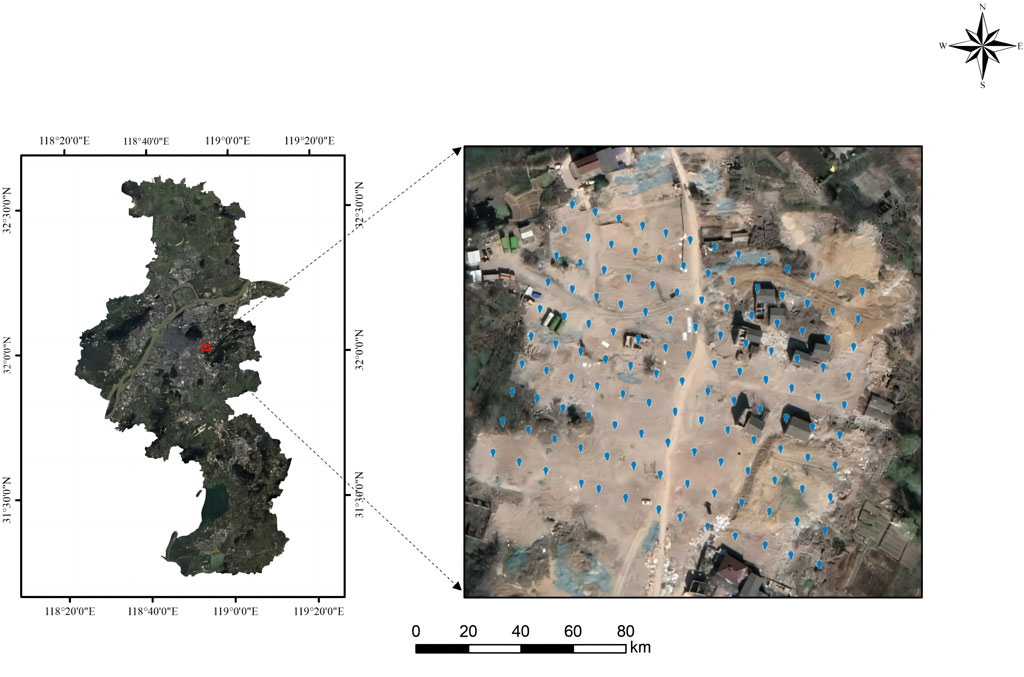
Figure 1. Overview map of the study area. The blue dots represent the locations of the drill holes.

2.2 Framework of the research methodology

The basic framework of the algorithm implementation, as depicted in Figure 2, is introduced in this section. The numbers in parentheses within the figure indicate the corresponding sections, and we will elaborate on the algorithm based on this procedural framework.

Figure 2

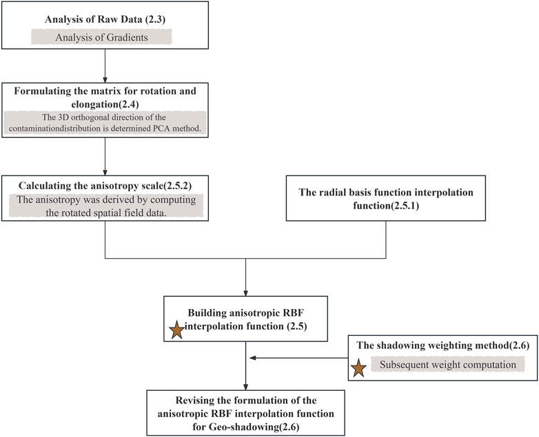
Figure 2. Algorithm flow chart. The five-pointed stars represent the innovative portions of this research.

Details of the methodology are provided below:

(1) In the step for analysis using raw data, experimental data points that meet the demands of the gradient method are obtained.

(2) In the step of formulating the rotation and elongation matrix, PCA is applied to the selected points to derive eigenvalues and eigenvectors, which are then used to construct the matrix. Thus, the local anisotropy characteristics can be expressed, and the shape of an ellipsoid that varies with the local data can be described.

(3) In the step for calculating the anisotropy scale and RBF interpolation, the anisotropic RBF interpolation can be constructed after modification of the RBF function.

(4) In the step for the shadowing weighting method, the points inside the ellipsoid are weighted twice, which improves the precision of the interpolation, and the formulation of the anisotropic RBF interpolation function for geo-shadowing is constructed.

2.3 Analysis of raw data

The gradient method was used to screen points with obvious characteristics of pollutants. The specific method was applied within a wide search space, in which the contamination value at each data point was used as a function of the value for that particular point. Because of the gridded structure of the dataset, isometric sampling allowed the estimation of the gradient of a data point through finite difference approximation along the respective dimension. For a given data point (i, j, k), an approximation of the gradient in the x direction can be obtained by utilizing the following (Eq. 1):

$\frac{\partial f}{\partial x}\approx \frac{f\left(i+1,j,k\right)-f\left(i-1,j,k\right)}{2\Delta x},(1)$

where Δx represents the distance between adjacent grids (isometric sampling in the x direction) and f is the contaminant function value. The same principle can be used to calculate gradients in the y and z directions. By calculating the approximation of the partial derivatives in each direction, the gradient vector of the data point can be obtained (∂f/∂x, ∂f/∂y, and ∂f/∂z). The trend threshold is set, and the points that satisfy the criteria are filtered.

2.4 Formulating the matrix for rotation and elongation

2.4.1 Practicability of the PCA method

PCA is a widely used statistical technique. Previous studies have primarily focused on employing PCA to conduct correlation analyses between variables. Buttafuoco et al. (2017) compared the PCA method with factorial Kriging analysis and concluded that although PCA is limited by the weak spatial correlation between variables, it is practical in trend analysis. Xiao et al. (2020) combined spatially weighted singularity mapping (SWSM) and PCA to predict the distribution of mineral resources in Hangzhou.

PCA is one of the most widely used data dimension reduction algorithms for determining a set of orthogonal axes for the original space. The largest proportion of variance is along the principal axis, followed by the sub-principal axis, and, lastly, the sub-axis. In this study, a rotation transformation matrix was determined by preserving all eigenvectors corresponding to the eigenvalues, such that the data from the original space could be projected into a space with large variance after the transformation to realize coordinate rotation. The search range can be obtained by calculating the stretch matrix with eigenvalues. By rotating and stretching the search space, we find more evenly distributed known points and overcome the problem of interpolation failure in local interpolation methods due to a lack of known interpolation points. A search ellipse is defined on the 2D plane to conform to the two-dimensional distribution of pollutants. The search ellipse is constructed because the points in the ellipse have a strong correlation with the points to be interpolated. The direction of pollutant distribution is consistent with the direction of the local ellipse axis, and the size of the ellipse is determined to facilitate the search for more sample points in the search ellipse. Finding more data points in the ellipse improves the fitting effect (Figure 3).

Figure 3

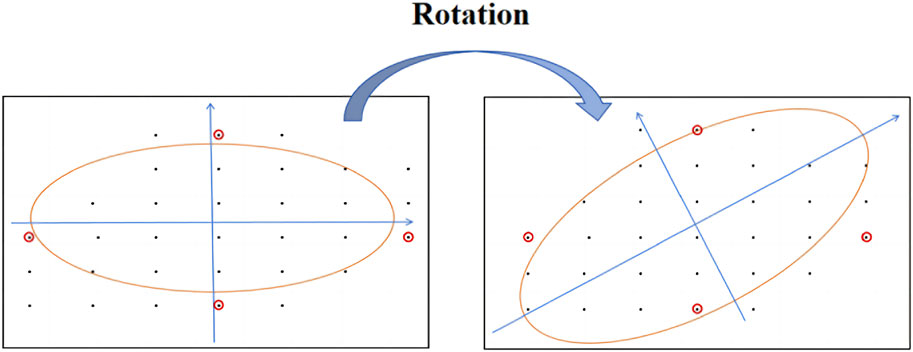
Figure 3. 2D elliptic rotation. Data points from the experiment are used for demonstration. In the neighborhood search in the 2D plane, the ellipse rotates to meet the 2D distribution of the contaminant, such that there are more points in the ellipse.

2.4.2 Implementation

2.4.2.1 Screening of raw data

Radial basis functions are accurate interpolation methods in which the curve of the function encompasses every known point. However, points with low contamination changes are not conducive to finding the direction of change, and it is difficult to reflect the spatial variability of pollutants at the data level. Therefore, we use the gradient idea from Section 2.4.1 to filter the data.

2.4.2.2 Establishment of the matrix for construction of covariance matrix

Searching for sample points is performed within a local range, specifically for n data samples, each containing three variables (x,y,z), which constitute the following matrices. Here, n is the local search for the drilling sample data within the ellipsoid (Eqs. (2) and (3)):

$X=\left[\begin{array}{ccc}{x}_{11}& x_{12}& x_{13}\\ x_{21}& x_{22}& x_{23}\\ ⋮& ⋮& ⋮\\ x_{n1}& x_{n2}& x_{n3}\end{array}\right].(2)$

The data samples for constructing the variance-covariance matrix were averaged by row. The covariance matrix is built to calculate the amount of covariance and correlation in a given geographic area. It explains how changes in one set of geographical variables occur at the same time as changes in another.

${\mathrm{\Sigma }}_x=\left[\begin{array}{ccc}\text{cov}\left(x_1,x_1\right)& \text{cov}\left(x_1,x_2\right)& \text{cov}\left(x_1,x_3\right)\\ \text{cov}\left(x_2,x_1\right)& \text{cov}\left(x_2,x_2\right)& \text{cov}\left(x_2,x_3\right)\\ \text{cov}\left(x_3,x_1\right)& \text{cov}\left(x_3,x_2\right)& \text{cov}\left(x_3,x_3\right)\end{array}\right].(3)$

2.4.2.3 Obtaining eigenvalues and feature vectors

${\lambda }_1,{\lambda }_2,{\lambda }_3$ are the eigenvalues determined by the following (Eq. 4),

$Av=\lambda v,(4)$

to obtain the feature vector $v=\left[\overrightarrow{v_1},\overrightarrow{v_2},\overrightarrow{v_3}\right].$

2.4.2.4 Elongation and rotation matrices

The elongation and rotation matrices were defined as follows Eqs (5), (6), (7):

Elongation coefficient:

$k=0.5*\left({\lambda }_{\min }/{\lambda }_{\max }\right)(5)$

Elongation matrix:

$L=\left[\begin{array}{ccc}1& 0& 0\\ 0& 1& 0\\ 0& 0& k\end{array}\right](6)$

Rotation matrix:

$R=\left[\overrightarrow{v_1},\overrightarrow{v_2},\overrightarrow{v_3}\right](7)$

${\lambda }_{\min }$ is the minimum eigenvalue sought and ${\lambda }_{\max }$ is the maximum eigenvalue sought. ${\overrightarrow{v}}_i$ is the ith eigenvector.

2.4.2.5 Combined matrix

The rotation and the elongation matrices were combined into an operation transformation matrix M as follows (Eq. 8):

$M=L\cdot R.(8)$

The covariance matrix constructed in the PCA analysis is symmetric, and the eigenvectors obtained are orthogonal. The data are transformed based on these eigenvectors. The orthogonality principle dictates that only rotation is present without any dimension reduction. The PCA method was employed to derive the characteristics of the pollutant distribution in the anisotropic direction within the geographic 3D space. Finally, we obtained the variable range in each direction by calculating the variance function and integrating it into the stretching matrix to determine the variable range of the anisotropy.

2.5 Building the anisotropic RBF interpolation function

2.5.1 RBF interpolation

The methodology outlined in Section 2.4 describes the process of identifying the three principal spatial directions of the pollutant, with the RBF serving as an accurate interpolation method (Ping, 2018). The basis function types are shown in Table 1. Thus, N data samples were selected, and the following function was assumed (Eq. 9):

$f\left(x\right)={\displaystyle \sum _i^N}{C}_i\rho \left({‖\left(x-x_i\right)‖}_2\right),(9)$

where $C_i$ is the weight, f(x) is the concentration of pollutants at a certain point in the soil, ${‖x-x_i‖}_2$ is the Euclidean distance between the interpolation point and the known point, and $\rho \left({‖x-x_i‖}_2\right)$ is a basis function. The main types of basis functions (Aràndiga et al., 2020) are shown in Table 1. We employed the monomial function as the basis for our experiments. This function is better suited to non-uniformly distributed data points and can provide more accurate interpolation results for functions with significant local changes.

Table 1

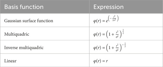
Table 1. Types of basis functions.

2.5.2 Calculating the anisotropy scale

In this study, the spatial scale of the pollution distribution in all directions was determined by analyzing its spatial variation, as inspired by the estimation by Sun et al. (2019) of the soil pollution value in the field. The expression of anisotropy is thus formulated. We aim to improve the accuracy of the pollutant prediction and transform the radial basis function to develop an anisotropic property.

The rotation matrices constructed by the anisotropic RBF stem from the PCA analysis of the 3D coordinates of the data points, where the rotation matrix is the eigenvector, and the stretching matrix is related to the eigenvalues. In the geographical 3D space, the position coordinate RBF model of Casciola et al. (2006) was modified, and the RBF interpolation model considering the anisotropic features of the 3D space field was constructed.

The stretching and rotation of the radially symmetric RBF basis functions were as follows: From b to e, only the influence of spatial position on the interpolation model is used; the influence of the pollutant attribute value on the model is not used. Therefore, we conducted a gradient analysis at each interpolation node and screened the points with large changes in the surrounding attribute values for model fitting. In particular, step f is our improvement:

a) Node anisotropic RBF interpolation function (Eq. 10):

$F\left(x,y,z\right)={\displaystyle \sum _{k=1}^n}{w}_k\left(x,y,z\right)S_k\left(x,y,z\right)(10)$

$S_k\left(x,y,z\right)$ is an expression for RBF, and $w_k\left(x,y,z\right)$ is the weight. k is an unknown point in spatial data.

b) Define the local search region for the point of k to be interpolated $x_k$: Local reference points were selected to find the covariance matrix $c_{\left(x_k\right)}$, and the diagonal matrix of the eigenvalues ∧ was constructed. The eigenvalues were ${\lambda }_1>{\lambda }_2>{\lambda }_3$, and the eigenvector corresponding to the value of $c_{\left(x_k\right)}$ was $V=\left({\overrightarrow{v}}_1,{\overrightarrow{v}}_2,{\overrightarrow{v}}_3\right)$.

c) Custom T norm (Eq. 11):

$T_k={\lambda }_{\underset{c\left(x_k\right)}{\max }}{C}^{-1}\left({\mathbf{x}}_k\right)={\lambda }_{\underset{c\left(x_k\right)}{\max }}{V}_k{\mathrm{\Lambda }}_k^{-1}{V}_k^T.(11)$

  ${\lambda }_{\underset{c\left(x_k\right)}{\max }}$ is the largest eigenvalue obtained from the covariance matrix constructed with a local reference point k.

d) Transform the node RBF to (Eq. 12)

$S=S\left(\mathbf{x}\right)={\displaystyle \sum _{k=1}^N}{c}_k\varphi \left(\parallel \left({\mathbf{x}}_k-\mathbf{x}\right){\parallel }_T\right)(12)$

e) Compute the M matrix as follows (Eqs 13, 14, 15), which facilitates later calculations by (Eq. 8):

$M=L\cdot R=\sqrt{{\lambda }_{\underset{c\left(x_k\right)}{\max }}}\cdot \sqrt{{\mathbf{\Lambda }}^{-1}}\cdot V^T,(13)$

${\lambda }_{\underset{c\left(x_k\right)}{\max }}=\frac{1}{2}{\lambda }_1,(14)$

$\parallel \mathbf{x}{\parallel }_T=\sqrt{{\mathbf{x}}^{T}T\mathbf{x}}=\sqrt{{\mathbf{x}}^T{\mathbf{M}}^T\text{Mx}}=\parallel \mathrm{M}\mathrm{x}{\parallel }_2.(15)$

f) Replacing $S\left(\mathbf{x}\right)$ with $f_{T_k}\left(x,y,z\right)$, an anisotropic radial basis function is obtained (Eqs 16, 17):

$F\left(x,y,z\right)={\displaystyle \sum _{k=1}^n}{w}_k\left(x,y,z\right)f_{T_k}\left(x,y,z\right),(16)$

$\begin{array}{c}{f}_{T_k}\left(x,y,z\right)=f_{T_k}\left(\mathbf{x}\right)={\displaystyle \sum _{k=1}^N}{c}_k\varphi \left(\parallel \left({\mathbf{x}}_k-\mathbf{x}\right){\parallel }_{T_k}\right)\\ X_{T_k}=\parallel R\cdot L_k\cdot x{\parallel }_2\\ L_k=\left[\begin{array}{ccc}{h}_x^{\prime }/\max \left(h_x^{\prime },h_y^{\prime },h_z^{\prime }\right)& 0& 0\\ 0& h_y^{\prime }/\max \left(h_x^{\prime },h_y^{\prime },h_z^{\prime }\right)& 0\\ 0& 0& h_z^{\prime }/\max \left(h_x^{\prime },h_y^{\prime },h_z^{\prime }\right)\end{array}\right].\end{array}(17)$

The above is the anisotropic RBF interpolation model. The RBF function varies from the node RBF function jointly by the rotation matrix (R) and the stretching matrix ($L_k$). It finds the influence range of the three directions (h´_x, h´_y, and h´_z) and, finally, the change range of the three directions. The rate of variation in the three directions is set to form the diagonal matrix. In terms of the fitting weights, weighting by grouping distance is more efficient for pollutant distribution (Eq. 18):

$w_i=h_i/h_{all},(18)$

where $h_i$ is the current grouping distance and $h_{all}$ is the sum of all grouping distances. The inherent properties of pollutants imply that when the distance is smaller, the spatial correlation and the weight are greater.

$F\left(x,y,z\right)={\displaystyle \sum _{k=1}^n}{w}_k\left(x,y,z\right)f_{T_k}\left(x,y,z\right).(19)$

2.6 Revising the formulation of the anisotropic RBF interpolation function for geo-shadowing

The above studies were only spatially interpolated in terms of data and did not consider the impact of real geographic space. In contrast, spatial fitting of the data for known and interpolated points (unknown points) relies on the correlation between Euclidean distance and pollution distribution, where the surrounding pollutant locations (direction) and pollution values impact the pollutant distribution. The influence is informed by relevant geoscientific experience; thus, (Eq. 19) is adjusted to establish the correlation between pollution value and spatial position through quadratic weight determination. We refer to this quadratic weight as the “geographic shading coefficient.” A detailed explanation is provided below. Figure 4 shows that the included angle between Point 3 and Point 2 concerning the interpolation Point 0 is narrow and that the influence of Point 2 on the interpolation Point 0 is more prominent than that of Point 3. In this context, Point 2 would have some protection from Point 3. The larger values observed for the other points of each angle lead us to believe that either no geographic shading is present or that the impact of geographic shading is minimal.

Figure 4

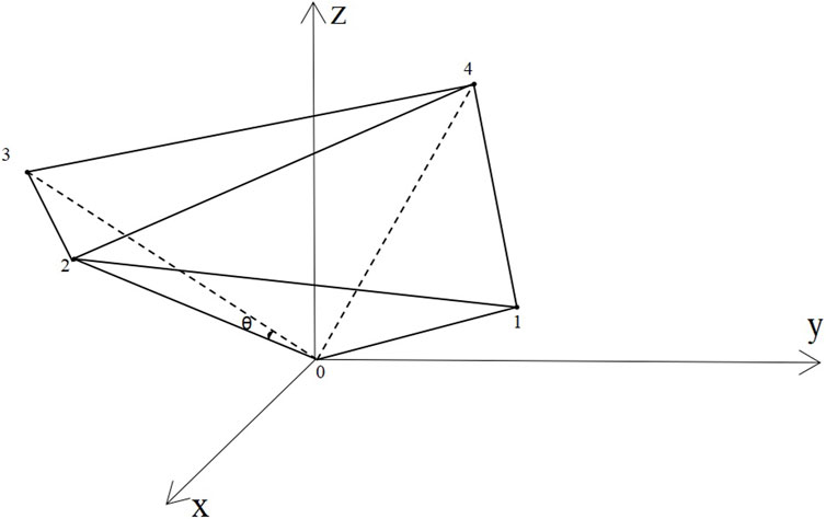
Figure 4. Spatial occlusion. Spatial relationship between known points and points to be interpolated.

The space angle is calculated in a manner similar to that of two dimensions. When calculating the angle between two vectors, the dot product operation can be used to determine the relationship between them and convert it to the angle value through the inverse cosine (arccos) function. The dot product of two vectors, A and B, can be computed in 3D using the following (Eq. 20)

$A•B=\left|A\right|\times \left|B\right|\times \cos \theta ,(20)$

where |A| and |B| represent the length of vectors A and B and $\theta$ represents the angle between them. According to the above (Eq. 20), we can find the value of $\theta$ (Eq. 21).

$\theta =arc\left(A•B/\left(\left|A\right|\times \left|B\right|\right)\right).(21)$

The number of sample points will depend on the search ellipsoid constructed, and the points in the ellipsoid will all be used for interpolation calculations of unknown points.

The following formula is used to calculate masking Eqs (22), (23):

$L_{ij}=\left\{\begin{array}{ll}1& {\alpha }_{ij}\ge 360°/m\\ {\sin }^r{\theta }_{ij}={\left(1-{\cos }^2{\theta }_{ij}\right)}^{\frac{r}{2}}& {\alpha }_{ij}<360°/m\end{array}\right.,(22)$

$w_i^{\prime }=\left\{\begin{array}{l}1\\ {\prod }_{j=1}^{j=i-1}{L}_{ij}\end{array}\right.\begin{array}{cc}& \begin{array}{c}i=1\\ i=2,3,...,m\end{array},\end{array}(23)$

where $m$ represents the number of sample points in an ellipsoid search, $L_{ij}$ represents the shadowing degree of sample point j to sample point i, and ${\theta }_{ij}$ is the angle between any two points in space and the interpolation point.

The calculation method used as pseudocode:

(1) Statistics indicate that the number of points in the ellipsoid search is $m$.

(2) A depth-first search is conducted, and the angle between sample points and interpolation points is calculated and stored in the container.

(3) The values in the container are calculated.

$F\left(x,y,z\right)={\displaystyle \sum _{k=1}^n}{w}_k^{\prime }{w}_k\left(x,y,z\right)f_{T_k}\left(x,y,z\right).(24)$

2.7 Precision analysis

The precision and robustness of interpolation methods under various basis functions were compared to evaluate the robustness of the empirical shadowing weighted anisotropy RBF models and methods. To this end, the Kriging interpolation and RBF interpolation methods were utilized in the comparative validation. Furthermore, the following statistical metrics were used to evaluate the precision: minimum (MIN), maximum (MAX), mean (ME), and root mean square error (RMSE) (Ahn and Lee, 2022). Furthermore, the determination coefficient (R²) is used to represent the fitting degre. The corresponding formulae for calculating these statistical metrics, where Z is the true value, z is the estimated value, $\overline{Z}$ is the average value, n is the interpolation point, and the error was as follows (Eq. 25):

$\epsilon =Z-z.(25)$

The minimum error expression (Eq. 26):

$\mathrm{MIN}=\min \left(\left|{\epsilon }_i\right|\right),i=1,\dots ,n(26)$

The maximum error expression (Eq. 27):

$\mathrm{MAX}=\max \left(\left|{\epsilon }_i\right|\right),i=1,\dots ,n(27)$

The expression of mean error (Eq. 28):

$\text{ME}={\displaystyle \sum _{i=1}^n}\left|{\epsilon }_i\right|/n,i=1,\dots ,n(28)$

The root mean square error (Eq. 29):

$\text{RMSE}=\sqrt{{\displaystyle \sum _{i=1}^n}{\epsilon }_i^2/n,}i=1,\dots ,n(29)$

The determination coefficient (Eq. 30):

$R^2=\mathbf{1}-\frac{\sum {\left({\mathrm{Z}}_i-z_i\right)}^2}{\sum {\left(Z_i-\overline{Z}\right)}^2}(30)$

3 Results and discussion

3.1 PCA interpretation of results

Some sample points in a search ellipsoid are shown in Table 2 for illustration. The first column of the table is the borehole ID. The X column is the east coordinate, the Y column is the north coordinate, the Z column is the elevation, and the C column is the toluene pollutant content (mg/Kg). Points with higher pollutant concentrations were chosen for the argument. The matrix formula is shown in (Eq. 31):

$\left[\begin{array}{ccc}512273.8183& 3360129.992& 3.15\\ 512342.9062& 3360130.07& 2.405\\ 512273.8957& 3360061.248& 2.89\\ 512342.984& 3360061.326& 2.12\\ 512412.0724& 3360061.405& 2.298\\ 512273.7409& 3360198.734& 2.56\\ 512342.8283& 3360198.812& 2.53\\ 512273.8183& 3360129.992& 2.15\\ 512342.9062& 3360130.07& 1.405\\ 512273.8957& 3360061.248& 1.89\\ 512342.984& 3360061.326& 1.12\\ 512273.7409& 3360198.734& 1.56\end{array}\right].(31)$

Table 2

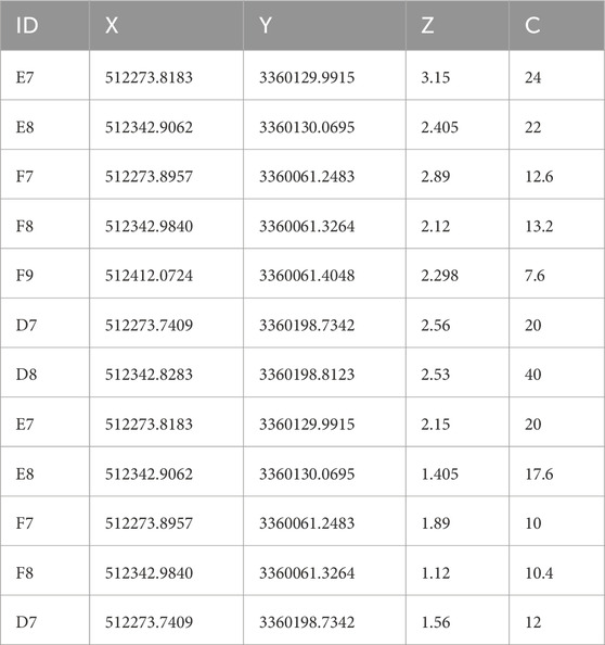
Table 2. Local interpolation points.

We show the data graph to better explain PCA rotation. Figure 5A shows the original data effect, and Figure 5B shows the data distribution after PCA rotation.

Figure 5

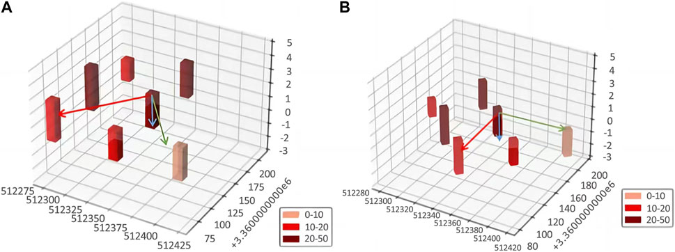
Figure 5. (A) Original spatial location. (B) The position in space after rotation. The axis shows the three main directions of pollutant distribution.

3.2 Analysis of the variogram of contaminated areas

The distribution direction of pollutants was calculated above, and the axis length of the ellipsoid in three directions was determined by calculating the variation function to determine the shape of the ellipsoid. In addition, Figure 6 shows the variogram analysis of pollutant concentrations in the X-axis, Y-axis, and Z-axis in a local range, and the boxes in the figure are sample data. When the distance is below 207 m on the X-axis, the curvature gradually increases due to the small distance. Beyond 207 m, the curvature flattens. At 276.35 m, the curve tends to be parallel to the X-axis. The variogram curve shows increased steepness around 207 m, indicating a significant spatial correlation within this range. Therefore, with a total variable range of 414.53, it is feasible to use the semi-variable range as the range calculated for the X-axis direction of the model. A significant change in curvature occurs at the abscissa of 206.29 m in the Y-axis. At approximately 155 m, there is a pronounced curvature and spatial correlation, making it feasible to select the semi-variable range as the search range in the Y-axis direction. On the Z-axis, the curvature undergoes significant changes after 1.98 m, with notable curvature and high spatial correlation near 1.5 m. Therefore, the semi-variance is utilized as the search range in the Z-axis direction.

Figure 6

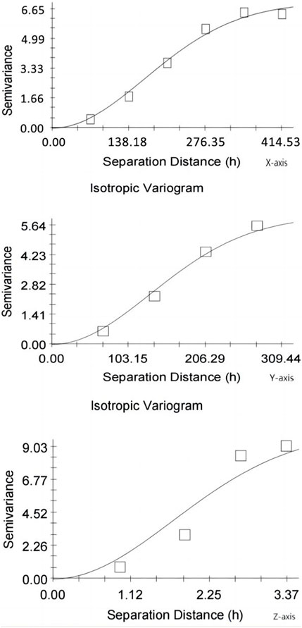
Figure 6. Variogram of the X, Y, and Z-axes.

The residual sum of squares (RSS) served as a metric for assessing the correlation between the independent and dependent variables. Fundamentally, a smaller RSS value indicates a stronger spatial correlation. The coefficient of certainty (R²) was used to estimate the goodness of fit of the regression equation. Variogram analysis revealed regional anisotropy in the distribution of soil pollutants, as summarized in Table 3 (RSS is the sum of squared residuals. When the value of the semivariogram changes from the nugget value to the sill value, the distance between sampling points is called the range, that is, “a”).

Table 3

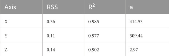
Table 3. X, Y, and Z variogram fitting analysis.

3.3 Analysis of the precision of contaminated areas

To assess the accuracy of the method, this section evaluates the fitting effect of the model and the precision of the data. The Kriging and RBF methods were selected for comparative validation. The specific approach involves removing the known points one by one for spatial interpolation. Each model is then evaluated based on criteria such as MIN, MAX, ME, RMSE, and R2, calculated from the comparison between true values and estimated values to determine the reliability of the model.

3.3.1 Analysis of the precision of 2D spatial interpolation for geo-shadowing weighted anisotropy RBF-PCA

In this study, a stratum with a sampling depth of 1 m was selected for two-dimensional precision analysis, as shown in Table 4.

Table 4

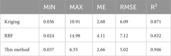
Table 4. 2D accuracy analysis of 130 sample points.

We selected 130 samples from the soil layer at the 1 m depth. Comparing the RMSE values, it is noticeable that the RMSE (6.09) for Kriging does not change much with the RBF (7.12) value. Conversely, the performance of the method proposed in this article exhibits a slightly improved RMSE at 5.02 compared to the other methods. This is because the proposed method uses a local interpolation method, and more points can be searched for spatial fitting by rotation. In the fitting of extreme points, when the observed value is 25.6 mg/kg, the fitting effect of the proposed method is 19.2, which is significantly better than that of RBF (10.62) and Kriging (13.76) (Figure 7). Furthermore, the R² of the linear regression between the observed and estimated values calculated are Kriging (0.871), RBF (0.832), and the proposed method (0.946).

Figure 7

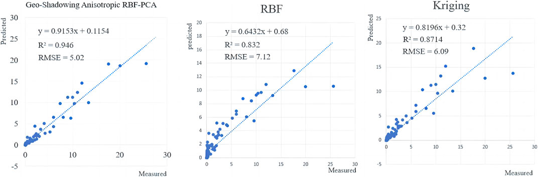
Figure 7. Precision analysis plot of the 2D interpolation method.

The 2D graph (Figure 8) illustrates a gradual decrease in pollutant concentration from the central value of 24.5 mg/kg to a level below 0.011 mg/kg. The fitting effect of the proposed method is notably smooth, devoid of any fitting cavities. The region exhibiting a high concentration of pollutants within the field corresponds to the waste treatment zone of the plant. This figure effectively illustrates the distribution range of pollutants in the soil.

Figure 8

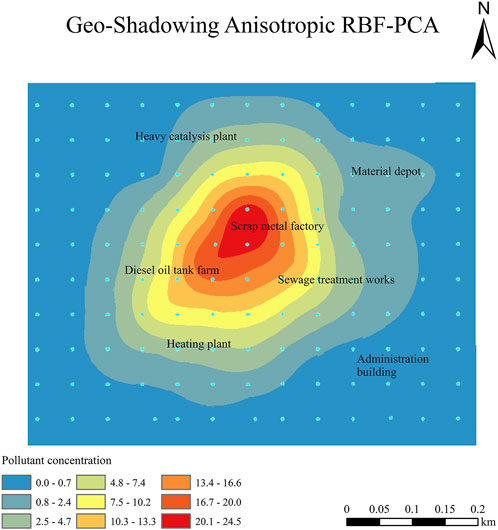
Figure 8. 2D interpolation of toluene contaminants for 130 sample points.

3.3.2 Evaluating the analysis of 3D spatial interpolation for empirical shadowing weighted anisotropy RBF

The precision assessment of 3D spatial interpolation was performed utilizing only vertical depth data. The main arguments were demonstrated by point-by-point interpolation, as shown in Table 5.

Table 5

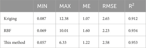
Table 5. 3D precision analysis.

Through the analysis of 3D data and the comparison of RMSE, it can be seen that the RMSE of the proposed method in 3D space (2.58) is still better than that of Kriging (2.65). This is because the anisotropic ellipsoid in the proposed method in 3D space can change shape with the change of sample space. Thus, more known points conforming to interpolation are searched. In geospatial contexts, the involvement of a greater number of reasonable points in estimating an unknown point is a key factor in improving the RMSE evaluation metric. At the same time, the directionality in 3D space is more diverse, and the weight distribution of geoscience direction plays an important role. This enables further quantification of the varying degrees of influence each known point has on an unknown point, thereby enhancing the RSME evaluation metric. Compared with the RMSE in 2D space, the fitting effect of 3D is better because there are more data points in 3D space. In the analysis of extreme points, when the observed value is 40 mg/kg, it is consistent with the 2D situation because the change of pollutants near the extreme points is relatively large. The R² in three dimensions is 0.912 for Kriging, 0.934 for RBF, and 0.953 for the proposed method (Figure 9).

Figure 9

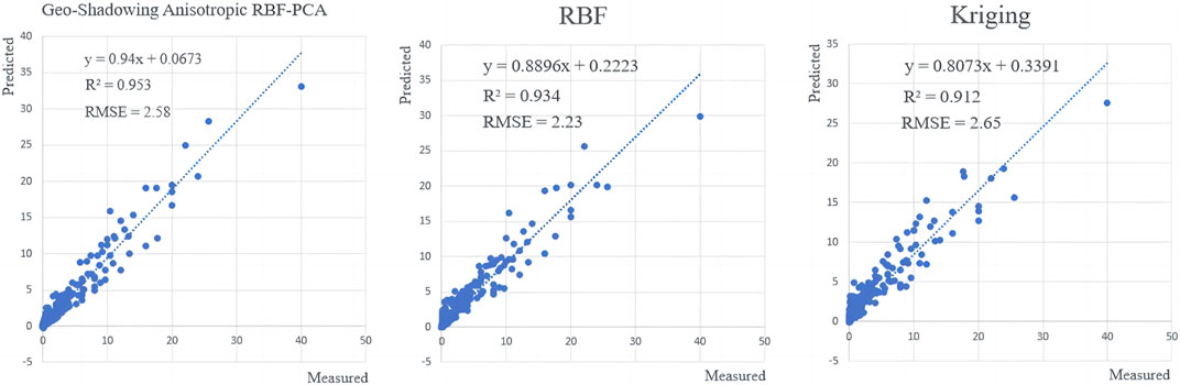
Figure 9. Precision analysis plot of the 3D interpolation method.

As shown in Figure 10, by cutting the contaminated object along the main axis, we learned that the cell body of a pollutant at the waste site could contain a high concentration of pollutant in this area. The vertical profile display offers a more comprehensive representation of the pollutant distribution state, revealing a maximum pollution value of 40 mg/kg at the surface that gradually decreases to 2.23 mg/kg with increasing depth. This process at hand does not follow a linear or conventional function reduction approach. Within this reduction process, the lithology of the soil from the surface down to filling, silt, silt sand, and clay plays a significant role in determining soil porosity and other related factors. Overall, the two cases mentioned earlier suggested that combining anisotropy based on accurate interpolation and the introduction of geological experience to better allocate the weight of data improves the precision of the results. In Figure 10, for the sake of intuitive data analysis, after interpolation, we expanded the Z-axis by a factor of 70 during the image display phase.

Figure 10

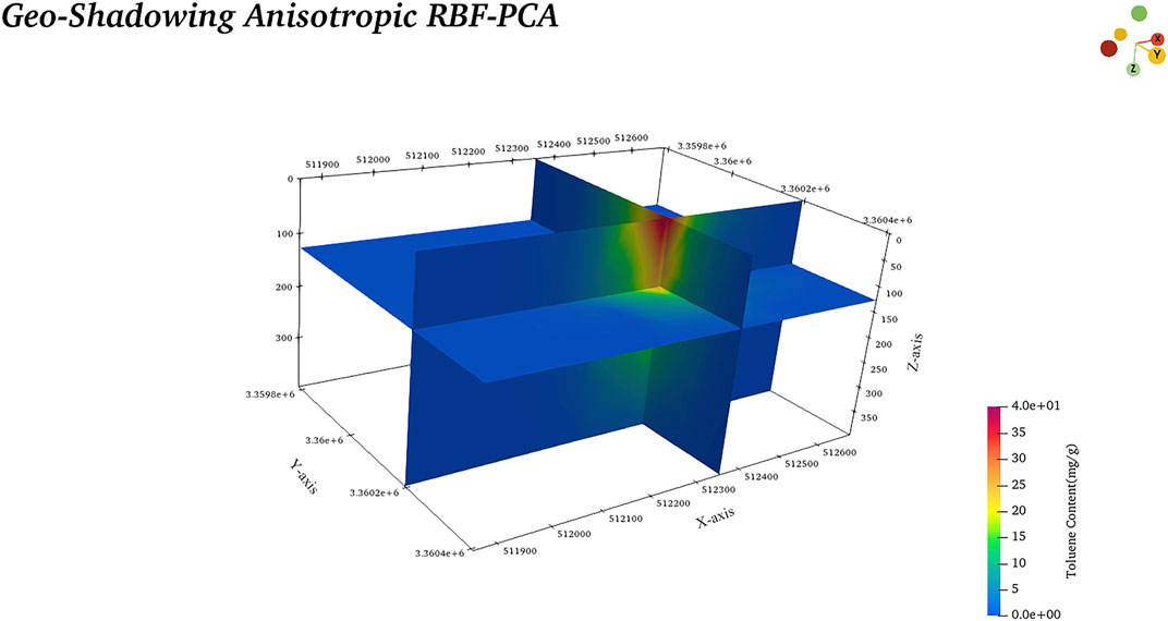
Figure 10. 3D interpolation of toluene contaminants for 650 sample points.

4 Conclusion

In this study, the RBF function was integrated with PCA to redefine the local anisotropy, which varied within the sample space in the form of an ellipsoid. The directional characteristics of geoscience are introduced to improve the accuracy of the algorithm. We called it the geo-shadowing anisotropic RBF-PCA method.

For the 2D space, the RMSE values of Kriging, RBF, and the proposed method are 6.09, 7.12, and 5.02, respectively. In the interpolation results, the proposed method had better spatial continuity, smoothness, and higher feasibility. For the 3D space, the RMSE values of Kriging, RBF, and the proposed method are 2.65, 2.23, and 2.58, respectively. The latter also has high reliability.

Data availability statement

The original contributions presented in the study are included in the article/supplementary material; further inquiries can be directed to the corresponding author.

Author contributions

XW: writing–original draft. RG: investigation and writing–review and editing. JL: investigation and writing–review and editing. MS: data curation and writing–review and editing. JL: formal analysis and writing–review and editing. DZ: funding acquisition, investigation, and writing–review and editing. FZ: investigation and writing–review and editing. QL: investigation and writing–review and editing.

Funding

The author(s) declare that no financial support was received for the research, authorship, and/or publication of this article. This research did not receive any specific grant from funding agencies in the public, commercial, or not-for-profit sectors.

Acknowledgments

The authors would like to thank all the above authors for their contributions and their two teachers for their guidance (Bo Wang and Huan Liu).

Conflict of interest

Author MS was employed by Jiangsu Hi-Target Navigation Tech Co., Ltd.

The remaining authors declare that the research was conducted in the absence of any commercial or financial relationships that could be construed as a potential conflict of interest.

Publisher’s note

All claims expressed in this article are solely those of the authors and do not necessarily represent those of their affiliated organizations, or those of the publisher, the editors, and the reviewers. Any product that may be evaluated in this article, or claim that may be made by its manufacturer, is not guaranteed or endorsed by the publisher.

References

Ahn, J., and Lee, Y. (2022). Ordinary kriging of daily mean SST (sea surface temperature) around South Korea and the analysis of interpolation accuracy. J. Korean Soc. Surv. Geod. Photogramm. Cartogr. 40, 51–66. doi:10.7848/KSGPC.2022.40.1.51

CrossRef Full Text | Google Scholar

Aràndiga, F., Donat, R., Romani, L., and Rossini, M. (2020). On the reconstruction of discontinuous functions using multiquadric RBF–WENO local interpolation techniques. Math. Comput. Simul. 176, 4–24. doi:10.1016/j.matcom.2020.01.018

CrossRef Full Text | Google Scholar

Brito, W. B. M., Campos, M. C. C., de Souza, F. G., Silva, L. S., da Cunha, J. M., de Lima, A. F. L., et al. (2022). Spatial patterns of magnetic susceptibility optimized by anisotropic correction in different Alisols in southern Amazonas, Brazil. Precis. Agric. 23, 419–449. doi:10.1007/s11119-021-09843-6’

CrossRef Full Text | Google Scholar

Buttafuoco, G., Guagliardi, I., Tarvainen, T., and Jarva, J. (2017). A multivariate approach to study the geochemistry of urban topsoil in the city of Tampere, Finland. J. Geochem. Explor. 181, 191–204. doi:10.1016/j.gexplo.2017.07.017

CrossRef Full Text | Google Scholar

Carr, J. C. (2001). Reconstruction and representation of 3D objects with radial basis functions. in Proc. of the 28th Annual Conf. on Computer Graphics and Interactive Techniques. New York, NY, US, ACM, 67–76.

CrossRef Full Text | Google Scholar

Casciola, G., Lazzaro, D., Montefusco, L. B., and Morigi, S. (2006). Shape preserving surface reconstruction using locally anisotropic radial basis function interpolants. Comput. Math. Appl. 51, 1185–1198. doi:10.1016/j.camwa.2006.04.002

CrossRef Full Text | Google Scholar

Chilès, J. P. (2012). Geostatistics: modeling spatial uncertainty. second ed. New York: John Wiley & Sons.

Google Scholar

Cuomo, S., Galletti, A., Giunta, G., and Marcellino, L. (2017). Reconstruction of implicit curves and surfaces via RBF interpolation. Appl. Numer. Math. 116, 157–171. doi:10.1016/j.apnum.2016.10.016

CrossRef Full Text | Google Scholar

Ding, Q., Wang, Y., and Zhuang, D. (2018). Comparison of the common spatial interpolation methods used to analyze potentially toxic elements surrounding mining regions. J. Environ. Manage. 212, 23–31. doi:10.1016/j.jenvman.2018.01.074

PubMed Abstract | CrossRef Full Text | Google Scholar

Fasshauer, G. F. (2007). Meshfree approximation methods with MATLAB 9812706348 (River Edge, NJ: World Scientific Publishing).

Google Scholar

Franke, R. (1982). Scattered data interpolation: tests of some methods. Math. Comp. 38, 181–200. doi:10.1090/S0025-5718-1982-0637296-4

CrossRef Full Text | Google Scholar

Gao, Y., Guo, J., Wang, J., and Lv, X. (2022). Assessment of three-dimensional interpolation method in hydrologic analysis in the East China Sea. J. Mar. Sci. Eng. 10, 877. doi:10.3390/jmse10070877

CrossRef Full Text | Google Scholar

Hou, Y., Li, Y., Tao, H., Cao, H., Liao, X., and Liu, X. (2023). Three-dimensional distribution characteristics of multiple pollutants in the soil at a steelworks mega-site based on multi-source information. J. Hazard. Mater. 448, 130934. doi:10.1016/j.jhazmat.2023.130934

PubMed Abstract | CrossRef Full Text | Google Scholar

Levasseur, P., Erdlenbruch, K., and Gramaglia, C. (2021). The health and socioeconomic costs of exposure to soil pollution: evidence from three polluted mining and industrial sites in Europe. J. Public Health 30, 2533–2546. doi:10.1007/s10389-021-01533-x

CrossRef Full Text | Google Scholar

Li, S., Xi, W., Li, C., and Bi, T. (2020). Study on pollutant model construction and three-dimensional spatial interpolation in soil environmental survey. IOP Conf. Ser. Earth Environ. Sci. 467, 012154. doi:10.1088/1755-1315/467/1/012154

CrossRef Full Text | Google Scholar

Macêdo, I., Gois, J. P., and Velho, L. (2009). Hermite interpolation of implicit surfaces with radial basis functions Brazilian Symposium on Computer Graphics and Image Processing (SIBGRAPI), XXII, 1–8. doi:10.1109/SIBGRAPI.2009.11

CrossRef Full Text | Google Scholar

Maksimova, Y. G., Maksimov, A. Y., and Demakov, V. A. (2018). Biotechnological approaches to the bioremediation of an environment polluted with trinitrotoluene. Appl. Biochem. Microbiol. 54, 767–779. doi:10.1134/S0003683818080045

CrossRef Full Text | Google Scholar

Mrao, S., Joshua, R. E., and Rekapalli, M. (2020). Batch-scale remediation of toluene contaminated groundwater using PRB system with tyre crumb rubber and sand mixture. J. Water Process Eng. 35, 101198. doi:10.1016/j.jwpe.2020.101198

CrossRef Full Text | Google Scholar

Ping, D. (2018). Spatial interpolation model of three-dimensional spatial anisotropy radial basis function. (Nan Jing: Nanjing Normal University).

Google Scholar

Qiao, P., Li, P., Cheng, Y., Wei, W., Yang, S., Lei, M., et al. (2019). Comparison of common spatial interpolation methods for analyzing pollutant spatial distributions at contaminated sites. Environ. Geochem. Health. 41, 2709–2730. doi:10.1007/s10653-019-00328-0

PubMed Abstract | CrossRef Full Text | Google Scholar

Rao, S. M., Joshua, R. E., and Rekapalli, M. (2020). Batch-scale remediation of toluene contaminated groundwater using PRB system with tyre crumb rubber and sand mixture. J. Water Process Eng. 35, 101198. doi:10.1016/j.jwpe.2020.101198

CrossRef Full Text | Google Scholar

Skala, V. (2010). Progressive RBF interpolation. in Proceedings of the 7th International Conference on Computer Graphics, Virtual Reality, Visualisation and Interaction in Africa. New York, NY, US, 17–20.

CrossRef Full Text | Google Scholar

Smolyar, I., Bromage, T., and Wikelski, M. (2016). Quantification of layered patterns with structural anisotropy: a comparison of biological and geological systems. Heliyon 2, e00079. doi:10.1016/j.heliyon.2016.e00079

PubMed Abstract | CrossRef Full Text | Google Scholar

Sun, X. L., Wu, Y. J., Zhang, C., and Wang, H. (2019). Performance of median kriging with robust estimators of the variogram in outlier identification and spatial prediction for soil pollution at a field scale. Sci. Total Environ. 666, 902–914. doi:10.1016/j.scitotenv.2019.02.231

PubMed Abstract | CrossRef Full Text | Google Scholar

Tao, H., Liao, X., Cao, H., Zhao, D., and Hou, Y. (2022). Three-dimensional delineation of soil pollutants at contaminated sites: progress and prospects. J. Geogr. Sci. 32, 1615–1634. doi:10.1007/s11442-022-2013-6

CrossRef Full Text | Google Scholar

Xiao, F., Wang, K., Hou, W., and Erten, O. (2020). Identifying geochemical anomaly through spatially anisotropic singularity mapping: a case study from silver–gold deposit in Pangxidong district, SE China. J. Geochem. Explor. 210, 106453. doi:10.1016/j.gexplo.2019.106453

CrossRef Full Text | Google Scholar

Yang, R., and Xing, B. (2021). A Comparison of the performance of different interpolation methods in replicating rainfall magnitudes under different climatic conditions in Chongqing Province (China). Atmosphere 12, 1318. doi:10.3390/atmos12101318

CrossRef Full Text | Google Scholar

Zhang, H., and Wang, X. S. (2020). The impact of groundwater depth on the spatial variance of vegetation index in the Ordos Plateau, China: a semivariogram analysis. J. Hydrol. 588, 125096. doi:10.1016/j.jhydrol.2020.125096

CrossRef Full Text | Google Scholar

Zhengquan, L. (2015). Inverse distance weight interpolation that takes into account directional occlusion. Surv. Mapp. 44, 91–98. doi:10.11947/j.AGCS.2015.20130349

CrossRef Full Text | Google Scholar