 Weicheng Gong
 Huayuan Chen2
- 1School of Transport and Civil Engineering, Fujian Agriculture and Forestry University, Fuzhou, China
- 2Fujian Earthquake Agency, Fuzhou, China
- 3Zhejiang Earthquake Agency, Hangzhou, China
- 4Department of Civil Engineering and Architecture, Wuyi University, Wuyishan, China
Seismic b-value is one of the most important parameters for seismological research and seismic hazards assessment, while the accuracy of the b-value largely depended on the completeness of seismic catalog. This article compares eight methods for estimating the minimum magnitude of completeness (Mc). The results indicate that the modified maximum curvature method (MMAXC), exhibits greater stability and accuracy, closely approximating the standard Mc obtained from the synthetic seismic catalogs. We then calculate the b-value using the instrumental seismic catalog from 2000–2023 in the eastern Tibetan Plateau. The results indicate that the five major earthquakes occur in regions with lower b-value. In addition, the temporal evolution of b-value before and after major earthquakes exhibits a common trend of decreasing before earthquakes, and increasing after earthquakes, which may reflect the stress accumulation and release during earthquakes. Combining the results of maximum shear strain rate and b-value, we identify five regions characterized by low b-value and high shear strain rate, indicating a higher potential seismic hazard in the future.
1 Introduction
The relationship between the magnitude and frequency of earthquakes embodies a fundamental seismic principle. This statistical relationship was initially postulated by Gutenberg and Richter (1944), describing the power-law relationship:
Previous studies, such as rock fracture experiments (Amitrano, 2003; Dong et al., 2022; Li et al., 2022; Mogi, 1967; Scholz, 1968; Scholz, 2015; Schorlemmer et al., 2005; W. Goebel et al., 2013), and numerical simulation (Amitrano, 2003; Gao et al., 2020) indicated that the b-value has a clear physical meaning, with stress increasing as the b-value decreases. Thus, the b-value is commonly used to estimate and evaluate potential and seismic hazards (Suyehiro et al., 1964; Smith, 1981; Yi et al., 2008; Nanjo et al., 2012; Wang et al., 2012; El-Isa and Eaton, 2014; Liu et al., 2015; Liu and Pei, 2017; Nanjo and Yoshida, 2018; Gulia and Wiemer, 2019; Gao et al., 2022). For example, Suyehiro et al. (1964) first discovered that foreshocks typically exhibit lower b-value than aftershocks. Nanjo et al. (2012) analyzed the b-value attributes of 15 earthquakes in the Andaman-Sumatra region, revealing consistently low b-value prior to their occurrence. Gulia and Wiemer (2019) constructed the foreshock traffic light system (FTLS) based on the characteristic of the decrease in b-value before the main earthquake to predict earthquakes. The system was retrospectively tested on 58 aftershock sequences from California, Japan, Italy, and Alaska, achieving a 95% classification accuracy. Therefore, a significant decrease in the b-value is usually considered a precursor to a major earthquake. In addition, the variation of the b-value is explained to be influenced by the following factors: focal depth (Gerstenberger et al., 2001; Nishikawa and Ide, 2014), pore pressure (Wiemer and Wyss, 1997, 2002), geothermal gradient (Wyss and Matsumura, 2006; Lin et al., 2007; Murru et al., 2007), and tectonic setting (Petruccelli et al., 2019; Taroni and Carafa, 2023). All these factors appear to be related to the effective state of stress.
The accuracy of b-value depends on the quality of the seismic catalog. Due to disparities in monitoring equipment and environmental conditions, microearthquakes are often missed in the instrument seismic catalogs (Iwata, 2008; Meng et al., 2021). Consequently, it is imperative to assess Mc in seismic catalogs for seismic research (Mignan and Woessner, 2012). Most published estimates of Mc algorithms can be mainly categorized into the following two types: catalog-based (Wiemer and Wyss, 2000; Cao and Gao, 2002; Woessner and Wiemer, 2005; Amorèse, 2007; Clauset et al., 2009; Godano, 2017; Lombardi, 2021) and waveform-based (Gomberg, 1991; Kværna et al., 2002). Different methods may result in significant deviations in Mc under certain circumstances (Woessner and Wiemer, 2005; Huang et al., 2016; Zhou et al., 2018). Therefore, choosing an appropriate calculation method of Mc is a key step in studying the b-value.
In addition, although the definition of the b-value is clear and the calculation method is straightforward, it can be significantly biased due to various factors, leading to the invalidity of the b-value. Currently, there are methods for calculating the b-value (Aki, 1965; Pacheco et al., 1992; Sandri and Marzocchi, 2007; Telesca et al., 2013; Jiang et al., 2021; van der Elst, 2021; Li et al., 2023), such as maximum likelihood estimation (MLE) (Aki, 1965), linear least squares regression (LSR) (Pacheco et al., 1992; Sandri and Marzocchi, 2007), B-Positive (van der Elst, 2021), and K-M slope (KMS) (Telesca et al., 2013; Li et al., 2023). These methods significantly enhance the accuracy of the b-value through supplementation and validation.
In this study, we initially evaluate the performance of eight common methods for calculating the Mc through synthetic seismic catalogs. Additionally, we utilized a catalog simulated by the ETAS model to evaluate four methods for calculating b-value. Based on these two tests, we selected the method most suitable for the study. We then calculated the spatial-temporal distribution of b-value in the eastern Tibetan Plateau from 2000 to 2023 and analyzed the relationship between the b-value and five major earthquakes (2008 Mw 7.9 Wenchuan, 2013 Mw 6.6 Lushan, 2014 Mw 6.1 Kangding, 2017 Mw 6.5 Jiuzhaigou, and 2022 Mw 6.6 Luding) in the region. Finally, we combine the spatial distribution of maximum shear strain rate and b-value to qualitatively identify the regions of potential seismic hazards in the eastern Tibetan Plateau.
2 Methods and tests
2.1 Methods of Mc estimation
Estimating Mc is a crucial step in accurately calculating b-value (Wiemer and Wyss, 2000; Woessner and Wiemer, 2005; El-Isa and Eaton, 2014; Huang et al., 2016; Zhou et al., 2018). Currently, there are many methods for calculating Mc (Gomberg, 1991; Wiemer and Wyss, 2000; Cao and Gao, 2002; Kværna et al., 2002; Woessner and Wiemer, 2005; Amorèse, 2007; Clauset et al., 2009; Godano, 2017; Lombardi, 2021). Among them, waveform-based method requires estimating the signal-to-noise ratio of a large number of events at many stations, which is very time-consuming and usually cannot be carried out as part of a specific study on seismic activity (Wiemer and Wyss, 2000). Using a seismic catalog to estimate Mc may be the simplest and most effective method (Wiemer and Wyss, 2000; Huang et al., 2016; Zhou et al., 2018). In this study, we selected eight representative catalog-based methods to estimate Mc.
The modified Maximum Curvature technique (MMAXC) (Woessner and Wiemer, 2005) is developed on the basis of the Maximum Curvature technique (MAXC) (Wiemer and Wyss, 2000). The Maximum Curvature technique calculates Mc by identifying the peak of the first derivative in FMD (Wiemer and Wyss, 2000). In practical applications, Mc corresponds to the magnitude of the highest event frequency in non-cumulative FMD. Woessner and Wiemer (2005) made a 0.2 correction increase to the Mc calculated by MAXC, reducing the inherent errors in the algorithm. The MMAXC referred to in this study is what Woessner and Wiemer (2005) proposes.
The goodness-of-fit test (GFT) fits the actual FMD to the theoretical FMD (compliant with the G-R curve) and then identifies the magnitude corresponding to the best-fit point as Mc (Wiemer and Wyss, 2000). The goodness of fit is expressed as the relative error (R):
where,
The Mc by b-value stability (MBS) uses the disparity between adjacent b-value as a function to determine Mc. When the disparity between adjacent b-value stabilizes within a narrow range, the corresponding magnitude is determined to be Mc. In their study, the authors assumed a stable value of 0.03 for the b-value (Cao and Gao, 2002).
The improved Mc by b-value stability (MBS-WW) uses the uncertainty of b-value (
The entire-magnitude-range (EMR) divides the seismic catalog into two separate segments for fitting (Woessner and Wiemer, 2005). The complete segment is fitted using the G-R curve, while the incomplete segment is fitted using the cumulative normal distribution function:
where,
The median-based analysis of the segment slope (MBASS) employs slope
The harmonic mean of the magnitudes (MAH) represents the frequency distribution of magnitudes through the harmonic mean distribution of magnitudes, employing the linear segment of high magnitude intervals as the fitting standard (Godano, 2017). The harmonic mean values for each magnitude can be calculated as follows:
where,
The Normalized Distance test (NDT) combines the maximum likelihood fitting method with a goodness-of-fit test, based on the Kolmogorov-Smirnov statistic as a standard (
2.2 Mc tests based on synthetic seismic catalogs
Seismic catalogs are important for the analysis of seismic hazards. However, factors such as the monitoring capacity of the network and environmental interference can lead to deviations and omissions in the seismic catalogs (Iwata, 2008; Meng et al., 2021). Therefore, it is essential to estimate the Mc for the seismic catalog.
Here, we tested eight methods widely used in estimating the Mc based on synthetic seismic catalogs. The synthetic seismic catalogs are beneficial for us to analyze different methods of estimating Mc, because the standard Mc for the synthetic seismic catalogs can be pre-set, while the Mc is unknown for a real seismic catalog. Ogata and Katsura (1993) introduced a model that multiply the cumulative normal distribution function and the G-R curve to obtain the synthetic seismic catalog (Figure 1A). Woessner and Wiemer (2005) uses non-cumulative normal distribution functions and G-R curve separately to obtain the synthetic seismic catalog (Figure 1B). Here, we simulate synthetic seismic catalogs using these two models (Figure 1), respectively. To test different parameters in generating the synthetic seismic catalogs, we set up four comparison groups for the two models (Figure 2 and Supplementary Figure S1). The sample size varies from 20 to 2000, with 300 test points covering a range of sample sizes from small to large. Samples are selected using a rejection sampling method (Zhuang and Touati, 2015), where we use a uniform distribution function and random values between 0 and 1 to generate candidate samples, and then filter the sample sizes within the corresponding probability density function range for the magnitude. The parameters (Table 1) of the synthetic seismic catalog were adjusted based on previous research (Huang et al., 2016).
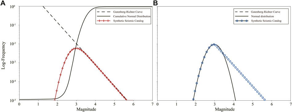
FIGURE 1. Modeling of synthetic seismic catalog. (A) shows the model introduced by Ogata and Katsura (1993). The solid black line and the dashed black line represent the cumulative normal distribution function and the G-R curve, respectively. The red cross is the probability of non-cumulative magnitude in the model. (B) shows the model introduced by Woessner and Wiemer (2005). The solid black line and the dashed black line represent the normal distribution function and the G-R curve, respectively. The blue circle is the probability of non-cumulative magnitude in the model.
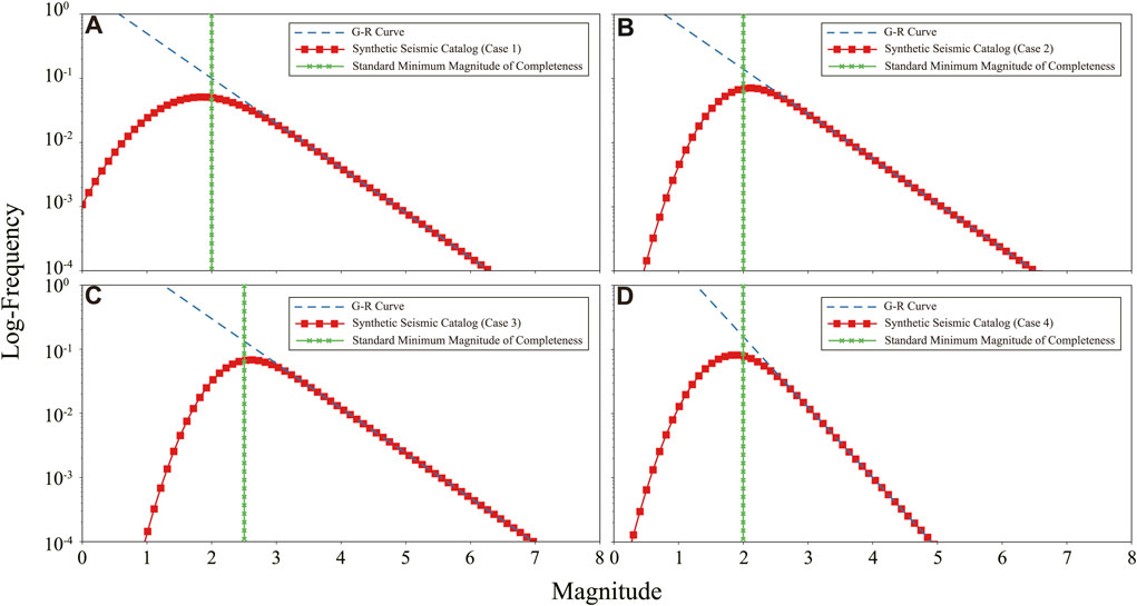
FIGURE 2. The probability density distributions of the four cases. (A–D) are the synthetic seismic catalogs of cases 1–4 from Ogata and Katsura (1993). The greenline is the standard magnitude of Mc, and the blue line is the G–R curve. The red line is the probability of non-cumulative magnitude. The specific parameters are shown in Table 1.
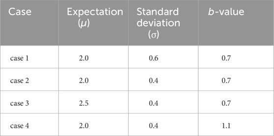
TABLE 1. Model parameters of synthetic seismic catalog.
Figure 3 shows the test results based on case 1 (Mc=2.0; b=0.7). We use the nonlinear least squares method to fit the test results of Mc (red lines in Figure 3). We consider the method with the smallest discrepancy between the estimated Mc and the predefined Mc to be the preferred method. The results show that the fitting curves of Mc calculated by EMR, MMAXC, GFT, MBASS, MAH, and NDT all exhibit approximately linear trends, suggesting that these methods can provide relatively stable Mc across various sample sizes (Figures 3A–C,F–H). Among these methods, the Mc estimated through MMAXC show the best agreement with the standard Mc (Figure 3B), followed by GFT (Figure 3C). MBASS, MAH, and NDT tend to overestimate Mc (Figures 3F–H), while EMR tends to underestimate Mc and displays greater fluctuations (Figure 3A).
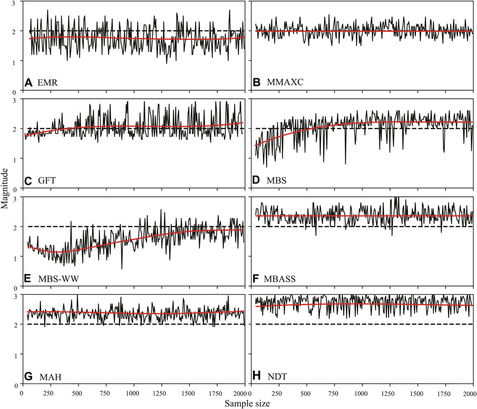
FIGURE 3. Mc as a function of sample size. (A–H) show the Mc estimated by EMR, MMAXC, GFT (90%), MBS, MBS-WW, MBASS, MAH, and NDT in case 1 from Ogata and Katsura (1993), respectively. Black dotted line is the standard magnitude of Mc, and black curve shows the estimated Mc. Red line is the fitting curve of Mc.
In contrast, the fitting curves of Mc calculated by MBS, and MBS-WW exhibit pronounced fluctuations, indicating sensitivity to variations in sample size (Figures 3C–E). These two methods demonstrate an upward trend in Mc as sample size increases, with MBS-WW generally underestimating (Figure 3E), and MBS underestimating in small samples while overestimating in larger samples (Figures 3C,D).
In other cases, methods such as EMR (Supplementary Figure S2A), MBASS (Supplementary Figure S6F), NDT (Supplementary Figure S8H) may have also shown outstanding performance, while GFT may exhibit significant fluctuations. However, observing the test results of all cases (Supplementary Figure S2–S8), MMAXC consistently shows the most stability and is closest to the standard Mc in any cases. In addition, the Mc test results of two different synthetic seismic catalogs are basically consistent. Thus, in this study, we use the MMAXC to calculate Mc.
It is important to emphasize that the testing of Mc methods in this paper is specifically based on the synthetic seismic catalogs. For actual seismic catalogs, the test results of Mc may partially lose effectiveness (actual seismic catalogs are often incomplete). However, the robustness of these methods across various samples holds practical significance as concluded in this paper.
2.3 Methods of b-value estimation
The b-value is an important parameter in seismic hazards analysis (Parsons, 2007; Nanjo and Yoshida, 2018; Gulia and Wiemer, 2019; van der Elst, 2021; Gao et al., 2022). However, its computation is susceptible to various factors, casting doubt on the accuracy of the b-value (especially when seismic catalogs are incomplete or the network for monitor earthquakes is severely disturbed). Alternative and validation methods for the b-value have been proposed (Guttorp, 1987; Parsons, 2007; Telesca et al., 2013; Jiang et al., 2021; Lombardi, 2021; van der Elst, 2021; Li et al., 2023), such as the maximum likelihood method (Aki, 1965), the least square method (Guttorp, 1987), K-S slop (Telesca et al., 2013; Li et al., 2023), and the B-Positive method (van der Elst, 2021). In most cases, the maximum likelihood method derived by Aki (1965) is still the preferred method:
where,
Employing linear least squares regression (LSR) on FMD to determine the b-value is also a straightforward and efficient method (Sandri and Marzocchi, 2007):
where,
The B-Positive is based on the positive-only subset of the differences in magnitude between successive earthquakes, which are described by a double-exponential (Laplace) distribution with the same b-value as the magnitude distribution itself (van der Elst, 2021):
where,
The K-M slope (KMS) obtained from the visibility graph analysis measures the topological connectivity of an event (with magnitude M) to other events (Telesca et al., 2013). The VGA method analyzes the topology of a time series (Li et al., 2023):
where,
The uncertainty of the b-value used in this study is proposed by Shi and Bolt (1982):
where,
2.4 b-value tests based on the simulated seismic catalog by ETAS
Since different estimation methods may lead to different estimations of the b-value, this study conducted a brief examination of these four methods. The method of using synthetic seismic catalog (Ogata and Katsura, 1993; Woessner and Wiemer, 2005) generates a catalog based on preset Mc and b-value, which is the distribution of magnitude-frequency and cannot change with the variation of time and space. However, when it comes to the spatial-temporal variation of b-value, a catalog that can change with time and space is required. The premise of generating such a catalog is to first establish a spatial-temporal point process model of theoretical seismic activity in the corresponding area. Numerous spatial-temporal point process models have been developed to analyze aftershock sequences (Ogata, 1988, 1998; Kagan, 1991; Zhuang et al., 2002; Console et al., 2003; Ogata and Zhuang, 2006). Notably, Ogata (1998) expanded the Epidemic Type Aftershock Sequence (ETAS) model into various spatial-temporal models, drawing upon empirical studies of spatial aftershock clustering and incorporating certain speculative assumptions. This model algorithm measures the goodness of fit using Akaike’s Information Criterion (AIC) (Akaike, 1974) and can simulate a high-quality dataset similar to instrumental seismic catalog (Ogata, 1998).
This study extracts partial segments of the instrumental seismic catalog within the eastern Tibetan Plateau (from January 2013 to January 2015) for predicting the ETAS model of the region. We utilized the code developed by Ogata (1998) to invert the parameters of the ETAS model for the eastern Tibetan Plateau. Because the spatial distribution of earthquakes within the area is uneven, in order to improve the prediction accuracy of the ETAS model, we conducted a spatial inversion of five parameters in the ETAS model. We applied the best parameters (Supplementary Figure S9) to the conditional intensity for the occurrence time of point process in the ETAS model and generated 100 sets of simulated catalogs with the best parameters, from which we selected the best simulated catalog (Supplementary Figure S10). A comparison between the optimal simulated catalog and the instrumental catalog reveals that several major earthquakes in the instrumental catalog are effectively reproduced (Supplementary Figure S10). The b-value of the overall catalog simulated by the ETAS model is 0.77 ± 0.03 (Supplementary Figure S11).
We employed four methods to compute the b-value in the simulated catalog (Supplementary Figure S10). The results indicate that the b-value estimated by LSR fluctuate significantly at the given time windows (Red dotted box in Figure 4), whereas the b-value for B-Positive and KMS only show significant fluctuations before and after major earthquakes. In contrast, the b-value estimated by MLE is relatively stable with small fluctuation (Figure 4).
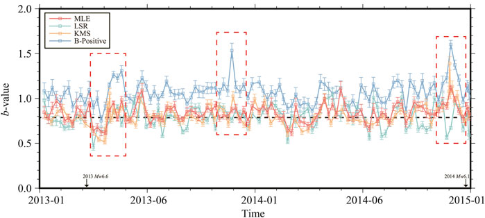
FIGURE 4. The b-value as a function of time in the simulation catalog. Red, green, yellow, and blue lines represent the b-value calculated by MLE, LSR, KMS, and B-Positive, respectively. Red dotted box is the specific comparison window.
In addition, the estimated b-value by B-Positive is generally higher than the regional average b-value (0.77). LSR is on the lower side, while MLE and KMS remain stable around the regional average b-value fluctuation (Figure 4). Considering the algorithm’s requirement for both stability and accuracy, MLE satisfies these characteristics. Therefore, in the following study, we choose MLE to calculate the b-value.
3 Spatial-temporal distribution of b-value in the eastern Tibetan Plateau
The eastern Tibetan Plateau is a transitional zone between the Tibetan Plateau and the South China block. Following the collision of the Indian plate to Eurasia in early Tertiary, the eastern Tibetan Plateau has undergone intense tectonic movements and frequent seismic activity (Avouac and Tapponnier, 1993; Tapponnier et al., 2001; Royden et al., 2008; Deng et al., 2019) (Figure 5). In recent years, the eastern Tibetan Plateau has been intensely seismically active, generating the 2008 Mw 7.9 Wenchuan earthquake, 2013 Mw 6.6 Lushan, 2014 Mw 6.1 Kangding, 2017 Mw 6.5 Jiuzhaigou and 2022 Mw 6.6 Luding (Figure 5). The frequent seismicity in the eastern Tibetan Plateau has aroused great concern to geoscientists (Yi et al., 2008; Wang et al., 2012; Liu et al., 2015; Jiang and Feng, 2021; Gao et al., 2022; Jiang et al., 2022).
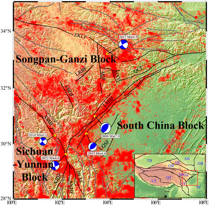
FIGURE 5. Tectonic background of the eastern Tibetan Plateau. Red circles show the location of earthquakes from 1970 to 2023. Seismic data are from the China Earthquake Network Center. Blue beach balls are the focal mechanism solutions of earthquake from GCMT (http://www.globalcmt.org). LMSF: Longmen Shan fault; XSHF: Xianshuihe fault; EKLF: East Kunlun fault; XJHF: Xiaojinhe fault; DLSF: Daliang Shan fault; ANHF: Anninghe fault; QCF: Qingchuan fault; HYF: Huya fault; MJF: Minjiang fault; FBHF: Fubianhe fault; LQSF: Longquan Shan fault; LRBF: Longriba fault. The lower right corner diagram shows a larger area tectonic map, where QT: Qiangtang block, LS: Lhasa block, TB: Tarim Basin, QB: Qaidam Basin, QL: Qilian block, SPGZ: Songpan-Ganzi block, AB: Alashan block, OB: Ordos block, SC: South China block, SY: Sichuan-Yunnan block.
3.1 Instrumental seismic catalog in the eastern Tibetan Plateau
The instrumental seismic catalog is the fundamental dataset for seismic prediction and statistical analysis (Li et al., 2015). In this study, we acquired a seismic catalog from the China Earthquake Network Center for the study area spanning from January 1970 to August 2023 (longitude: 100ºE-108ºE, latitude: 28ºN-35ºN) (Figure 5). The catalog comprises a total of 841,095 data entries, with earthquake magnitudes ranging from 0.1 to 8.1. The statistical results of cumulative earthquake frequency (red line in Figure 6A) indicate a gradual rise in the number of earthquakes starting from 2000, with a sharp increase after 2008. We’ve tallied up the number of earthquakes each month in the instrumental seismic catalog (Figure 6B), and the results further emphasize a notable increase in the number of earthquakes from 2000. This coincides with the second upgrade of the China Earthquake Network from 2000 to 2008 (Zheng et al., 2009), which significantly improved the network’s ability to monitor earthquakes and explains the rapid growth in the cumulative count in the catalog. To ensure the accuracy and reliability of the seismic catalog, we used the time range from 2000 to 2023.
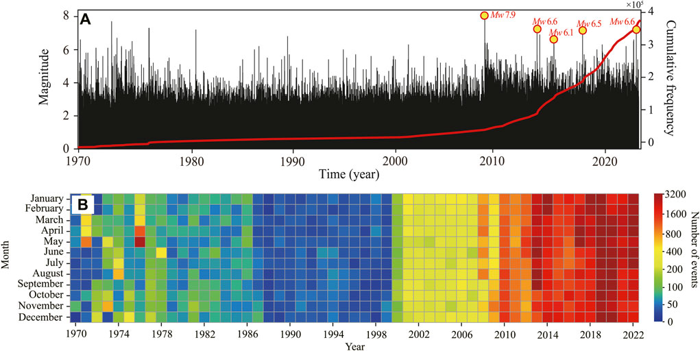
FIGURE 6. Statistical analysis of the instrumental seismic catalog. (A) shows the magnitude-time distribution, the red line represents the cumulative earthquake frequency. (B) is the monthly statistics of the seismic catalog.
3.2 The temporal evolution of b-value in the eastern Tibetan Plateau
In order to observe the temporal evolution of b-value before and after major earthquakes in the eastern Tibetan Plateau, we computed the b-value for the region spanning from 2000 to 2023. We set the time window of 2-month for the calculations, with each window employing the MMAXC to calculate Mc and MLE to calculate the b-value. Commonly, it is accepted that the clustering of aftershocks obscures the statistical features of the mainshocks as an independent event (Gardner and Knopoff, 1974; Taroni and Akinci, 2021). To eliminate this effect, we use Reasenberg (1985) method to remove the aftershock sequence from major earthquakes. Reasenberg (1985) models the earthquake process as a five-dimensional point process and uses the second-order moment to describe the distribution of event pairs in the seismic catalog, which can more accurately determine the clustering of aftershocks.
The results indicate that from 2000 to 2008, the b-value exhibited significant fluctuations (Figure 7). However, after 2008, the b-value remained relatively stable, with only slight fluctuations during earthquakes. This may be related to discrepancies in the monitoring capabilities of the network during different time periods, leading to variations in the completeness of the seismic catalog. Before the five major earthquakes in the study area, the b-value all showed varying degrees of decline (the maximum decrease of b-value before each earthquake, 0.57 in the 3.5 years before the 2008 Wenchuan, 0.14 in the 21 months before the 2013 Lushan, 0.17 in the 9 months before the 2014 Kangding, 0.15 in the 3 months before the 2017 Jiuzhaigou, and 0.09 in the 6 months before the 2022 Luding, for example, the green dotted box in Figure 7), reaching their lowest point at the moment of the earthquake (2008 Wenchuan: 0.58; 2013 Lushan: 0.79; 2014 Kangding: 0.77; 2017 Jiuzhaigou: 0.80; 2022 Luding: 0.83). After the earthquake, the b-value gradually returned to its initial level. Among them, the temporal variation of b-value before and after the 2008 Wenchuan earthquake is the most obvious and lasts longer compared to the subsequent four major earthquakes.
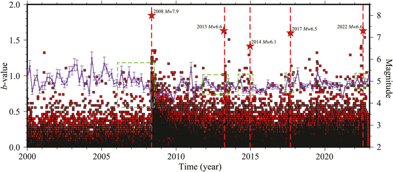
FIGURE 7. The temporal evolution of b-value. The purple line and error bars represent the b-value and the uncertainty of b-value; the red dashed line indicates the moments of the earthquake; the red square represents the earthquake; the red five-pointed star represents the five major earthquakes in the region. The green dashed box represents the potential drop phase of b-value for each earthquake.
Among the five major earthquakes, we observed a consistent trend in the temporal evolution of b-value: b-value decreases before earthquakes, while the value increases after earthquakes. This trend aligns with findings in rock mechanics and acoustic emissions research, where the b-value decreases as rocks approach failure and increases as the rocks undergo healing (Scholz, 1968; Zhao et al., 2019; Dong et al., 2022).
3.3 The spatial distribution of b-value in the eastern Tibetan Plateau
To analyze the spatial-temporal evolution of b-value before and after major earthquakes in the eastern Tibetan Plateau. We have categorized five distinct time periods based on the sequence of earthquake: T1 (2000.01.01-2008.05.11): Before the 2008 Wenchuan earthquake; T2 (2008.05.12-2013.04.19): After the 2008 Wenchuan earthquake and before the 2013 Lushan earthquake; T3 (2013.04.20-2014.11.24): After the 2013 Lushan earthquake and before the 2014 Kangding earthquake; T4 (2014.11.25-2017.08.07): After the 2014 Kangding earthquake and before the 2017 Jiuzhaigou earthquake; T5 (2017.08.08-2022.09.05): After the 2017 Jiuzhaigou earthquake and before the 2022 Luding earthquake. We divide the area into 0.1° × 0.1° grids (with a unit area of 10 km2) and use a dynamic search radius to search for events in each grid: each grid initially searched within a 20 km radius. If the number of events did not meet the minimum requirement (N≥50), we increased the search radius by 10 km and repeated the process until the condition was met (Rmax=60 km). Additionally, we require a minimum magnitude difference of at least 2.5 between events within a grid. If these conditions are not satisfied, Mc and b-value is not calculated within this grid.
The results of Mc show significant spatial heterogeneity in the eastern Tibetan Plateau during T1 and T2 (Figures 8A,B). However, from T3 to T5, the distribution of Mc is relatively uniform (Figures 8C–E).
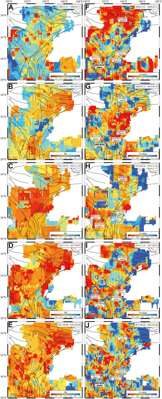
FIGURE 8. The spatial distribution of Mc and b-value. (A–E) show the spatial distribution of Mc from T1 to T5, (F–J) are the spatial distribution of b-value from T1 to T5.
The spatial distribution of b-value indicates significant heterogeneity in the eastern Tibetan Plateau across five time periods (Figures 8F–J). During the T1 period, the middle LMSF, XSHF, and DKLF all fall within a low b-value area compared to their surroundings. Overall, b-value inside SPGZ is higher than those in the surrounding faults (Figure 8F). During the T2 period, the b-value exhibit nearly opposite distribution compared to the T1, with low values concentrated in LMSF, gradually increasing from the center of LMSF outwards (Figure 8G). During the T3 period, the b-value distribution is relatively uniform, with most areas showing a b-value of around 0.9, except for exceptionally low values in the southern XSHF and the northern LQSF (Figure 8H). The spatial distribution pattern of b-value in T4 and T5 remains consistent. Both the eastern DKLF in T4 and the southern XSHF in T5 are situated in areas characterized by very low b-value (Figure 8J).
Overall, with the successive occurrence of earthquakes, the spatial distribution of the b-value in the region will also change accordingly. The most significant change in spatial distribution of b-value occurs during the transition from T1 to T2, where the distribution becomes nearly opposite. It is noteworthy that the epicenters of the five major earthquakes in the region were all situated in the low b-value area relative to the surrounding areas prior to the earthquakes.
3.4 Seismic hazards combined maximum shear strain rate with b-value in the eastern Tibetan Plateau
The spatial distribution of b-value may reflect the background stress accumulation of different regions (Amitrano, 2003; Dong et al., 2022; Li et al., 2022; Mogi, 1967; Scholz, 1968, Scholz, 2015; Schorlemmer et al., 2005; W. Goebel et al., 2013), while the spatial distribution of maximum shear strain rate derived from GPS observations may indicate the present-day stress accumulation rates (assuming the crust material is elastic, the stress rates and strain rates have a linear relationship). We divide the region into calculation points of 0.1°×0.1° and use the velocity interpolation for strain rate program developed by Shen et al. (2015) to calculate the maximum shear strain rate at each point. We use tensor curvature spline interpolation to interpolate the study area. The GPS data used in the calculation of the maximum shear strain rate comes from the processed Chinese mainland GPS data from 1991 to 2016 by Wang and Shen (2020). We are attempting to qualitatively identify similarities in regional seismic hazards using two distinct sets of data, with the aim of obtaining more valuable information through this comparison.
The results indicate that the maximum shear strain rate in the SPGZ and the SY are significantly higher than that in the SC, with the highest values located at XSHF-ANHF-ZMHF (Figure 9A). Meanwhile, the spatial distribution of b-value in the eastern Tibetan Plateau has significant heterogeneity, with low b-value mainly concentrated near the fault zone (Figure 9B).
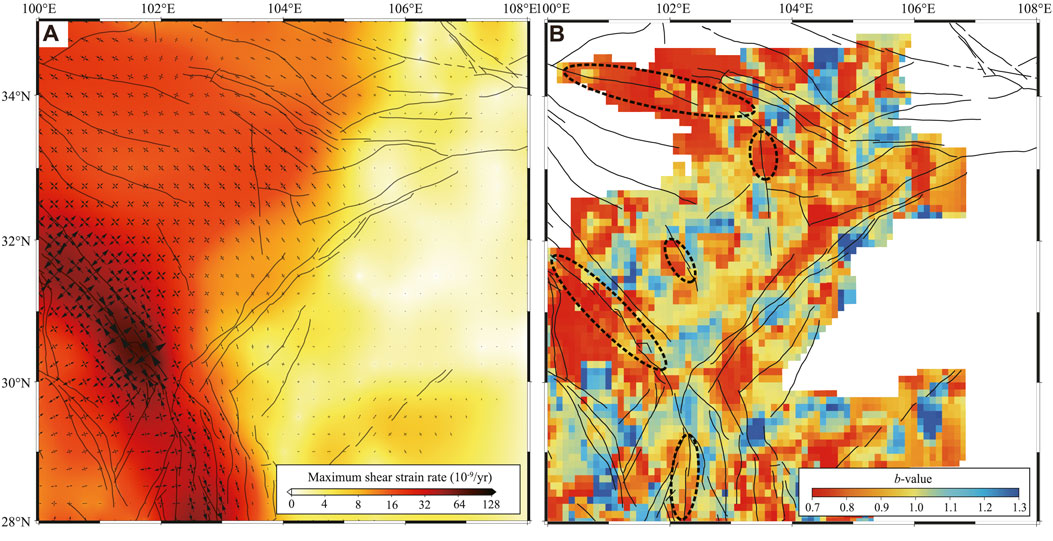
FIGURE 9. Distribution of the maximum shear strain rate (A) and b-value in the eastern Tibetan Plateau (B). The black dashed circles show the regions with both low b-value and high shear strain rate.
The maximum shear strain rate may reflect the accumulation rate of shear strain in a region, while the b-value reflects the accumulation state of background stress in the region. These two have similar physical meanings. By combining areas with high maximum shear strain rate and low b-value, we qualitatively identified five regions with high potential of seismic hazards in the eastern Tibetan Plateau: XSHF (Ganzi-Luhuo-Daofu-Qianning-Kangding segment), DKLF (Maqin-Maqu segment), ANHF, FBHF, and northern MJF.
4 Discussion
The temporal evolution of b-value for the five major earthquakes in the eastern Tibetan Plateau (2008 Mw 7.9 Wenchuan, 2013 Mw 6.6 Lushan, 2014 Mw 6.1 Kangding, 2017 Mw 6.5 Jiuzhaigou and 2022 Mw 6.6 Luding) exhibits a consistent trend (Figure 7): the b-value decreases before the earthquake and rises afterward. This trend might reflect the accumulation and release of stress on the fault. With tectonic loading, stress on the fault continuously increases, while the b-value gradually decreases. When the accumulated stress on faults reaches a critical threshold, earthquakes occurred. After an earthquake occurs, the stress on the fault is released, and the b-value gradually increases. In addition, in the five major earthquakes on the eastern Tibetan Plateau, the decrease and increase trends of the b-value for the 2008 Wenchuan earthquake were the most noticeable (with a decrease of about 0.57) and persistent (∼3.5 years) (Figure 7). In contrast, the b-value for the other four earthquakes showed smaller variations (2013 Lushan: 0.14; 2014 Kangding: 0.17; 2017 Jiuzhaigou: 0.15; 2022 Luding: 0.09) and only lasted for a few months. This seems to be related to the magnitude: the 2008 Wenchuan earthquake had the highest magnitude, while the other four earthquakes had relatively smaller magnitudes. It is important to note that the amplitude of the decrease in b-value may change, as it is related to the uncertainty of the b-value in its temporal evolution (the average uncertainty of b-value within the decrease range of b-value for each earthquake, 2008 Wenchuan: 0.10, 2013 Lushan: 0.06, 2014 Kangding: 0.06, 2017 Jiuzhaigou: 0.08, 2022 Luding: 0.07, as shown in Figure 7). In addition, the data used to calculate the temporal evolution of b-value is the seismic catalog of the entire region in this study, which may lead to the calculation of b-value for specific earthquakes being influenced by events from other areas. Therefore, we calculated the temporal evolution of b-value in small areas around the epicenter of each earthquake (the small area being the aftershock range of each earthquake, assuming that the influence of the earthquake range is consistent with the aftershock range. Red circle in Supplementary Figure S12). The results also show that the b-value have different degrees of decrease before each earthquake (the maximum decrease of b-value before each earthquake, 0.78 in the 15 months before the 2008 Wenchuan, 0.37 in the 1 year before the 2013 Lushan, 0.18 in the 6 months before the 2014 Kangding, 0.53 in the 3.5 years before the 2017 Jiuzhaigou, and 0.42 in the 1 year before the 2022 Luding, for example, the green dotted box in Supplementary Figure S13), decreasing trend of b-value calculated for the entire region (Figure 7). However, the amplitude of the decrease in b-value calculated for small areas is greater than that calculated for the entire region. This suggests that although the temporal evolution of the b-value for the entire region includes some characteristics of the b-value for small areas, the b-value calculated for small areas seem to better reflect the specific changes in b-value for that particular area.
The spatial distribution of b-value before the five earthquakes in the eastern Tibetan Plateau reveals a consistent pattern (Figure 8): the epicenters of earthquakes tend to be situated in areas with lower b-value compared to the surrounding regions before the earthquakes. Given the inverse correlation between b-value and stress (Amitrano, 2003; Dong et al., 2022; Li et al., 2022; Mogi, 1967; Scholz, 1968, Scholz, 2015; Schorlemmer et al., 2005; W. Goebel et al., 2013), this may indicate that there is a high stress accumulation near the epicenters before each of the five earthquakes. This is consistent with the study finding that regional seismic activity is mainly concentrated in spatial locations with lower b-value (Nanjo et al., 2012; Zhang and Zhou, 2016; Nanjo and Yoshida, 2018; Jiang and Feng, 2021; Jiang et al., 2022; Sun et al., 2023). Whether an earthquake occurs mainly depends on the background stress that has already accumulated on the fault (Luo and Liu, 2018; Sun et al., 2020; Sun et al., 2023). The characteristic of b-value allows us to use it to understand the characteristics of regional seismic activity distribution (Smith, 1981; Nanjo et al., 2012; Wang et al., 2012; Liu et al., 2015; Gao et al., 2022) and further analyze seismic hazard areas.
The spatial distribution of b-value may effectively reflect the differences in local stress accumulation, enabling us to delineate potential seismic hazards on faults (Liu et al., 2015; Liu and Pei, 2017; Gao et al., 2022). Furthermore, the maximum shear strain rate serves as an indicator of shear stress accumulation rates in a region (assuming the crust material is elastic, the stress rates and strain rates have a linear relationship), and can also determine the seismic hazards. We note that the accumulation rate of stress also depends on the frictional characteristics of the fault (Ikari et al., 2011). This study did not consider the impact of this factor. We combine areas with high shear strain rate and low b-value, and qualitatively identify five regions with high potential of seismic hazards in the eastern Tibetan Plateau: XSHF (Ganzi-Luhuo-Daofu-Qianning-Kangding segment), DKLF (Maqin-Maqu segment), ANHF, FBHF, and northern MJF (the black dotted circle in Figure 9B). Paleo-earthquake researches also indicate that there are seismic gaps in the above five regions: Daofu-Qianning segment on XSHF (Han and Huang, 1983; Yi et al., 2008), Mianning-Xichang segment on ANHF (Wen et al., 2008), Maqin-Maqu segment on DKLF (Li et al., 2019), northern FBHF (Liu et al., 2007), and northern MJF (Li et al., 2018). Overall, we should pay attention to five high potential seismic hazard zones delineated by combining the results of b-value and the maximum shear strain rate, which are also identified as seismic gaps through paleo-earthquake studies (Han and Huang, 1983; Liu et al., 2007; Wen et al., 2008; Yi et al., 2008; Chen et al., 2013; Xu et al., 2013; Pei et al., 2014; Li et al., 2018; Li et al., 2019). We note that there is still a seismic gap on the southern LMSF. This seismic gap exhibits a low b-value and a low shear strain rate, which may indicate that although the present-day tectonic loading rates within the seismic gap is slow, it has accumulated a significant amount of stress over long-term tectonic loading. Furthermore, there has not been a major earthquake for a century (Chen and Hsu, 2013), which means that the stress accumulated in this seismic gap has not been released yet. Therefore, the seismic gap in the southern LMSF should also be a concern for future seismic hazards.
Although it is generally believed that the spatial-temporal changes of the b-value are consistent before and after an earthquake (b-value decrease before, and increase after), some studies suggest that the changes in time and space may be influenced by artificial factors such as incomplete catalogs or calculation methods (Jackson and Kagan, 1999; Del Pezzo, 2003; Amorèse et al., 2010). In addition, an increase in the b-value before many seismic events has been observed (Smith, 1981; Nuannin, 2006; Nuannin et al., 2012; El-Isa, 2013), which is a crucial factor in the misjudgment of FTLS (Gulia and Wiemer, 2019). The research findings in this paper support the common trend of decreasing b-value before major earthquakes within the eastern Tibetan Plateau.
The calculation of the spatial-temporal distribution of b-value can be influenced by various factors. In addition to the factors already tested in the study, we have also explored other factors. The length of time window will affect the FMD within a window, which in turn affects the calculation of b-value. Therefore, we use time windows of 2, 4, 6, and 8 months to calculate the b-value (Figure 10). The results indicate that the b-value shows a consistent trend within different time windows, meaning that the b-value decreases before the earthquake and increases after it. As the time window increases, the change in b-value becomes more stable. When the time window decreases, the fluctuation of b-value increases. However, no matter the size of the time window, the temporal evolution trend of b-value will not change. Therefore, choosing a smaller time window can be used to observe the short-term evolution of b-value, while a larger time window is used for the long term.
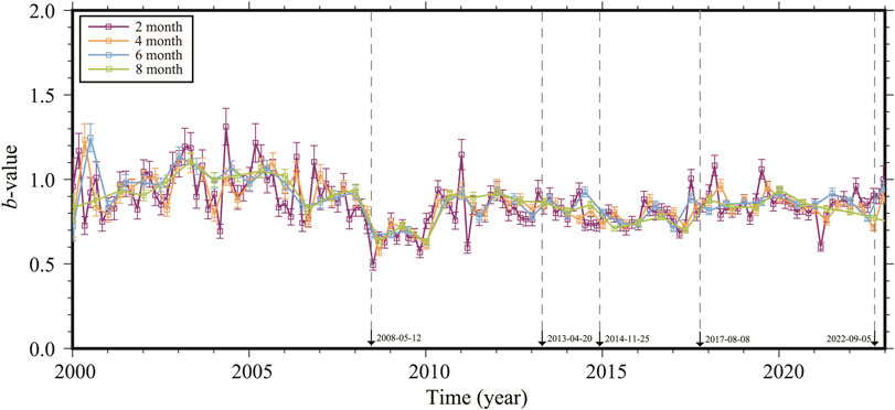
FIGURE 10. The temporal evolution of b-value under different time windows. The purple, yellow, blue, and green lines are the temporal evolutions of b-value in the time window of 2, 4, 6 and 8 months respectively.
There are typically two options for calculating the temporal evolution of b-value: time windows or sample windows. To examine the impact of these methods for b-value, we also calculated the temporal evolution of b-value using sample windows of 400, 600 and 800. The results reveal that the temporal trend of b-value remains consistent across different sample windows (Figure 11) and aligns with the outcomes obtained using time windows (Figure 10). However, since 2008, the number of calculation points of b-value has significantly increased, and the fluctuation of b-value are greater. This is related to the significant increase in cumulative earthquake frequency in the seismic catalog after 2008. Therefore, the sampling window method is not suitable for cases with significant changes in cumulative earthquake frequency. But whether you choose a time window or a sample window, both methods show a consistent overall trend in b-value.
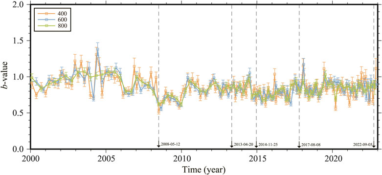
FIGURE 11. The temporal evolution of b-value under different sample windows. The yellow, blue and green lines are the temporal evolutions of b-value in the sample window of 400, 600 and 800 respectively.
We assessed the impact of different maximum search radius (30, 60, and 90 km) on the spatial distribution of b-value during the T1 period. The results indicate that as the search radius increases, the spatial distribution of b-value becomes more uniform while maintaining a consistent spatial pattern (Figure 12).
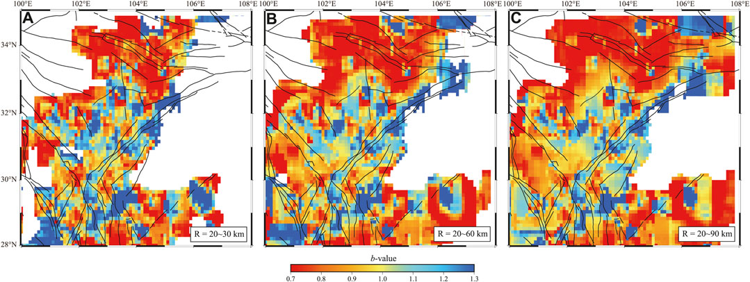
FIGURE 12. Spatial distribution of b-value under different maximum search radius. (A–C) are the spatial distribution of b-value when the maximum search radius are 30, 60 and 90 km respectively.
We also investigated the influence of varying number requirements (30, 50, and 80) on the spatial distribution of b-value. The results reveal that with higher number requirements, the distribution of b-value becomes more uniform while still maintaining a consistent spatial pattern (Figure 13).
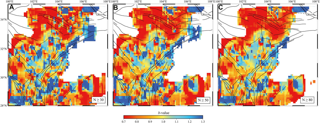
FIGURE 13. Spatial distribution of b-value under different number requirements. (A–C) are the spatial distribution of b-value when the number requirements are 30, 50 and 80 respectively.
Overall, while several factors may impact the results of b-value, they will not change the overall temporal trend and spatial distribution of b-value (Figure 10, Figure 11, Figure 12; Figure 13). The results of this study will remain consistent with different parameters. The reliability of b-value primarily depends on the completeness and accuracy of seismic catalog. However, historical seismic catalog is often incomplete, and modern seismic catalog has a short time span. Thus, enhancing the completeness of seismic catalog is fundamental for the study of b-value.
5 Conclusion
The spatial-temporal evolution of b-value is one of the most important indexes for seismological research and seismic hazards assessment, while the accuracy of the b-value largely depended on the completeness of seismic catalog and methods of calculating the b-value. This study tested eight methods in estimating the minimum magnitude of completeness and four methods in estimating b-value based on synthetic seismic catalogs. Based on the test results, we choose the optimal method in estimating Mc and b-value suitable for this study. We then calculate Mc and b-value in the eastern Tibetan Plateau.
1. The test results for eight methods in estimating Mc indicate that MMAXC consistently exhibits the highest stability and accuracy across different sample sizes and cases.
2. The temporal evolution of b-value of the five major earthquakes in the eastern Tibetan Plateau shows a consistent trend: the b-value decreases before earthquakes (the maximum decrease in b-value for each earthquake, 2008 Wenchuan: 0.57, 2013 Lushan: 0.14, 2014 Kangding: 0.17, 2017 Jiuzhaigou: 0.15, 2022 Luding: 0.09), and increases after earthquakes (rising to around 1.0). This may correspond to the two processes of stress accumulation and release during earthquakes.
3. The spatial distribution of b-value of the five major earthquakes in the eastern Tibetan Plateau shows that the epicenters of the earthquakes were located in the regions with lower b-value before each earthquake. This may indicate that there was a significant stress accumulation near the epicenters before all five earthquakes. Therefore, the b-value may be used to identify high-stress areas, further determining seismic hazard regions.
4. There are five regions with both lower b-value and higher maximum shear strain rate in the eastern Tibetan Plateau: Ganzi-Luhuo-Daofu-Qianning-Kangding, Maqin-Maqu, ANHF, FBHF, and northern MJF, which may indicate high-stress accumulation and high seismic hazards in the future.
Data availability statement
The original contributions presented in the study are included in the article/Supplementary Material, further inquiries can be directed to the corresponding authors.
Author contributions
WG: Conceptualization, Data curation, Formal Analysis, Investigation, Methodology, Software, Validation, Visualization, Writing–original draft, Writing–review and editing. HC: Methodology, Project administration, Supervision, Writing–review and editing. YG: Data curation, Investigation, Validation, Writing–review and editing. QL: Data curation, Formal Analysis, Project administration, Supervision, Writing–review and editing. YS: Conceptualization, Formal Analysis, Funding acquisition, Investigation, Methodology, Project administration, Resources, Supervision, Validation, Visualization, Writing–review and editing.
Funding
The author(s) declare financial support was received for the research, authorship, and/or publication of this article. This research is supported by Natural Science Foundation of Fujian Province (2022J05039), National Natural Science Foundation of China (42104094), Open Foundation of the United Laboratory of Numerical Earthquake Forecasting (2021LNEF03), and Startup Foundation of Wuyi University’s Talents Introduction Research Project (YJ202218).
Acknowledgments
The author appreciates the comments from editor Paolo Capuano and three reviewers, which helped improve and clarify the article.
Conflict of interest
The authors declare that the research was conducted in the absence of any commercial or financial relationships that could be construed as a potential conflict of interest.
Publisher’s note
All claims expressed in this article are solely those of the authors and do not necessarily represent those of their affiliated organizations, or those of the publisher, the editors and the reviewers. Any product that may be evaluated in this article, or claim that may be made by its manufacturer, is not guaranteed or endorsed by the publisher.
Supplementary material
The Supplementary Material for this article can be found online at: https://www.frontiersin.org/articles/10.3389/feart.2024.1335938/full#supplementary-material
References
Akaike, H. (1974). A new look at the statistical model identification. IEEE Trans. automatic control 19 (6), 215–222. doi:10.1007/978-1-4612-1694-0_16
Aki, K. (1965). Maximum likelihood estimate of b in the formula logN=a-bM and its confidence limits. Bull. Earthq. Res. Inst. Univ. Tokyo 43, 237–239.
Amitrano, D. (2003). Brittle-ductile transition and associated seismicity: experimental and numerical studies and relationship with the b value. J. Geophys. Res. Solid Earth 108 (B1). doi:10.1029/2001JB000680
Amorèse, D. (2007). Applying a change-point detection method on frequency-magnitude distributions. Bull. Seismol. Soc. Am. 97 (5), 1742–1749. doi:10.1785/0120060181
Amorèse, D., Grasso, J. R., and Rydelek, P. A. (2010). On varying b-values with depth: results from computer-intensive tests for Southern California. Geophys. J. Int. 180 (1), 347–360. doi:10.1111/j.1365-246X.2009.04414.x
Avouac, J. P., and Tapponnier, P. (1993). Kinematic model of active deformation in central Asia. Geophys. Res. Lett. 20 (10), 895–898. doi:10.1029/93GL00128
Cao, A., and Gao, S. S. (2002). Temporal variation of seismic b-values beneath northeastern Japan island arc. Geophys. Res. Lett. 29 (9), 1334. doi:10.1029/2001GL013775
Chen, W., and Hsu, L. (2013). Historic seismicity near the source zone of the great 2008 Wenchuan earthquake: implications for seismic hazards. Tectonophysics 584, 114–118. doi:10.1016/j.tecto.2012.08.035
Chen, Y., Yang, Z., Zhang, Y., and Liu, C. (2013). From the Wenchuan earthquake to the Lushan earthquake. Sci. China Earth Sci. 43 (6), 1064–1072. doi:10.1360/zd-2013-43-6-1064
Clauset, A., Shalizi, C. R., and Newman, M. E. (2009). Power-law distributions in empirical data. SIAM Rev. 51 (4), 661–703. doi:10.1137/070710111
Console, R., Murru, M., and Lombardi, A. M. (2003). Refining earthquake clustering models. J. Geophys. Res. Solid Earth 108 (B10). doi:10.1029/2002jb002130
Del Pezzo, E. (2003). Discrimination of earthquakes and underwater explosions using neural networks. Bull. Seismol. Soc. Am. 93 (1), 215–223. doi:10.1785/0120020005
Deng, D., Wang, C., and Peng, P. (2019). Basic characteristics and evolution of geological structures in the eastern margin of the Qinghai-Tibet plateau. Earth Sci. Res. J. 23 (4), 283–291. doi:10.15446/esrj.v23n4.84000
Dong, L., Zhang, L., Liu, H., Du, K., and Liu, X. (2022). Acoustic emission b value characteristics of granite under true triaxial stress. Mathematics 10 (3), 451. doi:10.3390/math10030451
El-Isa, Z. H. (2013). Continuous-cyclic variations in the b-value of the earthquake frequency-magnitude distribution. Earthq. Sci. 26 (5), 301–320. doi:10.1007/s11589-013-0037-9
El-Isa, Z. H., and Eaton, D. W. (2014). Spatiotemporal variations in the b-value of earthquake magnitude-frequency distributions: classification and causes. Tectonophysics 615-616, 1–11. doi:10.1016/j.tecto.2013.12.001
Gao, Y., Luo, G., and Sun, Y. (2020). Seismicity, fault slip rates, and fault interactions in a fault system. J. Geophys. Res. Solid Earth 125 (2), e2019JB017379. doi:10.1029/2019JB017379
Gao, Y., Sun, Y., and Luo, G. (2022). Temporal and spatial evolution characteristics of b value and stress field in Taiwan before and after the 1999 Chi-Chi Earthquake. Chin. J. Geophys. (in Chinese) 65 (6), 2137–2152. doi:10.6038/cjg2022P0106
Gardner, J. K., and Knopoff, L. (1974). Is the sequence of earthquakes in Southern California, with aftershocks removed, Poissonian? Bulletin of the Seismological Society of America 64 (5), 1363–1367. doi:10.1785/bssa0640051363
Gerstenberger, M., Wiemer, S., and Giardini, D. (2001). A systematic test of the hypothesis that the b value varies with depth in California. Geophysical Research Letters 28 (1), 57–60. doi:10.1029/2000gl012026
Godano, C. (2017). A new method for the estimation of the completeness magnitude. Physics of the Earth and Planetary Interiors 263, 7–11. doi:10.1016/j.pepi.2016.12.003
Goebel, W., Schorlemmer, D., Becker, T. W., Dresen, G., and Sammis, C. G. (2013). Acoustic emissions document stress changes over many seismic cycles in stick-slip experiments. Geophysical Research Letters 40 (10), 2049–2054. doi:10.1002/grl.50507
Gomberg, J. (1991). Seismicity and detection/location threshold in the southern Great Basin seismic network. Journal of Geophysical Research Solid Earth 96 (B10), 16401–16414. doi:10.1029/91JB01593
Gulia, L., and Wiemer, S. (2019). Real-time discrimination of earthquake foreshocks and aftershocks. Nature 574 (7777), 193–199. doi:10.1038/s41586-019-1606-4
Gutenberg, B., and Richter, C. F. (1944). Frequency of earthquakes in California. Bulletin of the Seismological Society of America 34 (4), 185–188. doi:10.1785/BSSA0340040185
Guttorp, P. (1987). On least-squares estimation of b values. Bulletin of the Seismological Society of America 77 (6), 2115–2124. doi:10.1785/BSSA0770062115
Han, W., and Huang, S. (1983). A seismic gap on the Xianshuihe fault, Sichuan province. Acta Seismologica Sinica 5 (3).
Huang, Y., Zhou, S., and Zhuang, J. (2016). Numerical tests on catalog-based methods to estimate magnitude of completeness. Chinese Journal of Geophysics (in Chinese) 59 (4), 1350–1358. doi:10.6038/cjg20160416
Ikari, M. J., Marone, C., and Saffer, D. M. (2011). On the relation between fault strength and frictional stability. Geology 39 (1), 83–86. doi:10.1130/g31416.1
Iwata, T. (2008). Low detection capability of global earthquakes after the occurrence of large earthquakes: investigation of the Harvard CMT catalogue. Geophysical Journal International 174 (3), 849–856. doi:10.1111/j.1365-246x.2008.03864.x
Jackson, D. D., and Kagan, Y. Y. (1999). Testable earthquake forecasts for 1999. Seismological Research Letters 70 (4), 393–403. doi:10.1785/gssrl.70.4.393
Jiang, C., Jiang, C., Yin, F., Zhang, Y., Bi, J., Long, F., et al. (2021). A new method for calculating b-value of time sequence based on data-driven (TbDD): a case study of the 2021 Yangbi Ms6.4 earthquake sequence in Yunnan. Chinese Journal of Geophysics (in Chinese) 64 (09), 3126–3134. doi:10.6038/cig2021P0385
Jiang, J., and Feng, J. (2021). Stress state and b-value anomalies before the Jiuzhaigou Ms7.0 earthquake in 2017. China Earthquake Engineering Journal 43 (3), 575–582. doi:10.3969/j.issn.1000-0844.2021.03.575
Jiang, Y., Liu, Z., Zhang, X., Zhang, L., and Wei, J. (2022). Variation features of b-value before and after the 2021 Maduo Mw 7.4 earthquake. Geomatics and Information Science of Wuhan University 47 (6), 907–915. doi:10.13203/j.whugis20220071
Kagan, Y. Y. (1991). Likelihood analysis of earthquake catalogues. Geophysical Journal International 106 (1), 135–148. doi:10.1111/j.1365-246x.1991.tb04607.x
Kværna, T., Ringdal, F., Schweitzer, J., and Taylor, L. (2002). Optimized seismic threshold monitoring-part 1: regional processing. Pure and Applied Geophysics 159, 969–987. doi:10.1007/s00024-002-8668-0
Li, B., Ding, Q., Xu, N., Dai, F., Xu, Y., and Qu, H. (2022). Characteristics of microseismic b-value associated with rock mass large deformation in underground powerhouse caverns at different stress levels. Journal of Central South University 29 (2), 693–711. doi:10.1007/s11771-022-4946-4
Li, F., Liu, H., Jia, Q., Xu, X., Zhang, X., and Gong, F. (2018). Holocene active characteristics of the northern segment of the Minjiang Fault in the eastern margin of the Tibetan Plateau. Seismology and Geology 40 (01), 97–106. doi:10.3969/j.issn.0253-4967.2018.01.008
Li, H., Deng, Z., Xing, C., Yan, X., Ma, X., and Jiang, H. (2015). Progress in research on synthetic earthquake catalogues. Progress in Geophysics (in Chinese) 30 (5), 1995–2006. doi:10.6038/pg20150503
Li, J., Zhang, J., and Cai, Y. (2019). Investigation of historical earthquakes, paleo-earthquakes and seismic gap in the eastern Kunlun fault zone. Earthquake 37 (1), 103–111.
Li, L., Luo, G., and Liu, M. (2023). The K-M slope: a potential supplement for b-value. Seismological Research Letters. doi:10.1785/0220220268
Lin, J., Sibuet, J. C., Lee, C., Hsu, S., and Klingelhoefer, F. (2007). Spatial variations in the frequency-magnitude distribution of earthquakes in the southwestern Okinawa Trough. Earth, planets and space 59 (4), 221–225. doi:10.1186/BF03353098
Liu, W., Yang, Z., Gu, M., Wu, D., and Wang, D. (2007). The fubian river fault activity near the Jinchuan hydropower station, Dadu river, Sichuan. Sedimentary Geology and Tethyan Geology 27 (4), 74–79.
Liu, Y., and Pei, S. (2017). Temporal and spatial variation of b-value before andafter Wenchuan earthquake and its tectonic implication. Chinese Journal of Geophysics (in Chinese) 60 (6), 2104–2112. doi:10.6038/cjg20170607
Liu, Y., Zhao, G., Wu, Z., and Jiang, Y. (2015). An analysis of b-value characteristics of earthquake on the southeastern margin ofthe Tibetan Plateau and its neighboring areas. Geological Bulletin of China 34 (1), 58–70. doi:10.3969/j.issn.1671-2552.2015.01.005
Lombardi, A. M. (2021). A normalized distance test for co-determining the completeness magnitude and b-value of earthquake catalogs. Journal of Geophysical Research Solid Earth 126 (3). doi:10.1029/2020jb021242
Luo, G., and Liu, M. (2018). Stressing rates and seismicity on the major faults in eastern Tibetan Plateau. Journal of Geophysical Research Solid Earth 123 (12), 10968–10986. doi:10.1029/2018jb015532
Meng, Z., Liu, J., Xie, Z., and Lv, Y. (2021). Analysis of the correlation between the temporal-spatial distribution of b-value and seismic hazard: a review. Progress in Geophysics (in Chinese) 36 (1), 30–38. doi:10.6038/pg2021EE0025
Mignan, A., and Woessner, J. (2012). Estimating the magnitude of completeness for earthquake catalogs. Community Online Resource for Statistical Seismicity Analysis, 1–45. doi:10.5078/corssa-00180805
Mogi, K. (1967). Earthquakes and fractures. Tectonophysics 5 (1), 35–55. doi:10.1016/0040-1951(67)90043-1
Murru, M., Console, R., Falcone, G., Montuori, C., and Sgroi, T. (2007). Spatial mapping of the b value at Mount Etna, Italy, using earthquake data recorded from 1999 to 2005. Journal of Geophysical Research Solid Earth 112 (B12). doi:10.1029/2006jb004791
Nanjo, K., Hirata, N., Obara, K., and Kasahara, K. (2012). Decade-scale decrease inb value prior to the M9-class 2011 Tohoku and 2004 Sumatra quakes. Geophysical Research Letters 39 (20). doi:10.1029/2012GL052997
Nanjo, K. Z., and Yoshida, A. (2018). A b map implying the first eastern rupture of the Nankai Trough earthquakes. Nat Commun 9 (1), 1117. doi:10.1038/s41467-018-03514-3
Nishikawa, T., and Ide, S. (2014). Earthquake size distribution in subduction zones linked to slab buoyancy. Nature Geoscience 7 (12), 904–908. doi:10.1038/ngeo2279
Nuannin, P. (2006). The potential of b-value variations as earthquake precursors for small and large events.
Nuannin, P., Kulhánek, O., and Persson, L. (2012). Variations of b-values preceding large earthquakes in the Andaman-Sumatra subduction zone. Journal of Asian Earth Sciences 61, 237–242. doi:10.1016/j.jseaes.2012.10.013
Ogata, Y. (1988). Statistical models for earthquake occurrences and residual analysis for point processes. Journal of the American Statistical Association 83 (401), 9–27. doi:10.1080/01621459.1988.10478560
Ogata, Y. (1998). Space-time point-process models for earthquake occurrences. Annals of the Institute of Statistical Mathematics 50, 379–402. doi:10.1023/A:1003403601725
Ogata, Y., and Katsura, K. (1993). Analysis of temporal and spatial heterogeneity of magnitude frequency distribution inferred from earthquake catalogues. Geophysical Journal International 113 (3), 727–738. doi:10.1111/j.1365-246X.1993.tb04663.x
Ogata, Y., and Zhuang, J. (2006). Space-time ETAS models and an improved extension. Tectonophysics 413 (1-2), 13–23. doi:10.1016/j.tecto.2005.10.016
Pacheco, J. F., Scholz, C. H., and Sykes, L. R. (1992). Changes in frequency-size relationship from small to large earthquakes. Nature 355 (6355), 71–73. doi:10.1038/355071a0
Parsons, T. (2007). Forecast experiment: do temporal and spatial b value variations along the Calaveras fault portend M ≥ 4.0 earthquakes. Journal of Geophysical Research Solid Earth 112 (B3). doi:10.1029/2006jb004632
Pei, S., Zhang, H., Su, J., and Cui, Z. (2014). Ductile gap between the Wenchuan and Lushan earthquakes revealed from the two-dimensional Pg seismic tomography. Scientific Reports 4 (1), 6489–6496. doi:10.1038/srep06489
Petruccelli, A., Schorlemmer, D., Tormann, T., Rinaldi, A. P., Wiemer, S., Gasperini, P., et al. (2019). The influence of faulting style on the size-distribution of global earthquakes. Earth and Planetary Science Letters 527, 115791. doi:10.1016/j.epsl.2019.115791
Reasenberg, P. (1985). Second-order moment of central California seismicity, 1969-1982. Journal of Geophysical Research Solid Earth 90 (B7), 5479–5495. doi:10.1029/JB090iB07p05479
Royden, L. H., Burchfiel, B. C., and Van der Hilst, R. D. (2008). The geological evolution of the Tibetan Plateau. Science 321 (5892), 1054–1058. doi:10.1126/science.1155371
Sandri, L., and Marzocchi, W. (2007). A technical note on the bias in the estimation of the b-value and its uncertainty through the least squares technique. Annals of Geophysics.
Scholz, C. H. (1968). The frequency-magnitude relation of microfracturing in rock and its relation to earthquakes. Bulletin of the Seismological Society of America 58 (1), 399–415. doi:10.1785/BSSA0580010399
Scholz, C. H. (2015). On the stress dependence of the earthquake b value. Geophysical Research Letters 42 (5), 1399–1402. doi:10.1002/2014GL062863
Schorlemmer, D., Wiemer, S., and Wyss, M. (2005). Variations in earthquake-size distribution across different stress regimes. Nature 437 (7058), 539–542. doi:10.1038/nature04094
Shen, Z., Wang, M., Zeng, Y., and Wang, F. (2015). Optimal interpolation of spatially discretized geodetic data. Bulletin of the Seismological Society of America 105 (4), 2117–2127. doi:10.1785/0120140247
Shi, Y., and Bolt, B. A. (1982). The standard error of the magnitude-frequency b value. Bulletin of the Seismological Society of America 72 (5), 1677–1687. doi:10.1785/BSSA0720051677
Smith, W. D. (1981). The b-value as an earthquake precursor. Nature 289, 136–139. doi:10.1038/289136a0
Sun, Y., Gong, W., Wei, F., and Jiang, W. (2023). Seismic hazards along the Longmen Shan fault: insights from stress transfer between major earthquakes and regional b-values. Pure and Applied Geophysics 180 (1), 3457–3475. doi:10.1007/s00024-023-03357-0
Sun, Y., Luo, G., Hu, C., and Shi, Y. (2020). Preliminary analysis of earthquake probability based on the synthetic seismic catalog. Science China Earth Sciences 63 (7), 985–998. doi:10.1007/s11430-019-9582-9
Suyehiro, S., Asada, T., and Ohtake, M. (1964). Foreshocks and aftershocks accompanying a perceptible earthquake in central Japan. Papers in Meteorology and Geophysics 15, 71–88. doi:10.2467/mripapers1950.15.1_71
Tapponnier, P., Xu, Z., Roger, F., Meyer, B., Arnaud, N., Wittlinger, G., et al. (2001). Oblique stepwise rise and growth of the Tibet plateau. Science 294 (5547), 1671–1677. doi:10.1126/science.105978
Taroni, M., and Akinci, A. (2021). Good practices in PSHA: declustering, b-value estimation, foreshocks and aftershocks inclusion; a case study in Italy. Geophysical Journal International 224 (2), 1174–1187. doi:10.1093/gji/ggaa462
Taroni, M., and Carafa, M. M. C. (2023). Earthquake size distributions are slightly different in compression vs extension. Communications Earth and Environment 4 (1), 398. doi:10.1038/s43247-023-01059-y
Telesca, L., Lovallo, M., Ramirez-Rojas, A., and Flores-Marquez, L. (2013). Investigating the time dynamics of seismicity by using the visibility graph approach: application to seismicity of Mexican subduction zone. Physica A Statistical Mechanics and its Applications 392 (24), 6571–6577. doi:10.1016/j.physa.2013.08.078
van der Elst, N. J. (2021). B-Positive: a robust estimator of aftershock magnitude distribution in transiently incomplete catalogs. Journal of Geophysical Research Solid Earth 126 (2). doi:10.1029/2020jb021027
Wang, H., Cao, J., Jing, Y., and Li, Z. (2012). Spatiotemporal pattern of b-value before major earthquakes in Sichuan-Yunnan region. Seismology and Geology 34 (03), 531–543. doi:10.3969/j.issn.0253-4967.2012.03.013
Wang, M., and Shen, Z. (2020). Present-day crustal deformation of continental China derived from GPS and its tectonic implications. Journal of Geophysical Research Solid Earth 125 (2). doi:10.1029/2019jb018774
Wen, X., Fan, J., Yi, G., Deng, Y., and Long, F. (2008). A seismic gap on the Anninghe fault in western Sichuan, China. Science in China Series D Earth Sciences 51 (10), 1375–1387. doi:10.1007/s11430-008-0114-4
Wiemer, S., and Wyss, M. (1997). Mapping the frequency-magnitude distribution in asperities: an improved technique to calculate recurrence times? Journal of Geophysical Research Solid Earth 102 (B7), 15115–15128. doi:10.1029/97JB00726
Wiemer, S., and Wyss, M. (2000). Minimum magnitude of completeness in earthquake catalogs: examples from Alaska, the western United States, and Japan. Bulletin of the Seismological Society of America 90 (4), 859–869. doi:10.1785/0119990114
Wiemer, S., and Wyss, M. (2002). Mapping spatial variability of the frequency-magnitude distribution of earthquakes. Advances in geophysics 45, 259. doi:10.1016/s0065-2687(02)80007-3
Woessner, J., and Wiemer, S. (2005). Assessing the quality of earthquake catalogues: estimating the magnitude of completeness and its uncertainty. Bulletin of the Seismological Society of America 95 (2), 684–698. doi:10.1785/0120040007
Wyss, M., and Matsumura, S. (2006). Verification of our previous definition of preferred earthquake nucleation areas in Kanto-Tokai, Japan. Tectonophysics 417 (1-2), 81–84. doi:10.1016/j.tecto.2005.05.050
Xu, X., Chen, G., Yu, G., Cheng, J., Tan, X., Zhu, A., et al. (2013). Seismogenic structure of Lushan earthquake and its relationship with Wenchuan earthquake. Earth Science Frontiers 20 (3), 11–20.
Yi, G., Wen, X., and Su, Y. (2008). Study on the potential st rong-earthquake risk for the eastern boundary of the Sichuan-Yunnan active faulted-block China. Chinese Journal of Geophysics (in Chinese) 51 (6), 1719–1725.
Zhang, S., and Zhou, S. (2016). Spatial and temporal variation of b-values in Southwest China. Pure and Applied Geophysics 173 (1), 85–96. doi:10.1007/s00024-015-1044-7
Zhao, J., Fan, Q., Li, P., Li, S., Wang, G., and Xie, M. (2019). Acoustic emission b value characteristics and failure precursor of the dacite under different stresspaths. Journal of Engineering Geology 27 (3), 487–496. doi:10.13544/j.cnki.jeg.2018-242
Zheng, X., Ouyang, B., Zhang, D., Yao, Z., Liang, J., and Zheng, J. (2009). Technical system construction of data backup centre for China Seismograph Network and the data support to researches on the Wenchuan earthquake. Chinese Journal of Geophysics (in Chinese) 52 (5), 1412–1417. doi:10.3969/j.issn.0001-5733.2009.05.031
Zhou, Y., Zhou, S., and Zhuang, J. (2018). A test on methods for Mc estimation based on earthquake catalog. Earth and Planetary Physics 2 (2), 150–162. doi:10.26464/epp2018015
Zhuang, J., Ogata, Y., and Vere-Jones, D. (2002). Stochastic declustering of space-time earthquake occurrences. Journal of the American Statistical Association 97 (458), 369–380. doi:10.1198/016214502760046925
Keywords: minimum magnitude of completeness, b-value, frequency-magnitude distribution, eastern Tibetan Plateau, seismic hazards
Citation: Gong W, Chen H, Gao Y, Li Q and Sun Y (2024) A test on methods for Mc estimation and spatial-temporal distribution of b-value in the eastern Tibetan Plateau. Front. Earth Sci. 12:1335938. doi: 10.3389/feart.2024.1335938
Received: 09 November 2023; Accepted: 24 January 2024;
Published: 07 February 2024.
Edited by:
Paolo Capuano, University of Salerno, ItalyReviewed by:
Salvatore Scudero, National Institute of Geophysics and Volcanology (INGV), ItalyGiuseppe Petrillo, University of Naples Federico II, Italy
Mauro Palo, University of Naples Federico II, Italy
Copyright © 2024 Gong, Chen, Gao, Li and Sun. This is an open-access article distributed under the terms of the Creative Commons Attribution License (CC BY). The use, distribution or reproduction in other forums is permitted, provided the original author(s) and the copyright owner(s) are credited and that the original publication in this journal is cited, in accordance with accepted academic practice. No use, distribution or reproduction is permitted which does not comply with these terms.
*Correspondence: Qing Li, bGlxaW5nMTE1QG1haWxzLnVjYXMuYWMuY24=; Yunqiang Sun, eXVucWlhbmdfc3VuQDE2My5jb20=