 Syed Idros Bin Abdul Rahman1,2*
 Karen Lythgoe1,3
 Md. Golam Muktadir4,5
 Syed Humayun Akhter4,6
 Judith Hubbard1,7
- 1Earth Observatory of Singapore, Nanyang Technological University, Singapore, Singapore
- 2Department of Earth and Planetary Sciences, Kyushu University, Fukuoka, Japan
- 3School of Geosciences, University of Edinburgh, Edinburgh, Scotland, United Kingdom
- 4Department of Geology, University of Dhaka, Dhaka, Bangladesh
- 5Bangladesh University of Professionals, Dhaka, Bangladesh
- 6Bangladesh Open University, Gazipur, Bangladesh
- 7Asian School of the Environment, Nanyang Technological University, Singapore, Singapore
This study analyses the ambient noise field recorded by the seismic network, TREMBLE, in Bangladesh, operational since late 2016. Horizontal-vertical spectral ratios confirm the placement of stations on sediment, many situated on thick sedimentary columns, consistent with local geology. Noise across the broadband spectrum is systematically examined. A high amplitude local microseism (0.4–0.8 Hz) is recorded, originating near the coast and modulated by local tides. The secondary microseism (0.15–0.35 Hz) correlates strongly with wave height in the Bay of Bengal and varies with seasons, with greater power and higher horizontal amplitude in the monsoon season when the wave height is highest. The microseism increases in amplitude and decreases in frequency as a tropical depression moves inland. The primary microseism (∼0.07–0.08 Hz) exhibits no seasonal changes in power but display strong horizontal energy which changes with seasons. Low frequency (0.02–0.04 Hz) noise on the horizontal components has a 24-h periodicity, due to instrument tilt caused by atmospheric pressure changes. A station located next to the major Karnaphuli River shows elevated energy at ∼5 Hz correlated to periods of high rainfall. Anthropogenic noise (∼4–14 Hz) is station-dependent, demonstrating changing patterns in human activity, such as during Ramadan, national holidays and the COVID pandemic. Our work holds implications for seismic deployments, earthquake, and imaging studies, while providing insights into the interaction between the atmosphere, ocean, and solid Earth.
1 Introduction
Bangladesh, one of the most densely populated countries in the world, lies on the eastern side of the India-Asia collision zone, where the Indian plate subducts obliquely beneath the Burma microplate (Steckler et al., 2016; Bürgi et al., 2021). The subducting plate interface may be capable of producing great earthquakes, posing a considerable hazard to the high population (Akhter, 2010; Steckler et al., 2016). The Bengal Basin sits on the downgoing plate and is characterised by extremely thick Cenozoic sediments (up to 20 km thick, Johnson and Nur Alam, 1991; Singh et al., 2016). Bangladesh also hosts the world’s largest delta, fed by great rivers that transport sediment from the Himalaya to the Bay of Bengal. The annual monsoon, together with frequent cyclones, carries massive rainfall to Bangladesh, causing damaging flooding (Hossain et al., 2020). This dynamic setting, with tectonic changes below and climatic changes above, results in high exposure to Earth hazards in Bangladesh.
In 2016, the TREMBLE (Temporary REceivers for Monitoring BangLadesh Earthquakes) network, consisting of 28 seismometers, was deployed in north-eastern and south-eastern Bangladesh. Although low-noise sites were chosen for sensor deployment, background noise is always present. Background noise affects the ability of the network to detect earthquakes and to be used for imaging studies, for example, constructing unbiased noise correlation functions (Tsai, 2009; Ayala-Garcia et al., 2021). Therefore, evaluating the background noise recorded by the network is a crucial step in assessing its ability to detect solid Earth signals. Understanding the sources of seismic noise also improves our knowledge of physical processes, for example, ocean wave dynamics and river transport. TREMBLE presents an opportunity to better characterise seismic noise in a little-studied tropical environment, characterised by extreme monsoonal weather patterns, large tropical storms, extremely thick sediments, and located next to a marginal sea.
Our aim is to characterise the origins and spatiotemporal variations of seismic noise in Bangladesh. We first present an overview of our seismic network and use ambient noise to characterise the sites in terms of resonance frequency and absolute noise levels. We then analyse the frequency, as well as temporal and spatial variations, of seismic noise from low (∼0.02 Hz) to high (15 Hz) frequencies, using a combination of probabilistic power spectral density calculations and spectrograms. We find strong variations in noise between monsoon and dry seasons across a range of frequencies. Distinctive primary, secondary and local microseisms are present in the wavefield, with differing seasonal changes in power and horizontal-vertical ratios, that we correlate with changing environmental conditions. We further investigate the impact of rivers and human movement on higher frequencies (∼>3 Hz). Our results have implications for seismic deployments in tropical environments, microseism generation, seismic hazards, and earthquake detection.
1.1 Sources of seismic noise
Seismic noise can broadly be divided into low frequency noise (<∼1 Hz), generated by natural phenomena, and higher frequency noise (>∼ 1 Hz), resulting from anthropogenic activity (e.g., Díaz, 2016). The strongest component of the low frequency noise field are microseisms, produced by coupling between ocean activity and the solid Earth (Gutenberg, 1936; Longuet-Higgins, 1950). In general, the primary microseism (∼0.05–0.1 Hz) is generated in shallow water locations by shoaling of ocean waves propagating along a sloping seafloor (Hasselmann, 1963; Ardhuin et al., 2015). The seismic frequency of the primary microseism is the same as that of the generating ocean waves (Ardhuin et al., 2015). The secondary microseism (∼0.1–0.5 Hz) is generated by the superposition of ocean waves of the same frequency travelling in opposite directions, which creates pressure fluctuations in the water column. It has a frequency twice that of the ocean waves and can be generated near coasts or in open water (Longuet-Higgins, 1950; Hasselmann, 1963). The period and amplitude of microseisms depend on several factors, including water depth, wind speed, and the length of fetch (the distance that wind travels unobstructed over open water). Since marginal seas (like the Bay of Bengal) have smaller fetch than open oceans, they are expected to generate higher frequency microseisms (Becker et al., 2020). Surface waves dominate the low frequency microseism, particularly Rayleigh waves for the secondary microseism, and Rayleigh and Love waves for the primary (Nishida et al., 2008; Juretzek and Hadziioannou, 2016).
Near-coastal ocean winds can also generate a microseism at higher frequencies, between approximately 0.2–1 Hz (Wilcock et al., 1999; Zhang et al., 2009; Koper et al., 2010; Chen et al., 2011; Gal et al., 2015; Becker et al., 2020). We refer to this higher frequency signal as the local microseism, following Becker et al. (2020), since it is generated close to shore. It is thought to be caused by seismic waves excited by near-coastal wind-generated ocean waves, possibly excited by irregular coastline morphology (Zhang et al., 2009; Koper et al., 2010). The generation mechanism is similar to the secondary microseism, and so this signal is also called the short-period secondary microseism [e.g., by Chen et al. (2011)]. The amplitude of the local microseism correlates to the sea state and decays with distance from the coast (Chen et al., 2011).
At very low frequencies (<0.05 Hz), ambient noise is mostly generated by the elastic response of the Earth to atmospheric pressure fluctuations (Sorrells, 1971). This noise is local to the seismic station and is correlated with wind speed and atmospheric pressure (Beauduin et al., 1996). The effect is larger on horizontal than vertical components due to instrument tilting (Koper and Hawley, 2010; Smith and Tape, 2019; Satari et al., 2022).
At frequencies above ∼1 Hz, noise is principally derived from human activities, including industrial machinery and traffic, although environmental factors can also play a role. Rivers can generate noise at frequencies larger than 1 Hz, possibly due to vibrations caused by bedload transport (Burtin et al., 2008; Antoniazza, et al., 2023). Man-made noise attenuates within several kilometres, and so is principally associated with activities near to the seismic site (McNamara and Boaz, 2019). Seismic noise reveals patterns in human movement; in particular, several studies have documented the reduction in seismic noise due to restrictions on human movement during the COVID-19 pandemic [e.g., Uthaman et al. (2022)].
Only a few seismic noise studies have been conducted in regions near Bangladesh. Uthaman et al. (2022) document seismic noise variations in the Sikkim Himalaya in NE India, showing that microseism noise at 0.25 Hz increases in the monsoon season at low elevations. Koper and de Foy (2008) analysed vertical component noise recorded at a temporary array in northern Thailand, determining that noise at 0.5 Hz dominantly comes from the Indian Ocean. Burtin et al. (2008) found an increase in high frequency (>1 Hz) noise at stations located near to a major river in the Himalayas during the monsoon season, which they attribute to high rainfall and snow melt. Several studies document a reduction in high frequency (∼1–20 Hz) noise due to COVID mobility restrictions for several regions of India (Roy et al., 2020; Kumar et al., 2021; Uthaman et al., 2022).
2 Data
2.1 TREMBLE seismic network
TREMBLE consists of 28 seismic stations: six hosting broadband sensors (named ‘BB’), and 22 with short-period sensors (named ‘SP’), all with a sampling rate of 100 Hz (Figure 1). Eighteen stations are deployed outdoors, where they are installed directly in the ground, and ten stations are installed indoors (see Supplementary Figures S1, S2 for information on site installations). Site locations were chosen based on site suitability, noise environment, and overall desired distribution of the network. Collection of data and station maintenance has been completed every 3–5 months Figure 2 shows the timeline of each station’s recording history, and the percentage of data recovered. There was less success in obtaining data from stations installed outdoors, generally due to the environmental challenges faced with outdoor stations. There is a higher rate of data recovery at the end of the year, with October and November having the highest recovery rate and May to August having the lowest (Figure 2). This reflects problems faced during the monsoon period, including stations being flooded or damaged by heavy rain.
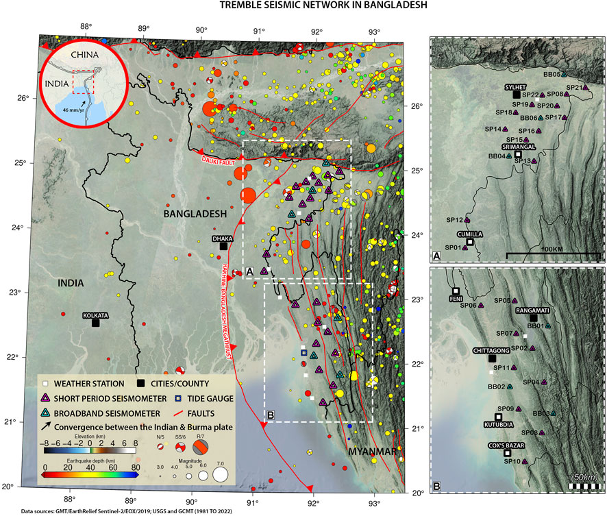
FIGURE 1. Map of Bangladesh showing stations in the TREMBLE network (triangles), weather stations (white squares), tide gauge (open square), major cities (black squares), major faults (red lines), earthquakes from the USGS catalogue (circles) (USGS, 2019) and focal mechanisms (beach-balls) (Dziewonski et al., 1981, Ekström et al., 2012). (A,B) show enlarged maps with labels for stations and cities. Inset: regional map showing plate boundary of Indian plate; arrow shows movement of Indian plate relative to Eurasian plate. Locations where weather stations and cities coincide are plotted as white boxes with a black outline.
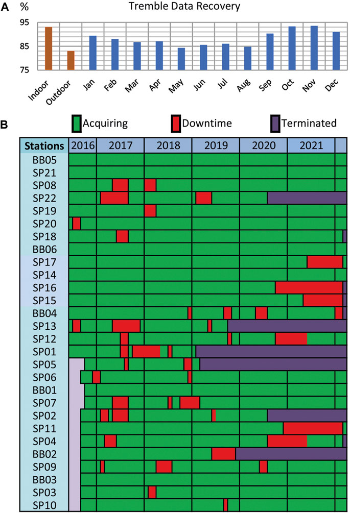
FIGURE 2. TREMBLE data recovery, (A) as a function of indoor/outdoor deployment styles and by month. (B) Acquisition success at each station. Stations are ordered by latitude (north to south, from top to bottom). Northern stations (BB05 to SP01); southern stations (SP05 to SP10). See locations of stations in Figure 1.
We classify stations into four categories based on their levels of representative anthropogenic noise (4–14 Hz). This is estimated by averaging daily anthropogenic noise levels recorded during November 2016 (in the dry season) and comparing the noise at individual sites with respect to the total noise across the whole network. Station information and anthropogenic noise information are listed in Supplementary Table S1.
2.2 Environmental data
To understand the sources of seismic noise across our network, we compare seismic noise recorded by TREMBLE with environmental data. We utilise weather stations operated by the Bangladesh Meteorological Department that record temperature, wind, and rainfall every 3 hours. Bangladesh experiences extreme variations in temperature, wind, and rainfall throughout the year due to the monsoon. It broadly experiences two seasons: the dry season (from October to April) and the wet season (from May to September) (Supplementary Figure S3). Warm seas lead to tropical storms and cyclones in the Bay of Bengal and land depressions near the coast; these storms generally occur from April to December, with a lull in July (Supplementary Figure S4).
We extract significant wave height and ocean wind speed in the Bay of Bengal from the global scale ocean wave model Wavewatch III (Tolman, 2009; Rascle and Ardhuin, 2013). We use ocean wind speeds downloaded from hindcasts produced by the United States National Weather Centre (https://polar.ncep.noaa.gov/waves/hindcasts). For significant wave height, we use the wave model, which includes wave reflections from coastlines. Significant wave height is a common statistical measure of wave height used in oceanography, defined as the mean wave height (trough to crest) of the highest third of the waves. We calculate mean significant wave height in the Bay of Bengal by extracting and averaging over that spatial region. We also use sea level data recorded by a tide gauge at Chittagong port obtained from the University of Hawaii Sea Level Center (Caldwell et al., 2015).
3 Methods
We characterise the site response for each station by using ambient noise to calculate the ratio of horizontal to vertical spectra (Nakamura, 1989; Nakamura, 2019). A peak in the horizontal to vertical spectral ratio (HVSR) corresponds to the resonance frequency and is related to the depth of strong impedance contrasts (such as the sediment–bedrock interface). HVSR peaks, often used as input for ground motion models (e.g., Zhao et al., 2006), result from a combination of S-wave resonance within the sedimentary section (Nakamura, 1989) and surface wave horizontal polarisation (Bonnefoy-Claudet et al., 2008).
HVSR is computed for each station using 2 weeks of data (in the dry season). Amplitude spectra are computed for each component in 50 s time segments using Welch’s averaged, modified periodogram method filtered with a Hamming window (Welch, 1967). We use a 50 s window to capture signals down to ∼0.2 Hz (10 cycles), to capture our lowest expected resonance frequency. For each time window, horizontal components are averaged using a geometric mean, and divided by the vertical component spectra. The average HVSR is calculated as the mean for all segments. Using over 24,000 segments, transient noise, such as earthquakes, have minimal influence. Results are validated using Geopsy software (Wathelet et al., 2020).
Background noise is analysed using probabilistic power spectral densities (PPSDs). The power spectral density (PSD) for each station and component is first computed from the discrete Fourier transform. PSDs represent the proportion of the total signal power contributed by each frequency component of a signal and are computed in units of decibels (dB) with respect to acceleration per frequency (m/s2)2/Hz. PSDs are then analysed statistically to produce probability density functions, following the method of McNamara and Buland (2004) implemented in Obspy (Beyreuther et al., 2010). We remove the instrument response and calculate PPSD’s in 30-min windows with 50% overlap. PPSDs are smoothed in period bins of half an octave. To investigate seasonal changes in noise, we extract the mean from PPSDs computed per day. To analyse specific frequencies, the required centre frequency is extracted from each daily mean PPSD function. Note that the amplitude at the centre frequency is an average over the period bin (Supplementary Table S2.) Variations in the horizontal to vertical ratio at specific frequencies are calculated from the mean daily power at each component. Horizontal components are averaged using a geometric mean. For long-term HVSR curves at specific frequencies, we remove outliers from the time series, defined as more than three MAD (median absolute deviations) away from the local median within a sliding window (usually 10 days).
We compute spectrograms to look at noise variations over short time windows. Spectrograms display power at different frequencies over time and are useful to identify signals from different sources [e.g., Lythgoe et al. (2021)]. Spectrograms are computed by calculating the short-term Fourier transform for overlapping time windows. We choose a time window of 600 s, balancing the need to account for the longest period signals of interest (∼100 s), while maintaining adequate time resolution.
4 Results
4.1 Site resonance frequencies
Following the HVSR interpretation guidelines in Acerra et al. (2004), we obtained clear HVSR peaks for only 11 stations; the rest had either no peak or a broad peak (Figure 3 shows illustrative example for several stations). Flat profiles or broad peaks indicate low impedance contrast beneath the station, for example, the presence of a thick sedimentary column where velocity gradually increases (Acerra et al., 2004). Since Bangladesh is covered in thick sediment, up to 15 or 20 km thick (Johnson and Nur Alam, 1991; Singh et al., 2016), low impedance contrast is unsurprising. Station SP04 displays a double peak, indicating heterogeneous subsurface structure; in this case we take the lowest frequency to represent the site resonance frequency, although the higher frequency peak is likely a secondary natural resonance frequency due to a shallower impedance contrast (Acerra et al., 2004). Stations with a single clear peak can be broadly placed into two groups: those with a resonance frequency of less than 1.5 Hz, generally located in the northern Sylhet region, and those with a resonance frequency greater than 2.5 Hz, generally located in the southern Chittagong region (Figure 4).
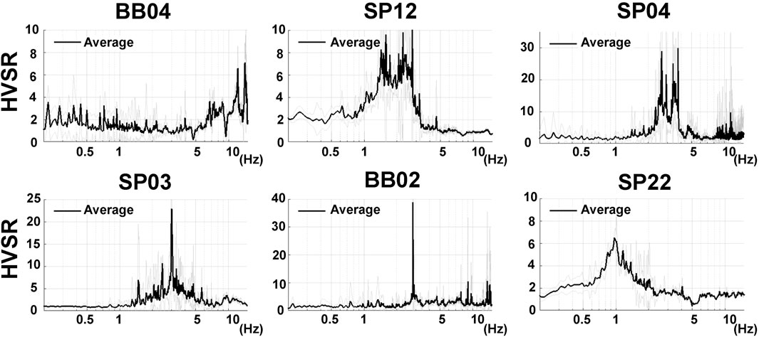
FIGURE 3. Horizontal Vertical Spectral Ratios (HVSR) for several stations. Shown are stations: BB04 (no peak), SP12 (broad peak), SP04 (multiple peaks), and SP03, BB02, SP22 (single peaks). The grey lines represent the upper and lower limits of standard deviation.
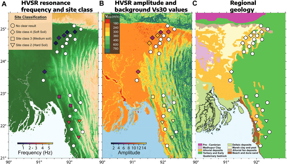
FIGURE 4. HVSR results for TREMBLE stations. Station colours correspond to resonance frequency (A) and amplitude (B), while station shapes correspond to the calculated site classification. (C) Shows the large-scale regional geology. The background map in (B) shows Vs30 data (McPhillips et al., 2020) derived from topography from U.S. Geological Survey (https://doi.org/10.5066/P9H5QEAC). The geological map in (C) is modified after Chowdhury et al., 2021; Limaye 2011.
Of the stations with a clear HVSR peak, they all exhibit a peak amplitude greater than five, with the southern stations having particularly high amplitudes. According to Nakamura (1996), Nakamura, (2019), high peak amplitudes correspond to high ground amplification (for hard ground the HVSR is ∼1, whereas for soft ground the HVSR is greater than 1). Nakamura (1996) further introduced the fragility index, calculated as the ratio of the squared amplification to the resonance frequency, which is large for high amplifications at low resonance frequencies. The fragility index has been shown to positively correlate to damage and liquefaction potential in several settings, including Japan, California, and India (Nakamura, 1997; Nakamura et al., 2014; Singh et al., 2017; Nakamura et al., 2014 analysed the correlation between fragility index and liquefaction in Tokyo following the 2011 Mw9.1 Tohoku earthquake and suggested that a fragility index above 12 corresponds to areas with high liquefaction risk. Other studies suggest fragility index values above 10 (Huang and Tseng, 2002) or 20 (Singh et al., 2017; Kang et al., 2021) are indicative of sites with high liquefaction potential. All our sites with a measurable HVSR peak have a fragility index exceeding 10, with several sites exceeding 100, which may represent a high risk of severe shaking and liquefaction in an earthquake. Helaly and Ansary (2021) also found high fragility index values (over 100) within Dhaka city. However, we caution that the amplitude of the HVSR peak also corresponds to the relative proportion of Love waves in the ambient noise field, not simply to horizontal ground amplification (Bonnefoy-Claudet et al., 2008). As we show later, the HVSR amplitude can vary depending on the season.
We classify our sites using the HVSR site classification scheme introduced by Zhao et al. (2006). Sites in southern Bangladesh generally fall within site class II, indicating hard soil, while sites in the north are exclusively site class IV, indicating soft soil (Figure 4). This is consistent with the northern sites typically being located on the Sylhet sedimentary basin, while the southern sites are located above the Bangladesh-Myanmar fold belt, which has uplifted and exhumed deeper rocks (Figures 4B, C).
4.2 Microseism signal identification
We first analyse and compare spectra during two periods: 1) in the dry season at the start of the year, and 2) in the monsoon season at the middle of year. We choose these two periods since they illustrate the largest annual changes in the noise spectrum in our study area. The comparison also helps to refine the frequencies of the microseisms and other signals of interest. We subsequently use these frequency ranges to investigate the long-term spatiotemporal variation of the signals.
4.2.1 Background noise levels in monsoon and dry seasons
Figure 5 shows PPSDs for a two-week period in the dry season (1st to 14th January 2018) and in the monsoon season (1st to 14th June 2018) for five example stations. We compare the PPSD’s with a reference noise model computed from analysis of global seismic stations, principally located within continental interiors (Peterson, 1993). The background noise at all stations is below the high-noise level (Figure 5), for both horizontal and vertical components (Supplementary Figure S5). Several stations located near urban areas approach the high-noise level at the frequency range of anthropogenic noise (∼3–15 Hz), for example, station SP20 (Figure 5), which is located close to a residential area. We do not find any correlation between noise levels and stations installed indoors or outdoors (Supplementary Figure S6).
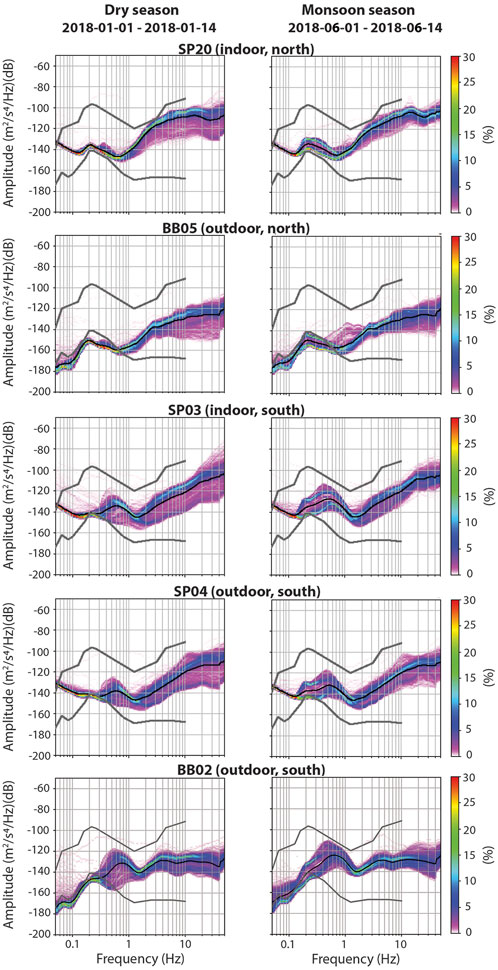
FIGURE 5. Probabilistic Power Spectral Densities (PPSDs) for the vertical component of several example stations for a two-week period in the dry season (left column), and monsoon season (right column). Grey solid lines mark the high and low noise limits from a reference noise model (Peterson, 1993). Horizontal components are shown in Supplementary Figure S5.
Stations in the south, near the coast, have a distinct bump of elevated energy between approximately 0.3–1 Hz, compared to stations further inland (Figure 5). This signal is persistent throughout the year, appearing in both dry and monsoon seasons, and likely represents the local microseism, which is generated near the coast. In the monsoon period, all stations in Figure 5 show elevated amplitudes at frequencies below 1 Hz. Figure 6 shows the difference in the mean PPSD between the monsoon and dry season for all stations. Between approximately 0.15 and 1 Hz, there is an increase in amplitude by ∼10 dB in the monsoon period. Broadband stations record an additional signal in the monsoon period at frequencies less than 0.15 Hz, approximately centred on 0.08 Hz, which matches the frequency range of the primary microseism. At higher frequencies (>1 Hz), stations SP02 and BB01 show increased amplitude in the monsoon period. This may be related to increased river discharge since these stations are located close to a major river. All energy differences between dry and monsoon periods are larger for southern compared to northern stations. We next compare spectrograms for these representative time periods, then discuss each of these signals in the following sections.
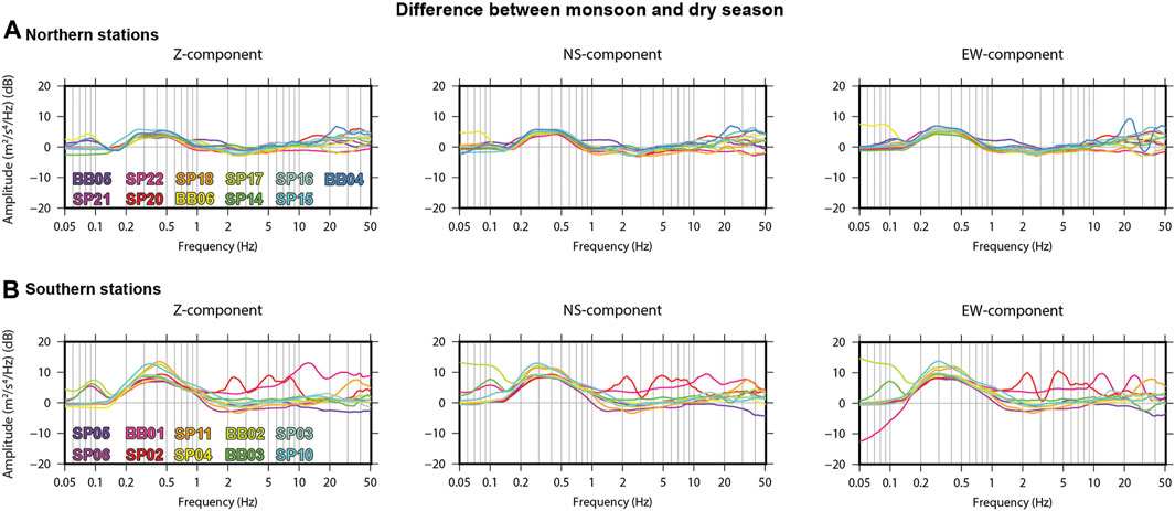
FIGURE 6. Difference in amplitude between power spectra in the monsoon and dry season. Positive values have larger amplitude in the monsoon season. All three components are shown with stations grouped into northern, inland (A) and southern, near the coast (B).
4.2.2 Spectrograms in the monsoon and dry seasons
In June 2018, a tropical depression developed in the Bay of Bengal near the Bangladesh coastline (India Meteorological Department, 2019). The depression moved onshore on June 10th, bringing heavy rainfall and strong winds to many areas of Bangladesh. Flooding was reported in the south-east of the country, triggering widespread evacuations and fatalities (European Commission’s Directorate-General for European Civil Protection and Humanitarian Aid Operations Report, 2018).
Figure 7 shows the spectrogram during this period recorded at station BB02, which is the closest broadband station to the coast (13 km). There is an increase in power at frequencies less than 1 Hz when the depression forms offshore and moves towards land. Between 0.4–0.8 Hz, the increase in power appears to be correlated with an increase in wind speed recorded at the nearest weather station. An increase in power at frequencies less than 0.05 Hz, particularly strong on the horizontal components, also appears to be correlated with wind. The secondary microseism is evident between ∼0.15–0.35 Hz. The microseism shows a gradual increase in power, which is similar to the increase in significant wave height and ocean wind speed. The peak frequency of the secondary microseism appears to decrease as the tropical depression develops. The primary microseism at ∼0.07–0.08 Hz is evident, though weak, and does not appear to increase in power during the tropical depression.
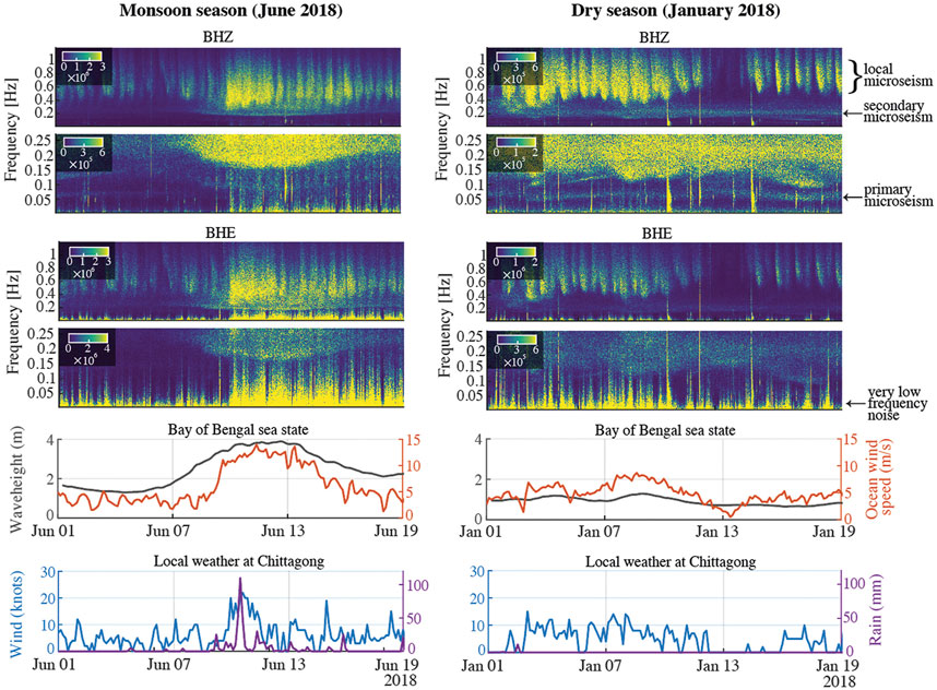
FIGURE 7. Spectrograms and environmental data in the monsoon season (June 2018, left column) and dry season (January 2018, right column). Seismic data is from BB02. For each component (BHZ and BHE shown) the top panel shows frequencies less than 1.2 Hz, and the bottom shows frequencies less than 0.27 Hz. Bay of Bengal Sea state is a spatial mean of data extracted from WAVEWATCH III hindcasts. Weather data are from Chittagong weather station.
Compared to during the depression, the spectrogram of a twenty-day period in the dry season shows less microseism energy (note the different colour scales in Figure 7). There is a striking drop in power between ∼0.4–0.8 Hz during a period of no wind. This energy at 0.4–0.8 Hz also appears to have cyclic behaviour. The secondary microseism (∼0.15–0.35 Hz) is evident, with constant power through the time period. The primary microseism (∼0.07–0.08 Hz) is also relatively constant in power and is more evident on the vertical component, although this is likely because the horizontal component is dominated by very low frequency energy (∼<0.05 Hz).
4.3 Spatiotemporal variations of different frequency signals
4.3.1 Local microseism (0.4–0.8 Hz) modulated by ocean tides
Spectrograms show that the amplitude of energy between ∼0.4–0.8 Hz, 1) increases when the tropical depression comes onshore and 2) markedly drops when there is no wind. We investigate long-term changes in this frequency range by extracting the mean power at 0.625 Hz (1.6 s period) from daily PPSDs. Figure 8 shows the daily changes at this frequency for the southern station BB03 (60 km from the coast) and the northern station BB05 (275 km from the coast). BB03 shows clear annual changes in power, with maxima in July (in the monsoon season), and minima in January (in the dry season). Annual changes at BB03 are on the order of 10 dB, while BB05 shows only very weak annual changes (on the order of several decibels, Supplementary Figure S7). The decay of the signal inland (also shown across the network in Figure 6) indicates that the signal is likely generated near the coast.
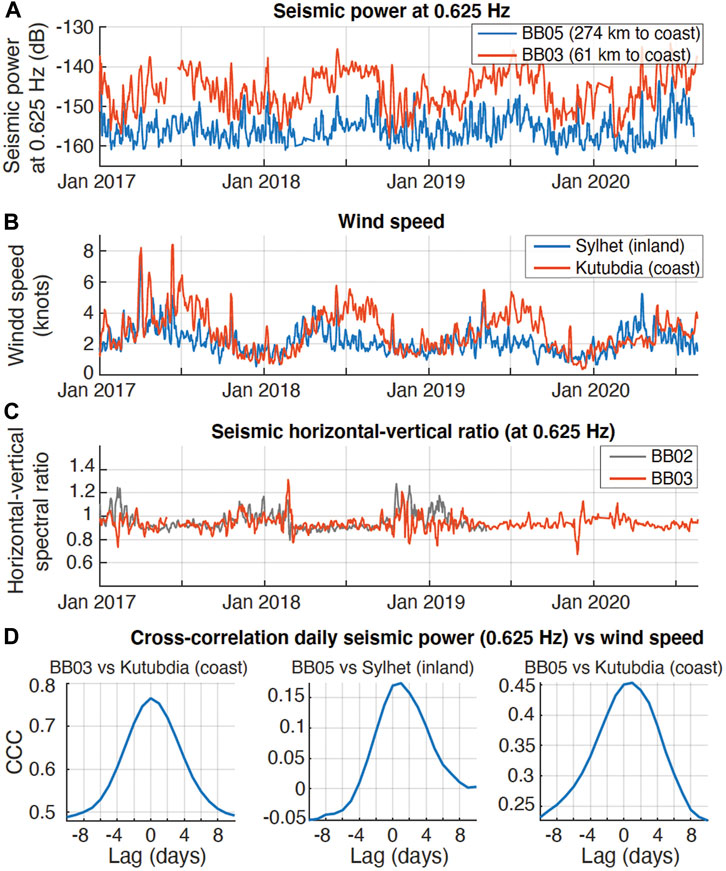
FIGURE 8. (A) Mean daily seismic power spectral density at 0.625 Hz for stations BB05 and BB03 on vertical component (units same as Figure 5). (B) Wind speed recorded at closest weather stations to BB05 (Sylhet) and BB03 (Kutubdia, on the coast). (C) Seismic horizontal to vertical spectral ratio at 0.625 Hz. (D) Cross-correlation functions between seismic power and wind speed. CCC=cross-correlation coefficient.
In the absence of a buoy located near shore, we use wind recorded at a coastal weather station to compare to seismic data. Figure 8 shows a positive correlation between coastal wind and seismic power at 0.625 Hz that is stronger than the correlation between seismic power and mean wave height throughout the Bay of Bengal (Supplementary Figure S8). The correlation is relatively strong for station BB03, with a maximum cross-correlation coefficient of 0.78 at a lag of 0 days. We compare seismic power at station BB05 with both local wind (recorded near the station) and coastal wind (∼325 km from the station). We find no correlation with local wind (cross-correlation coefficient of 0.17), while there is a weak correlation with coastal wind (maximum cross-correlation coefficient of 0.45 at 0 days lag), indicating the signal is likely generated near the coast. The period range and relationship with coastal wind conditions indicate that this energy is the local microseism (Becker et al., 2020, also called the short-period secondary microseism), which is generated by wind-driven ocean waves in near-coastal areas. We find that the horizontal to vertical ratio is approximately one (Figure 8C).
Figure 9 shows the raw seismic data, filtered to 0.4–0.8 Hz, and its envelope, at near-coast station BB02 in Chittagong. The seismic data are overlain with wind speed recorded at a coastal weather station, and the mean wind speed extracted from the ocean model in an area near the coast (Figure 9A). Higher wind speeds broadly correlate to higher seismic amplitude, as already discussed, although no strong short-term relationship is evident in Figure 9.
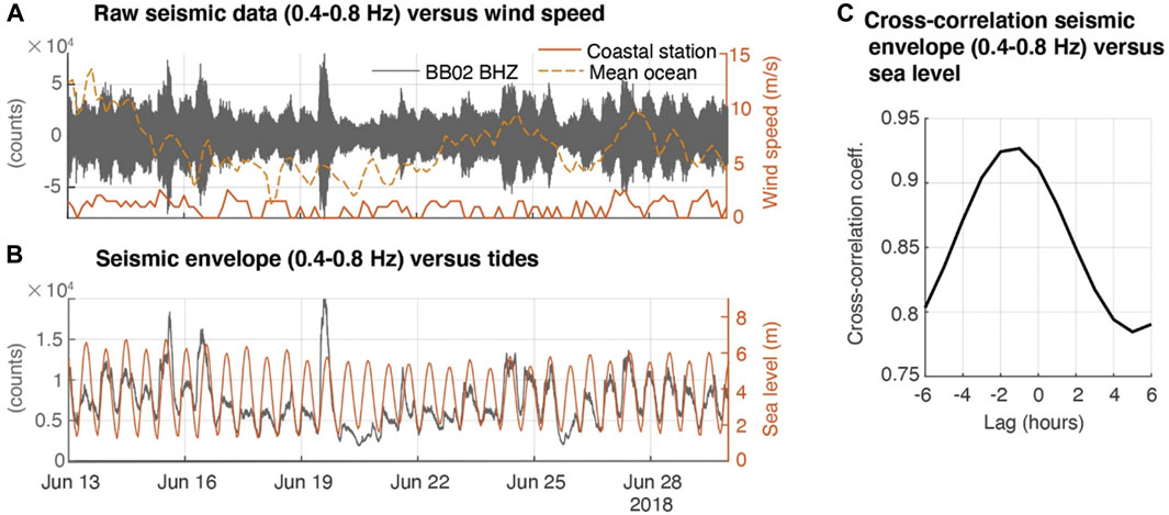
FIGURE 9. (A) Raw seismic data filtered 0.4–0.8 Hz on BHZ component of BB02 (black, left). Wind speed (right) recorded at coastal weather station Kutubdia (solid line) and the mean extracted from the ocean model (dashed line). (B) Seismic envelope of 0.4–0.8 Hz calculated in 15-min windows (black) versus sea level recorded at a local tide gauge (orange). Sea level in the bottom panel is shifted back by 1 hour. (C) Cross-correlation between seismic envelope and sea level shown in (B).
Cyclicity in the local microseism at a period of less than 1 day is shown in the spectrograms in Figure 7 and raw seismic data in Figure 9 The sea level recorded at a tide gauge at the nearby Chittagong port is overlain on seismic data in Figure 9B. The tide gauge data show a local tide with 12-hour cyclicity. There is a strong correlation between the sea level and seismic energy, with a cross-correlation of 0.93 at a lag of 1 h (Figure 9C), indicating that the microseism energy peak precedes the high tide by ∼ 1 h.
4.3.2 Secondary microseism (0.15–0.35 Hz) correlated with sea state in the Bay of Bengal
PPSD comparisons (Figure 6) and spectrograms (Figure 7) indicate that the secondary microseism occurs at frequencies between 0.15–0.35 Hz. The microseism amplitude appears to be correlated with the sea state in the Bay of Bengal (Figure 7), with higher amplitude and a slight shift to longer periods when the wave height is highest. We investigate longer-term changes in the power of the secondary microseism by extracting the mean power at 0.25 Hz from daily PPSDs (Figure 10; Supplementary Figure S9). This is compared to mean daily variations in significant wave height in the Bay of Bengal. We temporally smooth both time series with a 5-day moving window, which reduces the impact of anomalous one-day spikes in the seismic noise.
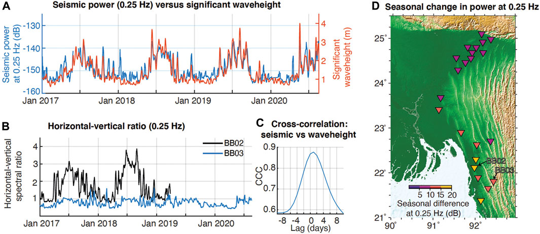
FIGURE 10. (A) Mean daily seismic power spectral density at 0.25 Hz on the vertical component of station BB03 (blue, units same as Figure 5, in dB), plotted with mean significant wave height in the Bay of Bengal (orange). (B) Horizontal-to-vertical ratio at 0.25 Hz at BB03 and BB02. (C) Cross-correlation between seismic (0.25 Hz) and significant wave height shown in (A). (D) Magnitude of seasonal change in seismic power at 0.25 Hz across the network between the monsoon and dry seasons.
Figure 10 shows a positive correlation between seismic power at 0.25 Hz and Bay of Bengal significant wave height, with a correlation coefficient of 0.87 at station BB03. Indeed, there is good correlation between variations in seismic power at 0.25 Hz between all stations in our network, shown for a sample six-month period at four stations in Supplementary Figure S10. All stations also record a seasonal change in the energy of the secondary microseism (Figures 6, 10). The secondary microseism is up to 20 dB ‘louder’ in the monsoon period near to the coast, decreasing to approximately 10 dB ‘louder’ inland. The seasonal variation is recorded at our most distant stations, up ∼275 km inland (Supplementary Figure S9). There is a lag of 1 day between the secondary microseism and significant wave height (Figure 10C), although the delay could be less than 1 day, as this is the temporal resolution in this analysis. The horizontal to vertical ratio at 0.25 Hz is approximately less than or equal to one at station BB03, while it is between one and four at station BB02 (Figure 10B). Seasonal changes are additionally evident for BB02, with greater horizontal energy in the monsoon period.
4.3.3 Primary microseism at ∼0.07–0.08 Hz
A comparison between PPSDs in the monsoon and dry seasons indicates an increase in noise at frequencies less than ∼0.1 Hz on broadband stations in the monsoon period (Figure 6), which corresponds with the primary microseism frequency range. The change in seismic power is highest for stations near the coast but is still recorded at our inland stations (Figure 6). Spectrograms in Figure 5 show that the primary microseism has a dominant frequency of 0.07–0.08 Hz. However, unlike the secondary microseism, there appears to be no increase in primary microseism power during a tropical depression, when the ocean wave height increases (Figure 7). We investigate long-term changes in primary microseism power by collating mean daily PSDs in Figure 11. Although there are changes in primary microseism power (up to 20 dB at station BB03, up to ∼10 dB at BB05, which is 273 km inland), there is no systematic seasonal variation or correlation with sea state. The primary microseism is believed to be generated at shallow water depths from shoaling of ocean waves on a sloping seafloor (Hasselmann, 1963), thus we also compare seismic power during tropical storms that occur in near-coastal areas of Bangladesh (Figure 11). There is little correspondence between times of tropical storms and changes in primary microseism power (Figure 11).
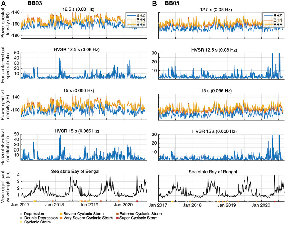
FIGURE 11. From top to bottom panels: daily mean power spectral density at 0.08 Hz; horizontal to vertical spectral ratio at 0.08 Hz; daily mean power spectral density at 0.066 Hz; horizontal to vertical spectral ratio at 0.066 Hz; mean significant wave height in the Bay of Bengal and times of tropical storms. (A) Station BB03 (60 km from the coast), (B) station BB05 (275 km from the coast).
Horizontal to vertical spectral ratios in the primary frequency range are much larger than one (Figure 11), indicating dominant horizontal energy. Interestingly, there is a seasonal change in the horizontal to vertical ratio, with greater horizontal energy near to times of low mean wave height (Supplementary Figure S10).
4.3.4 Very low frequency (<0.05 Hz) horizontal noise
Spectrograms in Figure 7 show high amplitude noise at frequencies less than 0.05 Hz, which is stronger on the horizontal than vertical components and present throughout the year. The amplitude increased when the tropical depression made landfall near the station, suggesting that the noise source is related to localised changes in atmospheric pressure (driving wind), rather than to ocean waves, which were elevated before the storm reached land.
Elevated noise on the horizontal components at 0.02–0.04 Hz occurs on all broadband stations (Figure 12; Supplementary Figure S11), including those located over 200 km inland. Figure 12 shows raw seismic data filtered to 0.02–0.04 Hz at stations BB02, BB03, and BB04 recorded over 20 days in January 2018. The vertical components are much quieter (by a factor of 10), showing only discrete spikes in noise related to regional or teleseismic earthquakes. Interestingly, a cyclic pattern is apparent in the horizontal noise. The envelope of the horizontal components highlights that the amplitude varies with a strong 24-h period. Stations BB02 and BB03 have elevated noise levels during the daytime (from approximately 10a.m. to 5p.m. local time), whereas BB04 has elevated noise during the night and morning (∼10p.m.–11a.m. local time). The different patterns between stations and lack of signal attenuation inland indicate the signal is not a microseism effect but is rather related to local conditions. Figure 12 compares the seismic power with changes in temperature and wind recorded at the nearest weather station to each seismic station. Temperature and wind also show daily periodicity, implying that these could be the origin of the noise. We investigate any long-term variations in the low-frequency signal in Supplementary Figure S13, which shows the mean daily PPSD at 0.03 Hz for 3.5 years of data for all broadband stations. No seasonal variations in the amplitude of the signal are evident, implying that it always persists.
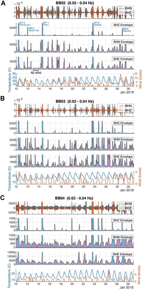
FIGURE 12. Temporal variations between 0.02–0.04 Hz for a 20-day period in January 2018, plotted in local time (UTC +6 h). (A) Station BB02, (B) BB03. (C) BB04. Top (first) panel of (A–C): raw seismic data filtered to 0.02–0.04 Hz. Middle (second to fourth) panels of (A–C): Envelope of 0.02–0.04 Hz filtered data, computed in one-hourly moving windows. Areas under curve are coloured blue at times of earthquakes, as highlighted on vertical components. Bottom (fifth) panel: Temperature and wind recorded at the closest weather station to each seismic station.
4.3.5 Impact of major river flow at 5 Hz
Station SP02 differs from the other stations in that it displays elevated power in the monsoon season at higher frequencies (Figure 6). There are two peaks, centred at approximately 2 Hz and 5 Hz (Figure 6). Station SP02 is located within 40 m of the major Karnaphuli river, which is the largest river in our study region and one of the fastest flowing rivers in Bangladesh (Figure 13A). The Karnaphuli river is located in the Chittagong region, with Bangladesh’s largest seaport at its mouth. Figure 13B shows the longer-term variation in seismic power at 2 and 5 Hz. Seasonal variations are evident at both frequencies, with greater seismic power in the monsoon season, however 5 Hz power shows the most consistent and pronounced seasonal trend. In the absence of river discharge data, we compare the seismic power to rainfall at the nearest weather station. There is a clear relationship, with increased power at 5 Hz following times of high rainfall (Figure 13B). The highest rainfall in 2018 occurs on June 11th and is followed by the peak seismic power on June 19th. Similarly, in 2019, peak rainfall occurs on 11th July and the peak seismic power follows on 20th July. Our observations indicate a delay of approximately 8 days between peak rainfall and maximum discharge in the lower course of the Karnaphuli River.
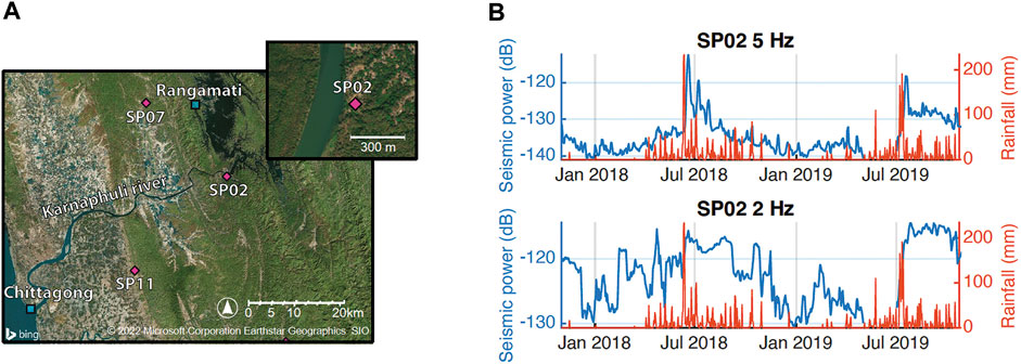
FIGURE 13. (A) Location of station SP02 (Supplementary Table S1). Seismic stations (pink), weather stations (blue). (B) Mean daily seismic power spectral density at 5 Hz (top) and 2 Hz (bottom) for the vertical component of SP02 (units same as Figure 5, in dB), plotted against rainfall recorded at Rangamati weather station.
Located ∼150 m from the Karnaphuli River, station BB01 also shows elevated power during the monsoon season at higher frequencies, as illustrated in Figure 6. However, despite the similarities in elevated power levels, these signals at BB01 do not exhibit any correlation with local rainfall (Supplementary Figure S14). Instead, these signals likely arise from instrumental issues, as indicated by the concurrent presence of anomalous low-frequency horizontal components during this time of elevated seismic power.
4.3.6 Anthropogenic variations in noise (∼3–14 Hz)
At frequencies above ∼3 Hz, seismic noise tends to be dominated by man-made sources near the seismic site, such as traffic, footfall, and machinery (McNamara and Boaz, 2019). Variations in seismic noise can therefore represent patterns in human movement. During our recording time to date, large changes in human movement in Bangladesh occurred during national holidays (such as Eid-al Fitr and Buddha Purnima) and the COVID-19 pandemic.
When the COVID-19 pandemic hit Bangladesh, the government declared several “General Holidays” to curb the spread of the virus. The first lockdown began on 26 March 2020 and included bans on transportation and closure of many workplaces; many migrant workers returned to their homes in the countryside. This lockdown ended on 30 May 2020, with more limited restrictions continuing until the 4 August 2020 (COVID-19 Timeline in Bangladesh, 2021). These restrictions were associated with sharp drops in community movement and led to associated changes in seismic noise (Supplementary Figure S15).
The TREMBLE network recorded varying changes in noise during the lockdown depending on anthropogenic activities and police enforcement (Figure 14). For example, station BB03, which is deployed outside a boarding school in a remote area, recorded a large drop in noise (4–14 Hz) during the lockdown, due to a reduction in outdoor activities and departure of many students. A (smaller) drop in noise is also seen during the end-of-year holiday. The highest change in noise during the COVID pandemic was at station SP04, which recorded a 54% reduction in noise immediately following the first lockdown. SP04 is in a common yard of a small tribal village, and the noise reduction reflects a drop in anthropogenic activities. Hourly noise data at this station (Supplementary Figure S16) suggest that before the lockdown, human activities usually ended around 5 p.m., but during the lockdown, activities extend to almost 7 p.m., perhaps to avoid crowded times.
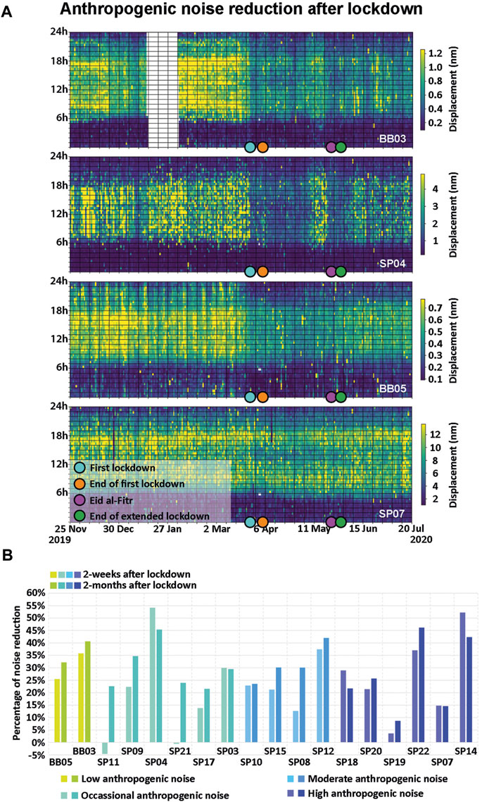
FIGURE 14. (A) Seismic amplitude in displacement between 4–14 Hz (Lecocq et al., 2020) for a time periods from November 2019 to July 2020 covering the COVID-19 pandemic lockdown measures in Bangladesh. Four representative stations are shown. (B) Percentage reduction of mean noise in a 2 week and two-month period after the lockdown measures, versus the mean noise in a two-week period before lockdown began.
The reduction of anthropogenic noise levels evolved over time during the lockdown. Figure 14B shows the reduction in noise between 2 weeks after lockdown and 2 months after lockdown. For stations at generally low anthropogenic noise sites, like BB05 and BB03, we see a reduction of about 25%–35% after 2 weeks and a further noise reduction of another 5% after 2 months. For stations in anthropogenically noisy areas, some show very large drops in noise, whereas at other stations the noise level remained roughly constant. For example, SP22 and SP14 exhibit a noise reduction of over 40%, likely because these stations are normally frequented by visitors (SP22 is at a resort, SP14 at a holiday home) whereas at SP19, noise levels dropped by less than 10%, since it is located in a residential area on the outskirts of Sylhet city. Generally, stations with occasional to moderate levels of anthropogenic noise exhibit a reduction of about 20%–30% regardless of whether they are in rural or urban areas (Supplementary Figure S19).
Distinctive changes in noise are normally associated with Eid-al-Fitr at most stations in our network. Stations that show noise reductions at Eid-al-Fitr include SP01, SP06, and BB04, located at a university, a rubber plantation, and a tea factory, respectively (Supplementary Figure S20). SP22, located in a resort in Sylhet city, shows a large noise reduction (Supplementary Figure S20), since the resort closes in this religious period. Unlike other stations, SP22 is normally noisiest at night, likely due to machinery such as a generator, which is switched off when there are no visitors (Supplementary Figure S20). SP19 does not show a significant noise change with Eid-al-Fitr itself, however there is a distinctive increase in noise between 2–4 a.m. during the prior fasting month of Ramadan reflecting the Night Vigil Prayer, completed before fasting begins at sunrise (Supplementary Figures S18, S20). The 2–4 a.m. signal is also seen at SP21 and occurs only during the month of Ramadan (Supplementary Figure S20). More in-depth analysis of the changes in anthropogenic noise throughout the network can be found in Supplementary Text S1.
5 Discussion and conclusion
Data recovery at TREMBLE stations was highly variable, even with regular station maintenance. We had the least success obtaining data from outdoor stations, with station performance principally depending on environmental factors. We have documented recommended best practices for station installation and maintenance in similar tropical areas based on our experience in Supplementary Table S3. All stations have ambient noise levels below the Peterson New Noise Model (Peterson, 1993), although there are considerable variations with frequency, location, and season. Table 1 provides an overview of the frequencies of the microseisms and other signals of interest in the region.
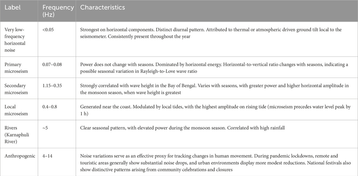
TABLE 1. Overview of signals studied and their characteristics.
Analysis of horizontal to vertical spectral ratios indicate that TREMBLE sites in the north are class IV (soft soil), whereas in the south they are generally class II (hard soil), which matches the known geology of Bangladesh. Site resonance frequencies vary between approximately 0.9 and 4 Hz, although many stations did not have a clear HVSR peak, indicating that they are located above a thick sedimentary column with little impedance contrast. We find high HVSR amplitudes (>5) at all stations with a measurable peak, with correspondingly high fragility indices. The identification of high fragility indices serves as a clear indicator of an elevated risk of liquefaction and severe shaking in an earthquake. Sites in the north on soft soil coincide with the highest seismic hazard in the region in terms of expected ground motion (BNBC, 2020). Future studies should be directed towards determining site classification and expected ground motion in the very densely populated areas of northern Bangladesh.
In the microseism frequency band, stations from the coast to far inland displayed two peaks, at around 0.08 and 0.25 Hz, corresponding to the primary and secondary microseism, respectively. These frequencies are higher than the global average of around 0.07 and 0.14 Hz, respectively (e.g., Stutzmann et al., 2000), likely due to shorter ocean wave wavelengths caused by the restricted fetch in the marginal sea of the Bay of Bengal.
A local microseism between 0.4–0.8 Hz is generated by wave interactions near the coast in the Bay of Bengal, with its amplitude strongest at stations near the coast. There is a positive correlation between local microseism power and coastal wind when comparing daily signals over a multi-year time scale (Figure 8). This is true for coastal and inland stations (Figure 8). However, no strong short-term relationship is evident when directly comparing raw seismic data and coastal wind speed data (Figure 9). This differs from Zhang et al. (2009), who found a strong correlation between local microseism amplitude and near-coast wind speeds, recorded by a buoy located near shore in California. The lack of strong short-term correlations in Bangladesh is likely because we do not have good observations of offshore oceanic windspeed: the weather station is located on land, and the ocean model does not have sufficient resolution.
The horizontal-vertical spectral ratio of the local microseism is approximately one, indicating a dominance of Rayleigh waves in the local microseism wavefield. Examining the local microseism in Australia (0.325–0.725 Hz), Gal et al. (2015) find that Rayleigh waves also dominate, although Love waves increasingly contribute at higher frequencies, possibly due to the conversion of Rayleigh waves at irregular coastlines, as also argued by Koper et al. (2010). Further analysis is needed to show if Love waves make up a small, possibly frequency dependent, component of the local microseism in Bangladesh.
Additionally, we observe a modulation of the locally generated seismic wave energy with ocean tides, with the microseism peak preceding high tide by ∼1 h. Our results are consistent with Becker et al. (2020), who find a local microseism (at 0.2–1 Hz) in the southern North Sea, with a peak in amplitude that precedes the water level maximum recorded at a nearby tide gauge. Wide shallow waters in both the Bay of Bengal and the North Sea are expected to produce larger amplitude and shorter wavelength tides than in the deep ocean, which may explain why there is a clear correlation between a local microseism and ocean tides in these locations. Becker et al. (2020) interpret the observed local microseism as generated in shallow water at near coastal areas, due to the interaction of incoming wave activity and tidal currents. This is consistent with our observation that high coastal wind speeds are needed to generate the local microseism and that the microseism power is highest on a rising tide, indicating that large wave heights in shallow, tidal areas are necessary to produce the local microseism. The observed time lags between microseism and water level peaks could be due to the microseism being generated in a different location to where the tide gauge is located and/or the dominant influence being when the tide is at the fastest velocity, rather than peak water level. Further work to precisely locate the microseism using array beamforming, as well as ideally using a tidal model rather than point measurement from a tide gauge, is needed to better understand its generation mechanism.
The power of the secondary microseism in Bangladesh is strongly correlated with mean significant wave height in the Bay of Bengal (Figure 10). The power changes with seasons, with up to 20 dB difference between monsoon and dry seasons recorded by coastal stations, and ∼5 dB seasonal difference recorded by stations >200 km inland. As wave height increases in a tropical depression, the secondary microseism power increases, and the frequency decreases. This is because it takes bigger storms (with greater wind speed, length, and duration of fetch) to generate ocean waves with longer periods (Bromirski et al., 1999), and may partially be due to the movement of the source areas of the secondary microseism to shallow water depths (Kedar et al., 2008). There is a lag of 1 day between the secondary microseism power and significant wave height (Figure 10C). A delay in seismic microseism amplitude with respect to significant wave height has been attributed to complex interactions between the incoming ocean swell with coastal reflections (Bromirski et al., 1999; Ardhuin et al., 2012).
There is a seasonal dependence of the horizontal-vertical ratio (between ∼1–4) at station BB02, whereas the horizontal-vertical ratio at station BB03 is nearly constant over time at 0.6–1. Generally, the secondary microseism is dominantly composed of Rayleigh waves (Stutzmann et al., 2009) due to its generation mechanism (Longuet-Higgins, 1950). However, in some cases the secondary microseism has strong horizontally polarised energy due to Love waves (e.g., Juretzek and Hadziioannou, (2016); Xiao et al., 2018), which are thought to be generated by steep bathymetry and subsurface geological boundaries (such as sedimentary basins), or through conversion from Rayleigh waves at heterogeneities along the microseism path (Gualtieri et al., 2020; Le Pape et al., 2021). BB02 shows increased horizontal energy in the monsoon period when wave height is highest, indicating a greater component of Love wave energy at this time. This may indicate that the location of the secondary microseism generating source changes by season, possibly due to tropical storms, which are frequent in the Bay of Bengal during the monsoon. Different Rayleigh-to-Love wave ratios between stations has been documented in several studies (Nishida et al., 2008; Juretzek and Hadziioannou, 2016), and a weak seasonal variation for a coastal region of California is reported by Tanimoto et al. (2016). BB02 is close to the coast, similar to the station analysed by Tanimoto et al. (2016), who suggested that the propagation distance at a near-coast station may be too short to create a diffuse wavefield at these long wavelengths.
The primary microseism shows positive horizontal to vertical spectral ratios, suggesting a significant non-Rayleigh wave contribution to the primary microseism in Bangladesh. The primary microseism has been found to contain dominant horizontal motion in other regions, due to horizontally polarised Love waves [e.g., Nishida et al. (2008); Juretzek and Hadziioannou, (2016)]. Unlike the secondary microseism, Love waves are generated directly in the primary microseism, likely from shear traction due to the shoaling of waves on inclined seafloor topography (Saito, 2010; Ardhuin, 2018). While the primary microseism power displays no strong seasonal changes, the horizontal to vertical ratio does, with higher horizontal energy in the dry season. The ratio of Love to Rayleigh waves in the primary microseism depends on the local source topography as well as the azimuth of the station with respect to the source, since Rayleigh waves and Love waves radiate differently (Ardhuin et al., 2015; Juretzek and Hadziioannou, 2016). Therefore, a changing horizontal to vertical spectral ratio could indicate a changing source location of the primary microseism with different seasons. Temporal trends in the horizontal-vertical ratio for the primary microseism are different to that of the secondary microseism–for example, BB03 displays no temporal variation for horizontal-vertical ratio in the secondary microseism, but a clear temporal variation for the primary. Further work is necessary to ascertain the source locations of the primary and secondary microseisms and how they change over time.
Large amplitude horizontal noise with a 24-hour periodicity is prevalent on all of our broadband stations at frequencies less than 0.05 Hz. A diurnal pattern in horizontal noise power at frequencies less than 0.05 Hz has previously been documented (Beauduin et al., 1996; Wilson et al., 2002; Koper and Hawley, 2010; De Angelis and Bodin, 2012; Wolin et al., 2015). Wilson et al. (2002) find no spatial correlation in long-period noise between regional stations, and conclude that the noise source must be local, from thermal or atmospheric driven ground tilt. Beauduin et al. (1996) and Wolin et al. (2015) utilise a co-located barometer to correlate the variation in long-period noise with atmospheric pressure. They conclude that this noise is likely produced by the elastic response of the Earth to atmospheric pressure fluctuations and wind, as proposed by Sorrells (1971). Atmospheric tides modulate surface pressure and wind speed. In particular, a large-scale atmospheric convective cell produces a 24-h periodic cycle (Dai and Deser, 1999). In continental areas, wind speed tends to peak in the afternoon, influenced by heating from the ground surface, and drops at night (Dai and Deser, 1999). This is similar to the pattern recorded in Bangladesh: for example, weather stations Kutubdia (near BB03) and Srimangal (near BB04) show that temperature and wind speed have a 24-hour cyclicity with peaks in the afternoon and low or no wind recorded at night (Figure 12). Chittagong weather station is on the coast and is likely influenced by coastal winds, so does not show a clear 24-hour cyclicity in wind speed. Peaks in horizontal seismic power for BB02 and BB03 occur during high winds (Figure 12), supporting the generation of this noise by instrument tilt due to the elastic response of the Earth to atmospheric pressure fluctuations. However, high seismic power for BB04 occurs during the night, which is not correlated with high wind at the nearest weather station (Figure 12C). BB04 also has extremely large power on the east-west component, ten times larger than the north-south component; this is likely an instrumental issue, since it first appears in June 2017 and then persists (Supplementary Figure S12). The station is located 14 km from the weather station, and on top of an exposed hill, so may experience local weather patterns–without a co-located barometer it is not clear why BB04 shows a different pattern than the other stations.
Wolin et al. (2015) note that the amplitude of the power change varies depending on the time of year and the soil conditions at the station: stations installed in fine silt material show the largest diurnal noise change, strongest in the summer months when the ground is dry (May-August in their location). Our stations in Bangladesh may therefore be particularly susceptible to atmospheric pressure variations, since they are often installed in shallow ground made of loose sediment. Stations installed indoors also record this diurnal noise change, although these indoor installations are not sealed from the outside and are often placed directly on the ground (e.g., Supplementary Figure S1). Installing seismometers at depth or in a vault can reduce long-period noise from atmospheric perturbations, but even in these deployments the noise cannot be completely removed [e.g., Wolin et al. (2015)], while budget and infrastructure constraints make boreholes unsuitable for many regional networks like TREMBLE. We do not see any seasonal variation in mean daily noise at < 0.05 Hz at the broadband sites in Bangladesh (Supplementary Figure S12).
Station SP02, which is located within 40 m of the major Karnaphuli River, records significant seasonal changes in seismic noise at ∼ 5 Hz. High seismic power occurs ∼8 days after high rainfall. The delay between local rainfall and seismic power is explained by the wide drainage area of the major Karnaphuli River, since river discharge is controlled by run-off from a wide area including the Indo-Burmese Mountains. Future stations located near large rivers in Bangladesh will also record high noise levels during the rainy season at frequencies up to ∼5 Hz, and this should be a consideration for future deployments.
Seismic noise due to anthropogenic activities is site specific. The seismic noise changes recorded by TREMBLE during the COVID pandemic demonstrate that lockdown measures were largely followed in most parts of Bangladesh, although a few stations were unaffected by lockdown measures. Roy et al. (2021) investigated pandemic lockdown noise changes at sites in remote areas of Gujarat, India, also finding negligible changes at some sites. Proximity to police stations appears to be one factor controlling the amount of noise reduction, with stations close to police stations showing large reductions (e.g., BB03), whereas those in tribal areas with little police influence show smaller noise reduction (e.g., SP07). We find that stations with the least reduction in seismic noise are located in highly populated urban locations (e.g., SP19), with more significant noise reduction in less populated areas (e.g., BB05); this may be due to the high population density in Bangladesh’s cities, where physical lockdowns may not be practically possible. Seismic noise is also affected by national holidays and religious events, particularly Eid-al-Fitr and Buddha Purnima. Many stations record a noise decrease during these holidays, including stations SP01, BB03, and BB04, located at a university, boarding school, and tea factory, respectively, while other stations report a noise increase, such as BB05, located at a rural resort. These patterns were largely reversed during the 2020 lockdown, reflecting that people could not leave their residence in the 2020 holiday period and festivals were instead celebrated locally.
Our study yields valuable insights into the multifaceted realm of seismic and environmental conditions in Bangladesh, with implications for research across diverse fields, including seismic deployments, seismic hazard, and imaging studies. Seasonal changes in background noise may manifest as seasonal changes in the amount and lower magnitude bound of detected seismicity. It has been observed, notably in Nepal and India, that earthquakes are more frequent in the dry season than the monsoon season, possibly due to loading from the summer monsoon’s rain supressing tremors (Bollinger et al., 2007). However, careful analysis of seismic noise and seismicity changes is required to fully account for changing noise on seismicity detection. Spatiotemporal noise variations also impact imaging studies. Seismic interferometry methods commonly assume a diffuse wavefield, which we have shown is not the case in the microseism frequency band in Bangladesh. Interferometry studies should particularly note the presence of high amplitude noise from the coast in the local microseism band which may bias resulting Green’s functions.
Further investigations of microseisms recorded in Bangladesh has the potential to improve our understanding of the generation of microseisms in a marginal sea setting like the Bay of Bengal. Additionally, the high number of tropical storms that occur in the Bay of Bengal and have been recorded by TREMBLE (∼35 from 2017–2021 including the strongest super cyclonic storms), present the opportunity to better understand storm generated microseism, and how microseism strength and frequency is affected by cyclone speed, water depth, coastal geometry, bathymetry, and crustal structures [e.g., Lin et al. (2017); Retailleau and Gualtieri, (2019); Park and Hong, (2020)]. Our analysis of one tropical storm raises several topics for further investigation, including why the frequency of the secondary microseism decreases as the tropical depression moves landwards, and why the primary microseism does not change in power or frequency as the depression strengthens. To improve our understanding of the microseisms identified here, future work to constrain the exact source locations is needed Further investigations into the composition of the wavefield would also give greater insight into the generation of microseisms. In particular, the changing horizontal-vertical ratio of the primary and secondary microseism might indicate a seasonal change in the dominant source generation location.
Data availability statement
The original contributions presented in the study are included in the article/Supplementary Material, further inquiries can be directed to the corresponding author.
Author contributions
SB: Conceptualization, Formal analysis, Investigation, Project administration, Writing–original draft, Writing–review and editing. KL: Conceptualization, Formal analysis, Funding acquisition, Investigation, Methodology, Project administration, Software, Supervision, Writing–original draft, Writing–review and editing. MM: Investigation, Writing–review and editing. SA: Writing–review and editing. JH: Funding acquisition, Writing–review and editing.
Funding
The author(s) declare financial support was received for the research, authorship, and/or publication of this article. This research was supported by the Earth Observatory of Singapore, the National Research Foundation of Singapore, and the Singapore Ministry of Education under the Research Centres of Excellence initiative. This research was funded in part by NERC award NE/W008289/1. For the purpose of open access, the author has applied a creative commons attribution (CC BY) licence to any author accepted manuscript version arising.
Acknowledgments
We use open-source software GMT (Wessel et al., 2019), python library ObsPy (https://github.com/obspy/obspy), Tectoplot (https://github.com/kyleedwardbradley/tectoplot-examples) and SeismoRMS (Lecocq, 2021). Bangladesh weather data was obtained from the Bangladesh Meteorological Department at http://www.bmddataportal.com/ (last accessed April 2023). Tide data is from: http://uhslc.soest.hawaii.edu/data/?rq#uh124a (accessed 16 August 2022). Ocean windspeed data are from Wavewatch III hindcast downloaded from https://polar.ncep.noaa.gov/waves/hindcasts/multi_1. Wave height calculated with a reflective coast is obtained from ftp://ftp.ifremer.fr/ifremer/ww3/HINDCAST. We thank Rahul Bhattacharya, U Mong Shing, Mir Md. Tasnim Alam, Alamgir Hosain Sohag, Atik Ullah Bulbul, Tariqul Islam, Md. Samiul Alim, Sangju Singha, Rafael Almeida, and Anna Foster for their contribution to TREMBLE. Additionally, we extend our appreciation to Mr. Yves Descatoire for his contribution to Supplementary Figure S1 and to Mari Hamahashi for her contributions to Figure 1 and Figure 4.
Conflict of interest
The authors declare that the research was conducted in the absence of any commercial or financial relationships that could be construed as a potential conflict of interest.
Publisher’s note
All claims expressed in this article are solely those of the authors and do not necessarily represent those of their affiliated organizations, or those of the publisher, the editors and the reviewers. Any product that may be evaluated in this article, or claim that may be made by its manufacturer, is not guaranteed or endorsed by the publisher.
Supplementary material
The Supplementary Material for this article can be found online at: https://www.frontiersin.org/articles/10.3389/feart.2024.1334248/full#supplementary-material
References
Acerra, C., Aguacil, G., Anastasiadis, A., Atakan, K., Azzara, R., Bard, P. Y., et al. (2004). Guidelines for the implementation of the H/V spectral ratio technique on ambient vibrations measurements, processing and interpretation. No. European Commission–EVG1-CT-2000-00026 SESAME. Brussels, Belgium: European Commission.
Akhter, S. H., (2010). Earthquakes of Dhaka. Environment of Capital Dhaka—plants wildlife gardens parks air water and earthquake, pp.401–426.
Antoniazza, G., Dietze, M., Mancini, D., Turowski, J. M., Rickenmann, D., Nicollier, T., et al. (2023). Anatomy of an alpine bedload transport event: a watershed-scale seismic-network perspective. J. Geophys. Res. Earth Surf. 128 (8), e2022JF007000. doi:10.1029/2022jf007000
Ardhuin, F. (2018). Large-scale forces under surface gravity waves at a wavy bottom: a mechanism for the generation of primary microseisms. Geophys. Res. Lett. 45 (16), 8173–8181. doi:10.1029/2018gl078855
Ardhuin, F., Balanche, A., Stutzmann, E., and Obrebski, M. (2012). From seismic noise to ocean wave parameters: general methods and validation. J. Geophys. Res. Oceans 117 (C5). doi:10.1029/2011jc007449
Ardhuin, F., Gualtieri, L., and Stutzmann, E. (2015). How ocean waves rock the Earth: two mechanisms explain microseisms with periods 3 to 300 s. Geophys. Res. Lett. 42 (3), 765–772. doi:10.1002/2014gl062782
Ayala-Garcia, D., Curtis, A., and Branicki, M. (2021). Seismic interferometry from correlated noise sources. Remote Sens. 13 (14), 2703. doi:10.3390/rs13142703
Beauduin, R., Lognonné, P., Montagner, J. P., Cacho, S., Karczewski, J. F., and Morand, M. (1996). The effects of the atmospheric pressure changes on seismic signals or how to improve the quality of a station. Bull. Seismol. Soc. Am. 86 (6), 1760–1769. doi:10.1785/bssa0860061760
Becker, D., Cristiano, L., Peikert, J., Kruse, T., Dethof, F., Hadziioannou, C., et al. (2020). Temporal modulation of the local microseism in the North Sea. J. Geophys. Res. Solid Earth 125 (10), e2020JB019770. doi:10.1029/2020jb019770
Beyreuther, M., Barsch, R., Krischer, L., Megies, T., Behr, Y., and Wassermann, J. (2010). ObsPy: a Python toolbox for seismology. Seismol. Res. Lett. 81 (3), 530–533. doi:10.1785/gssrl.81.3.530
BNBC (2020). Bangladesh National Building Code. Government of the People’s Republic of Bangladesh, Ministry of Housing and Public Works
Bollinger, L., Perrier, F., Avouac, J. P., Sapkota, S., Gautam, U. T. D. R., and Tiwari, D. R. (2007). Seasonal modulation of seismicity in the Himalaya of Nepal. Geophys. Res. Lett. 34 (8). doi:10.1029/2006gl029192
Bonnefoy-Claudet, S., Köhler, A., Cornou, C., Wathelet, M., and Bard, P. Y. (2008). Effects of Love waves on microtremor H/V ratio. Bull. Seismol. Soc. Am. 98 (1), 288–300. doi:10.1785/0120070063
Bromirski, P. D., Flick, R. E., and Graham, N. (1999). Ocean wave height determined from inland seismometer data: implications for investigating wave climate changes in the NE Pacific. J. Geophys. Res. Oceans 104 (C9), 20753–20766. doi:10.1029/1999jc900156
Bürgi, P., Hubbard, J., Akhter, S. H., and Peterson, D. E. (2021). Geometry of the décollement below eastern Bangladesh and implications for seismic hazard. J. Geophys. Res. Solid Earth 126 (8), e2020JB021519. doi:10.1029/2020jb021519
Burtin, A., Bollinger, L., Vergne, J., Cattin, R., and Nábělek, J. L. (2008). Spectral analysis of seismic noise induced by rivers: a new tool to monitor spatiotemporal changes in stream hydrodynamics. J. Geophys. Res. Solid Earth 113 (B5). doi:10.1029/2007jb005034
Caldwell, P. C., Merrifield, M. A., and Thompson, P. R. (2015). Sea level measured by tide gauges from global oceans–the joint archive for sea level holdings (NCEI accession 0019568), Version 5.5, NOAA national centers for environmental information, dataset. Centers Environ. Inf. Dataset. 10, V5V40S7W.
Chen, Y. N., Gung, Y., You, S. H., Hung, S. H., Chiao, L. Y., Huang, T. Y., et al. (2011). Characteristics of short period secondary microseisms (SPSM) in Taiwan: the influence of shallow ocean strait on SPSM. Geophys. Res. Lett. 38 (4). doi:10.1029/2010gl046290
Chowdhury, K., Hossain, Md, and Khan, Md. (2021). Introduction to Bangladesh geosciences and resources potential. doi:10.1201/9781003080817-1
COVID-19 Timeline in Bangladesh (2021). COVID-19 timeline in Bangladesh | betterwork.org. Available at: https://betterwork.org/portfolio/covid-timeline-in-bangladesh/ (Accessed October 13, 2021).
Dai, A., and Deser, C. (1999). Diurnal and semidiurnal variations in global surface wind and divergence fields. J. Geophys. Res. Atmos. 104 (D24), 31109–31125. doi:10.1029/1999JD900927
De Angelis, S., and Bodin, P. (2012). Watching the wind: seismic data contamination at long periods due to atmospheric pressure-field-induced tilting. Bull. Seismol. Soc. Am. 102 (3), 1255–1265. doi:10.1785/0120110186
Díaz, J. (2016). On the origin of the signals observed across the seismic spectrum. Earth-Science Rev. 161, 224–232. doi:10.1016/j.earscirev.2016.07.006
Dziewonski, A. M., Chou, T.-A., and Woodhouse, J. H. (1981). Determination of earthquake source parameters from waveform data for studies of global and regional seismicity. J. Geophys. Res. 86, 2825–2852. doi:10.1029/JB086iB04p02825
Ekström, G., Nettles, M., and Dziewonski, A. M. (2012). The global CMT project 2004–2010: centroid-moment tensors for 13,017 earthquakes. Phys. Earth Planet. Inter. 200–201, 1–9. doi:10.1016/j.pepi.2012.04.002
European Commission's Directorate-General for European Civil Protection and Humanitarian Aid Operations Report (2018). Bangladesh – floods and landslides (DG ECHO, BMD, disaster management and relief Ministry Bangladesh, local media). Available at: https://reliefweb.int/report/bangladesh/bangladesh-floods-and-landslides-dg-echo-bmd-disaster-management-and-relief (Accessed August 17, 2022).
Gal, M., Reading, A. M., Ellingsen, S. P., Gualtieri, L., Koper, K. D., Burlacu, R., et al. (2015). The frequency dependence and locations of short-period microseisms generated in the Southern Ocean and West Pacific. J. Geophys. Res. Solid Earth 120 (8), 5764–5781. doi:10.1002/2015jb012210
Gualtieri, L., Bachmann, E., Simons, F. J., and Tromp, J. (2020). The origin of secondary microseism Love waves. Proc. Natl. Acad. Sci. 117 (47), 29504–29511. doi:10.1073/pnas.2013806117
Gutenberg, B. (1936). On microseisms. Bull. Seismol. Soc. Am. 26 (2), 111–117. doi:10.1785/bssa0260020111
Hasselmann, K. (1963). A statistical analysis of the generation of microseisms. Rev. Geophys. 1 (2), 177–210. doi:10.1029/rg001i002p00177
Helaly, A. L., and Ansary, M. A. (2021). Assessment of seismic vulnerability index of RAJUK area in Bangladesh using microtremor observations. Soils Rocks 44, 1–13. doi:10.28927/sr.2021.057420
Hossain, B., Sohel, M. S., and Ryakitimbo, C. M. (2020). Climate change induced extreme flood disaster in Bangladesh: implications on people's livelihoods in the Char Village and their coping mechanisms. Prog. Disaster Sci. 6, 100079. doi:10.1016/j.pdisas.2020.100079
Huang, H.-C., and Tseng, Y.-S. (2002). Characteristics of Soil liquefaction using H/V of Microtremors in Yuan-Lin area,Taiwan. TAO 13 (3), 325–338.
India Meteorological Department (2019). Annual report on cyclonic disturbances over north Indian ocean in 2018. Available at: https://rsmcnewdelhi.imd.gov.in/uploads/report/27/27_60dae9_rsmc-2018.pdf (Accessed August 17, 2022).
Johnson, S. Y., and Nur Alam, A. M. (1991). Sedimentation and tectonics of the Sylhet trough, Bangladesh. Geol. Soc. Am. Bull. 103 (11), 1513–1527. doi:10.1130/0016-7606(1991)103<1513:satots>2.3.co;2
Juretzek, C., and Hadziioannou, C. (2016). Where do ocean microseisms come from? A study of Love-to-Rayleigh wave ratios. J. Geophys. Res. Solid Earth 121 (9), 6741–6756. doi:10.1002/2016jb013017
Kang, S. Y., Kim, K. H., Choi, M., and Park, S. C. (2021). Ground vulnerability derived from the horizontal-to-vertical spectral ratio: comparison with the damage distribution caused by the 2017 ML 5.4 Pohang earthquake, Korea. Near Surf. Geophys. 19 (2), 155–167. doi:10.1002/nsg.12150
Kedar, S., Longuet-Higgins, M., Webb, F., Graham, N., Clayton, R., and Jones, C. (2008). The origin of deep ocean microseisms in the North Atlantic Ocean. Proc. R. Soc. A Math. Phys. Eng. Sci. 464, 777–793. doi:10.1098/rspa.2007.0277
Koper, K. D., and de Foy, B. (2008). Seasonal anisotropy in short-period seismic noise recorded in South Asia. Bull. Seismol. Soc. Am. 98 (6), 3033–3045. doi:10.1785/0120080082
Koper, K. D., and Hawley, V. L. (2010). Frequency dependent polarization analysis of ambient seismic noise recorded at a broadband seismometer in the central United States. Earthq. Sci. 23, 439–447. doi:10.1007/s11589-010-0743-5
Koper, K. D., Seats, K., and Benz, H. (2010). On the composition of Earth’s short-period seismic noise field. Bull. Seismol. Soc. Am. 100 (2), 606–617. doi:10.1785/0120090120
Kumar, S., Kumar, R. C., Roy, K. S., and Chopra, S. (2021). Seismic monitoring in Gujarat, India, during 2020 coronavirus lockdown and lessons learned. Seismol. Res. Lett. 92 (2A), 849–858. doi:10.1785/0220200260
Lecocq, T. (2021). GitHub - ThomasLecocq/SeismoRMS: a simple Jupyter Notebook example for getting the RMS of a seismic signal (from PSDs). [online] GitHub. Available at: https://github.com/ThomasLecocq/SeismoRMS (Accessed August 10, 2021).
Lecocq, T., Hicks, S. P., Van Noten, K., Van Wijk, K., Koelemeijer, P., De Plaen, R. S., et al. (2020). Global quieting of high-frequency seismic noise due to COVID-19 pandemic lockdown measures. Science 369 (6509), 1338–1343. doi:10.1126/science.abd2438
Le Pape, F., Craig, D., and Bean, C. J. (2021). How deep ocean-land coupling controls the generation of secondary microseism Love waves. Nat. Commun. 12 (1), 2332–2415. doi:10.1038/s41467-021-22591-5
Limaye, S. (2011). Importance of percolation tanks for water conservation for sustainable development of ground water in hard-rock aquifers in India. doi:10.5772/30568
Lin, J., Lin, J., and Xu, M. (2017). Microseisms generated by super typhoon Megi in the western Pacific Ocean. J. Geophys. Res. Oceans 122 (12), 9518–9529. doi:10.1002/2017jc013310
Longuet-Higgins, M. S. (1950). A theory of the origin of microseisms. Philosophical Trans. R. Soc. Lond. Ser. A, Math. Phys. Sci. 243 (857), 1–35. doi:10.1098/rsta.1950.0012
Lythgoe, K., Loasby, A., Hidayat, D., and Wei, S. (2021). Seismic event detection in urban Singapore using a nodal array and frequency domain array detector: earthquakes, blasts and thunderquakes. Geophys. J. Int. 226 (3), 1542–1557. doi:10.1093/gji/ggab135
McNamara, D. E., and Boaz, R. I. (2019). Visualization of the seismic ambient noise spectrum. Seism. Ambient. noise, 1–29. doi:10.1017/9781108264808
McNamara, D. E., and Buland, R. P. (2004). Ambient noise levels in the continental United States. Bull. Seismol. Soc. Am. 94 (4), 1517–1527. doi:10.1785/012003001
McPhillips, D. F., Herrick, J. A., Ahdi, S., Yong, A. K., and Haefner, S. (2020). Updated compilation of VS30 data for the United States: U.S. Geol. Surv. data release. doi:10.5066/P9H5QEAC
Nakamura, Y. (1989. A method for dynamic characteristics estimation of subsurface using microtremor on the ground surface). Railw. Tech. Res. Inst. Q. Rep., 30 (1).
Nakamura, Y. (1996). Real-time information systems for seismic hazards mitigation UrEDAS, HERAS and PIC. Q. Report-Rtri 37 (3), 112–127.
Nakamura, Y. (1997). “Seismic vulnerability indices for ground and structures using microtremor,” in World congress on railway research in Florence (Italy).
Nakamura, Y. (2019). What is the Nakamura method? Seismol. Res. Lett. 90 (4), 1437–1443. doi:10.1785/0220180376
Nakamura, Y., Sato, T., and Saita, J. (2014). “The 2011 off the Pacific coast of Tohoku earthquake: outline and some topics,” in Proc. of the 2nd Workshop on Dynamic Interaction of Soil and Structure’12, 11–34.
Nishida, K., Kawakatsu, H., Fukao, Y., and Obara, K. (2008). Background Love and Rayleigh waves simultaneously generated at the Pacific Ocean floors. Geophys. Res. Lett. 35 (16). doi:10.1029/2008gl034753
Park, S., and Hong, T. K. (2020). Typhoon-Induced microseisms around the south China sea. Seismol. Soc. Am. 91 (6), 3454–3468. doi:10.1785/0220190310
Peterson, J. (1993). Observations and modeling of seismic background noise, 93. Reston, VA, USA: US Geological Survey, 1–95.
Rascle, N., and Ardhuin, F. (2013). A global wave parameter database for geophysical applications. Part 2: model validation with improved source term parameterization. Ocean. Model. 70, 174–188. doi:10.1016/j.ocemod.2012.12.001
Retailleau, L., and Gualtieri, L. (2019). Toward high-resolution period-dependent seismic monitoring of tropical cyclones. Geophys. Res. Lett. 46 (3), 1329–1337. doi:10.1029/2018gl080785
Roy, D., Tripathy, S., Kar, S. K., Sharma, N., Verma, S. K., and Kaushal, V. (2020). Study of knowledge, attitude, anxiety and perceived mental healthcare need in Indian population during COVID-19 pandemic. Asian J. psychiatry 51, 102083. doi:10.1016/j.ajp.2020.102083
Roy, K. S., Sharma, J., Kumar, S., and Kumar, M. R. (2021). Effect of coronavirus lockdowns on the ambient seismic noise levels in Gujarat, northwest India. Sci. Rep. 11 (1), 7148–7213. doi:10.1038/s41598-021-86557-9
Saito, T. (2010). Love-wave excitation due to the interaction between a propagating ocean wave and the sea-bottom topography. Geophys. J. Int. 182 (3), 1515–1523. doi:10.1111/j.1365-246x.2010.04695.x
Satari, H., Blair, C., Ju, L., Blair, D., Zhao, C., Saygin, E., et al. (2022). Low coherency of wind induced seismic noise: implications for gravitational wave detection. Class. Quantum Gravity 39 (21), 215015. doi:10.1088/1361-6382/ac92b7
Singh, A., Bhushan, K., Singh, C., Steckler, M. S., Akhter, S. H., Seeber, L., et al. (2016). Crustal structure and tectonics of Bangladesh: new constraints from inversion of receiver functions. Tectonophysics 680, 99–112. doi:10.1016/j.tecto.2016.04.046
Singh, A. P., Shukla, A., Kumar, M. R., and Thakkar, M. G. (2017). Characterizing surface geology, liquefaction potential, and maximum intensity in the Kachchh seismic zone, Western India, through microtremor analysis. Bull. Seismol. Soc. Am. 107 (3), 1277–1292. doi:10.1785/0120160264
Smith, K., and Tape, C. (2019). Seismic noise in central Alaska and influences from rivers, wind, and sedimentary basins. J. Geophys. Res. Solid Earth 124 (11), 11678–11704. doi:10.1029/2019jb017695
Sorrells, G. G. (1971). A preliminary investigation into the relationship between long-period seismic noise and local fluctuations in the atmospheric pressure field. Geophys. J. Int. 26 (1-4), 71–82. doi:10.1111/j.1365-246x.1971.tb03383.x
Steckler, M. S., Mondal, D. R., Akhter, S. H., Seeber, L., Feng, L., Gale, J., et al. (2016). Locked and loading megathrust linked to active subduction beneath the Indo-Burman Ranges. Nat. Geosci. 9 (8), 615–618. doi:10.1038/ngeo2760
Stutzmann, E., Roult, G., and Astiz, L. (2000). GEOSCOPE station noise levels. Bull. Seismol. Soc. Am. 90 (3), 690–701. doi:10.1785/0119990025
Stutzmann, E., Schimmel, M., Patau, G., and Maggi, A. (2009). Global climate imprint on seismic noise. Geochem. Geophys. Geosystems 10 (11). doi:10.1029/2009gc002619
Tanimoto, T., Hadziioannou, C., Igel, H., Wassermann, J., Schreiber, U., Gebauer, A., et al. (2016). Seasonal variations in the Rayleigh-to-Love wave ratio in the secondary microseism from colocated ring laser and seismograph. J. Geophys. Res. Solid Earth 121 (4), 2447–2459. doi:10.1002/2016jb012885
Tolman, H. L. (2009). User manual and system documentation of WAVEWATCH III TM version 3.14. Technical note. MMAB Contrib. (220), 276.
Tsai, V. C. (2009). On establishing the accuracy of noise tomography travel-time measurements in a realistic medium. Geophys. J. Int. 178 (3), 1555–1564. doi:10.1111/j.1365-246x.2009.04239.x
USGS (2019). Search earthquake catalog. [online] Usgs.gov. Available at: https://earthquake.usgs.gov/earthquakes/search/.
Uthaman, M., Singh, C., Singh, A., Jana, N., Dubey, A. K., Sarkar, S., et al. (2022). Spatial and temporal variation of the ambient noise environment of the Sikkim Himalaya. Sci. Rep. 12 (1), 274–313. doi:10.1038/s41598-021-04183-x
Wathelet, M., Chatelain, J.-L., Cornou, C., Di Giulio, G., Guillier, B., Ohrnberger, M., et al. (2020). Geopsy: a user-friendly open-source tool set for ambient vibration processing. Seismol. Res. Lett. 91 (3), 1878–1889. doi:10.1785/0220190360
Welch, P. (1967). The use of fast Fourier transform for the estimation of power spectra: a method based on time averaging over short, modified periodograms. IEEE Trans. audio electroacoustics 15 (2), 70–73. doi:10.1109/tau.1967.1161901
Wessel, P., Luis, J. F., Uieda, L., Scharroo, R., Wobbe, F., Smith, W. H. F., et al. (2019). The generic mapping tools version 6. Geochem. Geophys. Geosystems 20, 5556–5564. doi:10.1029/2019gc008515
Wilcock, W. S., Webb, S. C., and Bjarnason, I. T. (1999). The effect of local wind on seismic noise near 1 Hz at the MELT site and in Iceland. Bull. Seismol. Soc. Am. 89 (6), 1543–1557. doi:10.1785/bssa0890061543
Wilson, D., Leon, J., Aster, R., Ni, J., Schlue, J., Grand, S., et al. (2002). Broadband seismic background noise at temporary seismic stations observed on a regional scale in the southwestern United States. Bull. Seismol. Soc. Am. 92 (8), 3335–3342. doi:10.1785/0120010234
Wolin, E., van der Lee, S., Bollmann, T. A., Wiens, D. A., Revenaugh, J., Darbyshire, F. A., et al. (2015). Seasonal and diurnal variations in long-period noise at SPREE stations: the influence of soil characteristics on shallow stations’ performance. Bull. Seismol. Soc. Am. 105 (5), 2433–2452. doi:10.1785/0120150046
Xiao, H., Xue, M., Pan, M., and Gao, J. (2018). Characteristics of microseisms in south China. Bull. Seismol. Soc. Am. 108 (5A), 2713–2723. doi:10.1785/0120170237
Zhang, J., Gerstoft, P., and Shearer, P. M. (2009). High-frequency P-wave seismic noise driven by ocean winds. Geophys. Res. Lett. 36 (9). doi:10.1029/2009gl037761
Keywords: HVSR (horizontal to vertical spectral ratio), site characterisation, microseism, probabilistic power spectral densities, Indian–Eurasian collision, environmental seismology, ambient seismic noise characterisation, anthropogenic noise during COVID-19 pandemic
Citation: Bin Abdul Rahman SI, Lythgoe K, Muktadir MG, Akhter SH and Hubbard J (2024) Characterization and spatiotemporal variations of ambient seismic noise in eastern Bangladesh. Front. Earth Sci. 12:1334248. doi: 10.3389/feart.2024.1334248
Received: 06 November 2023; Accepted: 15 January 2024;
Published: 02 February 2024.
Edited by:
Aydın Büyüksaraç, Çanakkale Onsekiz Mart University, TürkiyeReviewed by:
Yawar Hussain, Sapienza University of Rome, ItalyOrtensia Amoroso, University of Salerno, Italy
Copyright © 2024 Bin Abdul Rahman, Lythgoe, Muktadir, Akhter and Hubbard. This is an open-access article distributed under the terms of the Creative Commons Attribution License (CC BY). The use, distribution or reproduction in other forums is permitted, provided the original author(s) and the copyright owner(s) are credited and that the original publication in this journal is cited, in accordance with accepted academic practice. No use, distribution or reproduction is permitted which does not comply with these terms.
*Correspondence: Syed Idros Bin Abdul Rahman, YmluLmFiZHVsLnJhaG1hbi5zeWVkLmlkcm9zLjg2NUBzLmt5dXNodS11LmFjLmpw